Fastest Mixing Markov Chain on Graphs with Symmetries
Abstract
We show how to exploit symmetries of a graph to efficiently compute the fastest mixing Markov chain on the graph (i.e., find the transition probabilities on the edges to minimize the second-largest eigenvalue modulus of the transition probability matrix). Exploiting symmetry can lead to significant reduction in both the number of variables and the size of matrices in the corresponding semidefinite program, thus enable numerical solution of large-scale instances that are otherwise computationally infeasible. We obtain analytic or semi-analytic results for particular classes of graphs, such as edge-transitive and distance-transitive graphs. We describe two general approaches for symmetry exploitation, based on orbit theory and block-diagonalization, respectively. We also establish the connection between these two approaches.
Key words.
Markov chains, eigenvalue optimization, semidefinite programming, graph automorphism, group representation.
1 Introduction
In the fastest mixing Markov chain problem, we choose the transition probabilities on the edges of a graph to minimize the second-largest eigenvalue modulus of the transition probability matrix. In [BDX04] we formulated this problem as a convex optimization problem, in particular as a semidefinite program. Thus it can be solved, up to any given precision, in polynomial time by interior-point methods. In this paper, we show how to exploit symmetries of a graph to make the computation more efficient.
1.1 The fastest mixing Markov chain problem
We consider an undirected graph with vertex set and edge set and assume that is connected. We define a discrete-time Markov chain on the vertices as follows. The state at time will be denoted , for . Each edge in the graph is associated with a transition probability with which makes a transition between the two adjacent vertices. This Markov chain can be described via its transition probability matrix , where
Note that is the probability that stays at vertex , and for (transitions are allowed only between vertices that are linked by an edge). We assume that the transition probabilities are symmetric, i.e., , where the superscript denotes the transpose of a matrix. Of course this transition probability matrix must also be stochastic:
where the inequality means elementwise, and denotes the vector of all ones.
Since is symmetric and stochastic, the uniform distribution is stationary. In addition, the eigenvalues of are real, and no more than one in modulus. We denote them in non-increasing order
We denote by the second-largest eigenvalue modulus (SLEM) of , i.e.,
This quantity is widely used to bound the asymptotic convergence rate of the distribution of the Markov chain to its stationary distribution, in the total variation distance or chi-squared distance (e.g., [DS91, DSC93]). In general the smaller is, the faster the Markov chain converges. For more background on Markov chains, eigenvalues and rapid mixing, see, e.g., the text [Bré99].
In [BDX04], we addressed the following problem: What choice of minimizes ? In other words, what is the fastest mixing (symmetric) Markov chain on the graph? This can be posed as the following optimization problem:
| (1) |
Here is the optimization variable, and the graph is the problem data. We call this problem the fastest mixing Markov chain (FMMC) problem. This is a convex optimization problem, in particular, the objective function can be explicitly written in a convex form , where denotes the spectral norm of a matrix. Moreover, this problem can be readily transformed into a semidefinite program (SDP):
| (2) |
Here denote the identity matrix, and the variables are the matrix and the scalar . The symbol denotes matrix inequality, i.e., means is positive semidefinite.
There has been some follow-up work on this problem. Boyd, Diaconis, Sun, Xiao ([BDSX06]) proved analytically that on an -path the fastest mixing chain can be obtained by assigning the same transition probability half at the edges and two loops at the two ends. Roch ([Roc05]) used standard mixing-time analysis techniques (variational characterizations, conductance, canonical paths) to bound the fastest mixing time. Gade and Overton ([GO06]) have considered the fastest mixing problem for a nonreversible Markov chain. Here, the problem is non-convex and much remains to be done. Finally, closed form solutions of fastest mixing problems have recently been applid in statistics to give a generalization of the usual spectral analysis of time series for more general discrete data. see [Sal06].
1.2 Exploiting problem structure
The SDP formulation (2) means that the FMMC problem can be efficiently solved using standard SDP solvers, at least for small or medium size problems (with number of edges up to a thousand or so). General background on convex optimization and SDP can be found in, e.g., [NN94, VB96, WSV00, BTN01, BV04]. The current SDP solvers (e.g., [Stu99, TTT99, YFK03]) mostly use interior-point methods which have polynomial time worst-case complexity.
When solving the SDP (2) by interior-point methods, in each iteration we need to compute the first and second derivatives of the logarithmic barrier functions (or potential functions) for the matrix inequalities, and assemble and solve a linear system of equations (the Newton system). Let be the number of vertices and be the number of edges in the graph (equivalently is the number of variables in the problem). The Newton system is a set of linear equations with unknowns. Without exploiting any structure, the number of flops per iteration in a typical barrier method is on the order , where the first two terms come from computing and assembling the Newton system, and the third term amounts to solving it (see, e.g., [BV04, §11.8.3]). (Other variants of interior-point methods have similar orders of flop count.)
Exploiting problem structure can lead to significant improvement of solution efficiency. As for many other problems defined on a graph, sparsity is the most obvious structure to consider here. In fact, many current SDP solvers already exploit sparsity. However, as a well-known fact, exploiting sparsity alone in interior-point methods for SDP has limited effectiveness. The sparsity of , and the sparsity plus rank-one structure of , can be exploited to significantly reduce the complexity of assembling the Newton system, but typically the Newton system itself is dense. The computational cost per iteration can be reduced to order , dominated by solving the dense linear system (see analysis for similar problems in, e.g., [BYZ00, XB04, XBK07]).
In addition to using interior-point methods for the SDP formulation (2), we can also solve the FMMC problem in the form (1) by subgradient-type (first-order) methods. The subgradients of can be obtained by computing the extreme eigenvalues and associated eigenvectors of the matrix . This can be done very efficiently by iterative methods, specifically the Lanczos method, for large sparse symmetric matrices (e.g., [GL96, Saa92]). Compared with interior-point methods, subgradient-type methods can solve much larger problems but only to a moderate accuracy (they don’t have polynomial-time worst-case complexity). In [BDX04], we used a simple subgradient method to solve the FMMC problem on graphs with up to a few hundred thousand edges. More sophisticated first-order methods for solving large-scale eigenvalue optimization problems and SDPs have been reported in, e.g., [HR00, BM03, Nem04, LNM04, Nes05]. A successive partial linear programming method was developed in [Ove92].
In this paper, we focus on the FMMC problem on graphs with large symmetry groups, and show how to exploit symmetries of the graph to make the computation more efficient. A result by Erdős and Rényi [ER63] states that with probability one, the symmetry group of a (suitably defined) random graph is trivial, i.e., it contains only the identity element. Nevertheless, many of the graphs of theoretical and practical interest, particularly in engineering applications have very interesting, and sometimes very large, symmetry groups. Symmetry reduction techniques have been explored in several different contexts, e.g., dynamical systems and bifurcation theory [GSS88], polynomial system solving [Gat00, Wor94], numerical solution of partial differential equations [FS92], and Lie symmetry analysis in geometric mechanics [MR99]. In the context of optimization, a class of SDPs with symmetry has been defined in [KOMK01], where the authors study the invariance properties of the search directions of primal-dual interior-point methods. In addition, symmetry has been exploited to prune the enumeration tree in branch-and-cut algorithms for integer programming [Mar03], and to reduce matrix size in a spectral radius optimization problem [HOY03].
Closely related to our approach in this paper, the recent work [dKPS07] considers general SDPs that are invariant under the action of a permutation group, and developed a technique based on matrix -representation to reduce problem size. This technique has been applied to simplify computations in SDP relaxations for graph coloring and maximal clique problems [DR07], and to strengthen SDP bounds for some coding problems [Lau07].
For the FMMC problem, we show that exploiting symmetry allows significant reduction in both number of optimization variables and size of matrices. Effectively, they correspond to reducing and , respectively, in the flop counts for interior-point methods mentioned above. The problem can be considerably simplified and is often solvable analytically by only exploiting symmetry. We present two general approaches for symmetry exploitation, based on orbit theory [BDPX05] and block-diagonalization [GP04], respectively. We also establish the connection between these two approaches.
1.3 Outline
In §2, we explain the concepts of graph automorphisms and the automorphism group (symmetry group) of a graph. We show that the FMMC problem always attains its optimum in the fixed-point subset of the feasible set under the automorphism group. This allows us to only consider a number of distinct transition probabilities that equals the number of orbits of the edges. We then give a formulation of the FMMC problem with reduced number of variables (transition probabilities), which appears to be very convenient in subsequent sections.
In §3, we give closed-form solutions for the FMMC problem on some special classes of graphs, namely edge-transitive graphs and distance-transitive graphs. Along the way we also discuss FMMC on graphs formed by taking Cartesian products of simple graphs.
In §4, we first review the orbit theory for reversible Markov chains, and give sufficient conditions on constructing an orbit chain that contain all distinct eigenvalues of the original chain. This orbit chain is usually no longer symmetric but always reversible. We then solve the fastest reversible Markov chain problem on the orbit graph, from which we immediately obtain optimal solution to the original FMMC problem.
In §5, we review some group representation theory and show how to block diagonalize the linear matrix inequalities in the FMMC problem by constructing a symmetry-adapted basis. The resulting blocks usually have much smaller sizes and repeated blocked can be discarded in computation. Extensive examples in §4 and §5 reveal interesting connections between these two general symmetry reduction methods.
In §6, we conclude the paper by pointing out some possible future work.
2 Symmetry analysis
In this section we explain the basic concepts that are essential in exploiting graph symmetry, and derive our result on reducing the number of optimization variables in the FMMC problem.
2.1 Graph automorphisms and classes
The study of graphs that possess particular kinds of symmetry properties has a long history. The basic object of study is the automorphism group of a graph, and different classes can be defined depending on the specific form in which the group acts on the vertices and edges.
An automorphism of a graph is a permutation of such that if and only if . The (full) automorphism group of the graph, denoted by , is the set of all such permutations, with the group operation being composition. For instance, for the graph on the left in Figure 1, the corresponding automorphism group is generated by all permutations of the vertices . This group, isomorphic to the symmetric group , has six elements, namely the permutations (the identity), , , , , and . Note that vertex cannot be permuted with any other vertex.

Recall that an action of a group on a set is a homomorphism from to the set of all permutations of the elements in (i.e., the symmetric group of degree ). For an element , the set of all images , as varies through , is called the orbit of . Distinct orbits form equivalent classes and they partition the set . The action is transitive if for every pair of elements , there is a group element such that . In other words, the action is transitive if there is only one single orbit in .
A graph is said to be vertex-transitive if acts transitively on . The action of a permutation on induces an action on with the rule . A graph is edge-transitive if acts transitively on . Graphs can be edge-transitive without being vertex-transitive and vice versa; simple examples are shown in Figure 1.
A graph is 1-arc-transitive if given any four vertices with , there exists an automorphism such that and . Notice that, as opposed to edge-transitivity, here the ordering of the vertices is important, even for undirected graphs. In fact, a 1-arc transitive graph must be both vertex-transitive and edge-transitive, and the reverse may not be true. The 1-arc-transitive graphs are called symmetric graphs in [Big74], but the modern use extends this term to all graphs that are simultaneously edge- and vertex-transitive. Finally, let denote the distance between two vertices . A graph is called distance-transitive if, for any four vertices with , there is an automorphism such that and .
The containment relationship among the four classes of graphs described above is illustrated in Figure 2. Explicit counterexamples are known for each of the non-inclusions. It is generally believed that distance-transitive graphs have been completely classified. This work has been done by classifying the distance-regular graphs. It would take us too far afield to give a complete discussion. See the survey in [DSC06, Section 7].
The concept of graph automorphism can be naturally extended to weighted graphs, by requiring that the permutation must also preserve the weights on the edges (e.g., [BDPX05]). This extension allows us to exploit symmetry in more general reversible Markov chains, where the transition probability matrix is not necessarily symmetric.
2.2 FMMC with symmetry constraints
A permutation can be represented by a permutation matrix , where if and otherwise. The permutation induces an action on the transition probability matrix by . We denote the feasible set of the FMMC problem (1) by , i.e.,
This set is invariant under the action of graph automorphism. To see this, let and . Then we have
Since is a graph automorphism, we have if and only if , so the sparsity pattern of the probability transition matrix is preserved. It is straightforward to verify that the conditions , , and , are also preserved under this action.
Let denote the fixed-point subset of under the action of ; i.e.,
We have the following theorem (see also [GP04, Theorem 3.3]).
Theorem 2.1.
The FMMC problem always has an optimal solution in the fixed-point subset .
Proof.
Let denote the optimal value of the FMMC problem (1), i.e., . Since the objective function is continuous and the feasible set is compact, there is at least one optimal transition matrix such that . Let denote the average over the orbit of under
This matrix is feasible because each is feasible and the feasible set is convex. By construction, it is also invariant under the actions of . Moreover, using the convexity of , we have . It follows that and . ∎
As a result of Theorem 2.1, we can replace the constraint by in the FMMC problem and get the same optimal value. In the fixed-point subset , the transition probabilities on the edges within an orbit must be the same. So we have the following corollaries:
Corollary 2.2.
The number of distinct edge transition probabilities we need to consider in the FMMC problem is at most equal to the number of orbits of under .
Corollary 2.3.
If is edge-transitive, then all the edge transition probabilities can be assigned the same value.
Note that the holding probability at the vertices can always be eliminated using . So it suffices to only consider the edge transition probabilities.
2.3 Formulation with reduced number of variables
From the results of the previous section, we can reduce the number of optimization variables in the FMMC problem from the number of edges to the number of edge orbits under the automorphism group. Here we give an explicit parametrization of the FMMC problem with the reduced number of variables. This parametrization is also the precise characterization of the fixed-point subset .
Recall that the adjacency matrix of a graph with vertices is a matrix whose entries are given by if and otherwise. Let be the valency (degree) of vertex . The Laplacian matrix of the graph is given by , where denotes a diagonal matrix with the vector as its diagonal. Extensive account of the Laplacian matrix and its use in algebraic graph theory are provided in, e.g., [Mer94, Chu97, GR01].
Suppose that there are orbits of edges under the action of . For each orbit, we define an orbit graph , where is the set of edges in the th orbit. Note that the orbit graphs are disconnected (there are disconnected vertices) if the original graph is not edge-transitive. Let be the Laplacian matrix of . Note that the diagonal entries equals the valency of node in (which is zero if vertex is disconnected with all other vertices in ).
By Corollary 2.2, we can assign the same transition probability on all the edges in the -th orbit. Denote this transition probability by and let . Then the transition probability matrix can be written as
| (3) |
This parametrization of the transition probability matrix automatically satisfies the constraints , , and for . The entry-wise nonnegative constraint now translates into
where the first set of constraints are for the off-diagonal entries of , and the second set of constraints are for the diagonal entries of .
It can be verified that the parametrization (3), together with the above inequality constraints, is the precise characterization of the fixed-point subset . Therefore we can explicitly write the FMMC problem restricted to the fixed-point subset as
| (4) |
Later in this paper, we will also need the corresponding SDP formulation
| (5) |
3 Some analytic results
For some special classes of graphs, the FMMC problem can be considerably simplified and often solved by only exploiting symmetry. In this section, we give some analytic results for the FMMC problem on edge-transitive graphs, Cartesian product of simple graphs, and distance-transitive graphs (a subclass of edge-transitive graphs). The optimal solution is often expressed in terms of the eigenvalues of the adjacency matrix or the Laplacian matrix of the graph. It is interesting to notice that even for such highly structured class of graphs, neither the maximum-degree nor the Metropolis-Hastings heuristics discussed in [BDX04] give the optimal solution. Throughout, we use to denote the common edge weight of the fastest mixing chain and to denote the optimal SLEM.
3.1 FMMC on edge-transitive graphs
Theorem 3.1.
Suppose the graph is edge-transitive, and let be the transition probability assigned on all the edges. Then the optimal solution of the FMMC problem is
| (6) | |||||
| (7) |
where is the maximum valency of the vertices in the graph, and is the Laplacian matrix defined in §2.3.
Proof.
By definition of an edge-transitive graph, there is a single orbit of edges under the actions of its automorphism group. Therefore we can assign the same transition probability on all the edges in the graph (Corollary 2.3), and the parametrization (3) becomes . So we have
and the SLEM
To minimize , we let and get . But the nonnegativity constraint requires that the transition probability must also satisfy . Combining these two conditions gives the optimal solution (6) and (7). ∎
We give two examples of FMMC on edge-transitive graphs.
3.1.1 Cycles

The first example is the cycle graph ; see Figure 3. The Laplacian matrix is
which has eigenvalues
The two extreme eigenvalues are
where denotes the largest integer that is no larger than , which is for even or for odd. By Theorem 3.1, the optimal solution to the FMMC problem is
| (8) | |||||
| (9) |
When , the transition probability and the SLEM .
3.1.2 Complete bipartite graphs
The complete bipartite graph, denoted , has two subsets of vertices with cardinalities and respectively. Each vertex in a subset is connected to all the vertices in the other subset, and is not connected to any of the vertices in its own subset; see Figure 4. Without loss of generality, assume . So the maximum degree is . This graph is edge-transitive but not vertex-transitive. The Laplacian matrix of this graph is
where denotes the by identity matrix, and denotes the by matrix whose components are all ones. For , this matrix has four distinct eigenvalues , , and , with multiplicities , , and , respectively (see §5.3.1). By Theorem 3.1, the optimal transition probability on the edges and the corresponding SLEM are
| (10) | |||||
| (11) |

3.2 Cartesian product of graphs
Many graphs we consider can be constructed by taking Cartesian product of simpler graphs. The Cartesian product of two graphs and is a graph with vertex set , where two vertices and are connected by an edge if and only if and , or and . Let denote this Cartesian product. Its Laplacian matrix is given by
| (12) |
where denotes the matrix Kronecker product ([Gra81]). The eigenvalues of are given by
| (13) |
where each eigenvalue is obtained as many times as its multiplicity (e.g., [Moh97]). The adjacency matrix of the Cartesian product of graphs also has similar properties, which we will use later for distance-transitive graphs. Detailed background on spectral graph theory can be found in, e.g., [Big74, DCS80, Chu97, GR01].
Combining Theorem 3.1 and the above expression for eigenvalues, we can easily obtain solutions to the FMMC problem on graphs formed by taking Cartesian product of simple graphs.
3.2.1 Two-dimensional meshes

Here we consider the two-dimensional mesh with wraparounds at two ends of each row and column, see Figure 5. It is the Cartesian product of two copies of . We write it as . By equation (13), its Laplacian matrix has eigenvalues
By Theorem 3.1, we obtain the optimal transition probability
and the smallest SLEM
When , the transition probability and the SLEM .
3.2.2 Hypercubes
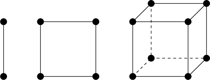
The -dimensional hypercube, denoted , has vertices, each labeled with a binary word with length . Two vertices are connected by an edge if their words differ in exactly one component (see Figure 6). This graph is isomorphic to the Cartesian product of copies of , the complete graph with two vertices. The Laplacian of is
whose two eigenvalues are and . The one-dimensional hypercube is just . Higher dimensional hypercubes are defined recursively:
By equation (12), their Laplacian matrices are
Using equation (13) recursively, the Laplacian of has eigenvalues , , each with multiplicity . The FMMC is achieved for:
This solution has also been worked out, for example, in [Moh97].
3.3 FMMC on distance-transitive graphs
Distance-transitive graphs have been studied extensively in the literature (see, e.g., [BCN89]). In particular, they are both edge- and vertex-transitive. In previous examples, the cycles and the hypercubes are actually distance-transitive graphs; so are the bipartite graphs when the two parties have equal number of vertices.
In a distance-transitive graph, all vertices have the same valency, which we denote by . The Laplacian matrix can be written as , with being the adjacency matrix. Therefore
We can substitute the above equation in equations (6) and (7) to obtain the optimal solution in terms of and .
Since distance-transitive graphs usually have very large automorphism groups, the eigenvalues of the adjacency matrix (and the Laplacian ) often have very high multiplicities. But to solve the FMMC problem, we only need to know the distinct eigenvalues; actually, only and would suffice. In this regard, it is more convenient to use a much smaller matrix, the intersection matrix, which has all the distinct eigenvalues of the adjacency matrix.
Let be the diameter of the graph. For a nonnegative integer , choose any two vertices and such that their distance satisfies . Let , and be the number of vertices that are adjacent to and whose distance from are , and , respectively. That is,
For distance-transitive graphs, these numbers are independent of the particular pair of vertices and chosen. Clearly, we have , and . The intersection matrix is the following tridiagonal matrix
Denote the eigenvalues of the intersection matrix, in decreasing order, as . These are precisely the distinct eigenvalues of the adjacency matrix (see, e.g., [Big74]). In particular, we have
The following corollary is a direct consequence of Theorem 3.1.
Corollary 3.2.
The optimal solution of the FMMC problem on a distance-transitive graph is
| (14) | |||||
| (15) |
Next we give solutions for the FMMC problem on several families of distance-transitive graphs.
3.3.1 Complete graphs
The case of the complete graph with vertices, usually called , is very simple. It is distance-transitive, with diameter and valency . The intersection matrix is
with eigenvalues , . Using equations (14) and (15), the optimal parameters are
The associated matrix has one eigenvalue equal to 1, and the remaining eigenvalues vanish. Such Markov chains achieve perfect mixing after just one step, regardless of the value of .
3.3.2 Petersen graph
The Petersen graph, shown in Figure 7, is a well-known distance-transitive graph with 10 vertices and 15 edges. The diameter of the graph is , and the intersection matrix is
with eigenvalues , and . Applying the formula (14) and (15), we obtain

3.3.3 Hamming graphs
The Hamming graphs, denoted , have vertices labeled by elements in the Cartesian product , with two vertices being adjacent if they differ in exactly one component. By the definition, it is clear that Hamming graphs are isomorphic to the Cartesian product of copies of the complete graph . Hamming graphs are distance-transitive, with diameter and valency . Their eigenvalues are given by for . These can be obtained using an equation for eigenvalues of adjacency matrices, similar to (13), with the eigenvalues of being and . Therefore the FMMC has parameters:
We note that hypercubes (see §3.2.2) are special Hamming graphs with .
3.3.4 Johnson graphs
The Johnson graph (for ) is defined as follows: the vertices are the -element subsets of , with two vertices being connected with an edge if and only if the subsets differ exactly by one element. It is a distance-transitive graph, with vertices and edges. It has valency and diameter . The eigenvalues of the intersection matrix can be computed analytically and they are:
Therefore, by Corollary 3.2, we obtain the optimal transition probability
and the smallest SLEM
4 FMMC on orbit graphs
For graphs with large automorphism groups, the eigenvalues of the transition probability matrix often have very high multiplicities. To solve the FMMC problem, it suffices to work with only the distinct eigenvalues without consideration of their multiplicities. This is exactly what the intersection matrix does for distance-transitive graphs. In this section we develop similar tools for more general graphs. More specifically, we show how to construct an orbit chain which is much smaller in size than the original Markov chain, but contains all its distinct eigenvalues (with much fewer multiplicities). The FMMC on the original graph can be found by solving a much smaller problem on the orbit chain.
4.1 Orbit theory
Here we review the orbit theory developed in [BDPX05]. Let be a symmetric Markov chain on the graph , and be a group of automorphisms of the graph. Often, it is a subgroup of the full automorphism group . The vertex set partitions into orbits . For notational convenience, in this section we use , for , to denote entries of the transition probability matrix. We define the orbit chain by specifying the transition probabilities between orbits
| (16) |
This transition probability is independent of which is chosen, so it is well defined and the lumped orbit chain is indeed Markov.
The orbit chain is in general no longer symmetric, but it is always reversible. Let , , be the stationary distribution of the original Markov chain. Then the stationary distribution on the orbit chain is obtained as
| (17) |
It can be verified that
| (18) |
which is the detailed balance condition to test reversibility.
The following is a summary of the orbit theory we developed in [BDPX05], which relate the eigenvalues and eigenvectors of the orbit chain to the eigenvalues and eigenvectors of the original chain .
- •
Lifting ([BDPX05, §3.1]). If is an eigenvalue of with associated eigenvector , then is an eigenvalue of with -invariant eigenfunction . Conversely, every -invariant eigenfunction appears uniquely from this construction.
- •
Projection ([BDPX05, §3.2]). Let be an eigenvalue of with eigenvector . Define . Then appears as an eigenvalue of , with eigenvector , if either of the following two conditions holds:
- (a)
has a fixed point and .
- (b)
is nonzero at a vertex in an -orbit which contains a fixed point of .
- (a)
Equipped with this orbit theory, we would like to construct one or multiple orbit chains that retain all the eigenvalues of the original chain. Ideally the orbit chains are much smaller in size than the original chain, with the eigenvalues having much fewer multiplicities. The following theorem (Theorem 3.7 in [BDPX05]) gives sufficient conditions that guarantee that the orbit chain(s) attain all the eigenvalues of the original chain.
Theorem 4.1.
Suppose that is a disjoint union of the orbits under . Let be the subgroup of that has a fixed point in . Then all eigenvalues of occur among the eigenvalues of . Further, every eigenvector of occurs by lifting an eigenvector of some .
Observe that if , then the eigenvalues of contain all eigenvalues of . This allows disregarding some of the in Theorem 4.1. In particular, it is possible to construct a single orbit chain that contains all eigenvalues of the original chain. Therefore we have
Corollary 4.2.
Suppose that is a disjoint union of the orbits under , and is a subgroup of . If has a fixed point in every , then all distinct eigenvalues of occur among the eigenvalues of .
Remarks.
To find in the above corollary, we can just compute the corresponding stabilizer, i.e., compute the largest subgroup of that fixes one point in each orbit. Note that the promised by the corollary may be trivial in some cases; see the example in §5.3.6.


We illustrate the orbit theory with the bipartite graph shown in Figure 4. It is easy to see that is the direct product of two symmetric groups, namely , with each symmetric group permuting one of the two subsets of vertices. This graph is edge-transitive. So we assign the same transition probability on all the edges.
The orbit chains under four different subgroups of are shown in Figure 8. The transition probabilities between orbits are calculated using equation (16). Since the transition probabilities are not symmetric, we represent the orbit chains by directed graphs, with different transition probabilities labeled on opposite directions between two adjacent vertices. The full automorphism group has two orbits of vertices; see Figure 8(a). The orbit graphs under the subgroups (Figure 8(b)) and (Figure 8(c)) each contains a fixed point of the two orbits under . By Theorem 4.1, these two orbit chains contain all the distinct eigenvalues of the original chain on . Alternatively, we can construct the orbit chain under the subgroup , shown in Figure 8(d). This orbit chain contain a fixed point in both orbits under . By Corollary 4.1, all distinct eigenvalues of appear in this orbit chain. In particular, this shows that there are at most four distinct eigenvalues in the original chain.
4.2 Fastest mixing reversible Markov chain on orbit graph
Since in general the orbit chain is no longer symmetric, we cannot directly use the convex optimization formulation (1) or (2) to minimize . Fortunately, the detailed balance condition (18) leads to a simple transformation that allow us to formulate the problem of finding the fastest reversible Markov chain as a convex program [BDX04].
Suppose the orbit chain contains all distinct eigenvalues of the original chain. Let be the stationary distribution of the orbits, and let . The detailed balance condition (18) can be written as , which implies that the matrix is symmetric (and of course, has the same eigenvalues as ). The eigenvector of associated with the maximum eigenvalue is . The SLEM equals the spectral norm of restricted to the orthogonal complement of the subspace spanned by . This can be written as
Introducing a scalar variable to bound the above spectral norm, we can formulate the fastest mixing reversible Markov chain problem as an SDP
| (19) |
The optimization variables are the matrix and scalar , and problem data is given by the orbit graph and the stationary distribution . Note that the reversibility constraint can be dropped since it is always satisfied by the construction of the orbit chain; see equation (18). By pre- and post-multiplying the matrix inequality by , we can write then another equivalent formulation:
| (20) |
To solve the fastest mixing reversible Markov chain problem on the orbit graph, we need the following three steps.
- 1.
Conduct symmetry analysis on the original graph: identify the automorphism graph and determine the number of orbits of edges . By Corollary 2.2, this is the number of transition probabilities we need to consider.
- 2.
Find a group of automorphisms that satisfies the conditions in Corollary 4.2. Construct its orbit chain by computing the transition probabilities using equation (16), and compute the stationary distribution using equation (17). Note that the entries of are multiples of the transition probabilities on the original graph.
- 3.
Solve the fastest mixing reversible Markov chain problem (19). The optimal SLEM is also the optimal SLEM for the original chain, and the optimal transition probabilities on the original chain can be obtained by simple scaling of the optimal orbit transition probabilities.
We have assumed a single orbit chain that contains all distinct eigenvalues of the original chain. Sometimes it is more convenient to use multiple orbit chains. Let , , be the collection of orbit chains in Theorem 4.1. In this case we need to minimize . This can be done by simply adding the set of constraints in (19) for every matrix . For example, for the complete bipartite graph , instead of using the single orbit chain in Figure 8(d), we can use the two orbit chains in Figure 8(b) and Figure 8(c) together, with two sets of constraints in the SDP (19).
4.3 Examples
We demonstrate the above computational procedure on orbit graphs with two examples: the graph - and the complete binary tree. Both examples will be revisited in §5 using the method of block diagonalization.
4.3.1 The graph -


The graph - consists of two copies of the complete graph joined by a bridge (see Figure 9(a)). We follow the three steps described in §4.2.
First, it is clear by inspection that the full automorphism group is . The actions of are all possible permutations of the two set of vertices, distinct from the two center vertices and , among themselves. The group acts on the graph by switching the two halves. The semi-direct product symbol means that the actions of and do not commute.
By symmetry analysis in §2, there are three edge orbits under the full automorphism group: the bridging edge between vertices and , the edges connecting and to all other vertices, and the edges connecting all other vertices. Thus it suffices to consider just three transition probabilities , , and , each labeled in Figure 9(a) on one representative of the three edge orbits.
As the second step, we construct the orbit chains. The orbit chain of - under the full automorphism group is depicted in Figure 9(b). The orbit includes vertices and , and the orbit consists of all other vertices. The transition probabilities of this orbit chain are calculated from equation (16) and are labeled on the directed edges in Figure 9(b). Similarly, the orbit chain under the subgroup is depicted in Figure 9(c). While these two orbit chains are the most obvious to construct, none of them contains all eigenvalues of the original chain, nor does their combination. For the one in Figure 9(b), the full automorphism group does not have a fixed point either of its orbit or . For the one in 9(c), the automorphism group has a fixed point in (either or ), but does not have a fixed point in (note here is the orbit of under the full automorphism group). To fix the problem, we consider the orbit chain under the group , which leave the vertex , , and fixed, while permuting the rest vertices on the left and the points on the right, respectively. The corresponding orbit chain is shown in Figure 9(d). By Corollary 4.2, all distinct eigenvalues of the original Markov chain on - appear as eigenvalues of this orbit chain. Thus there are at most five distinct eigenvalues in the original chain no matter how large is.
To finish the second step, we calculate the transition probabilities of the orbit chain under using equation (16) and label them in Figure 9(d). If we order the vertices of this orbit chain as , then the transition probability matrix on the orbit chain is
By equation (17), the stationary distribution of the orbit chain is
As the third step, we solve the SDP (19) with the above parametrization. It is remarkable to see that we only need to solve an SDP with variables (three transition probabilities , , , and the extra scalar ) and matrices no matter how large the graph (the number ) is.
We will revisit this example in §5.3.4 using the block diagonalization method, where we present an analytic expression for the exact optimal SLEM and corresponding transition probabilities.
4.3.2 Complete binary tree
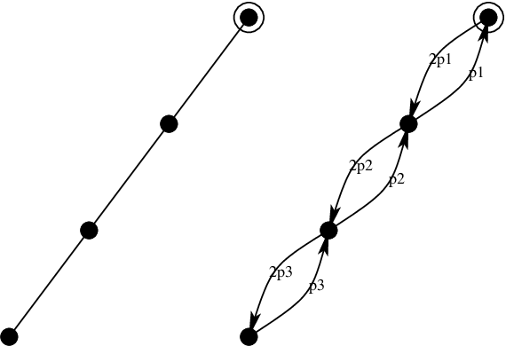
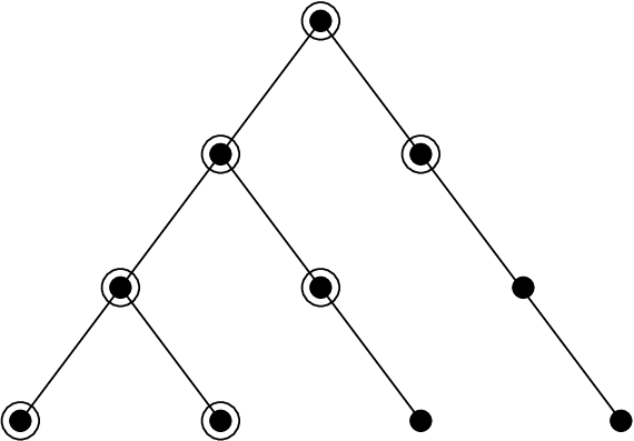
We consider a complete binary tree with levels of branches, denoted as . The total number of nodes is . The matrix inequalities in the corresponding SDP have size , which is clearly exponential in . However, the binary tree has a very large automorphism group, of size . This automorphism group is best described recursively. Plainly, for , we have . For , it can be obtained by the recursion
where represents the wreath product of two groups (e.g., [JK81]). More specifically, let and be elements of the product group , and and be in . The multiplication rule of the wreath product is
This is a semi-direct product (cf. the automorphism group of -). From the above recursion, the automorphism group of is
(The wreath product is associative, but not commutative.) The representation theory of the automorphism group of the binary tree has been thoroughly studied as this group is the Sylow 2-subgroup of a symmetric group; see [OOR04, AV05].
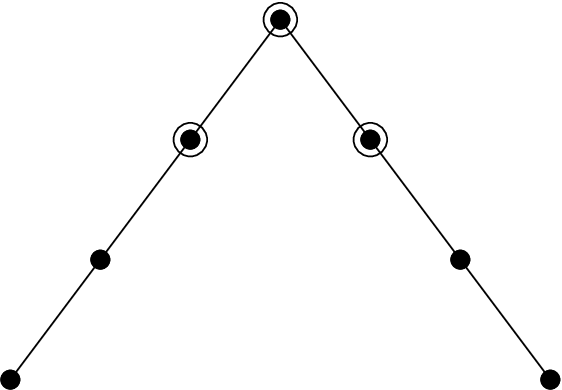
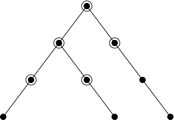
The orbit graph of under its full automorphism group is a path with nodes (Figure 10(a), left). Since there are orbits of edges, there are different transition probabilities we need to consider. We label them as , , from top to bottom of the tree. The corresponding orbit chain, represented by a directed graph labeled with transition probabilities between orbits, is shown on the right of Figure 10(a). To simplify presentation, only the orbit graphs are shown in other subfigures of Figure 10. The corresponding orbit chains should be straightforward to construct.
The largest subgroup of that has a fixed point in every orbit under is
where denotes direct product of groups. The corresponding orbit graph is shown in Figure 10(d) for . The number of vertices in this orbit graph is
which is much smaller than , the size of .
From the above analysis, we only need to solve the fastest reversible Markov chain problem on the orbit graph of size with variables . In next section, using the technique of block diagonalization, we will see that the transition probability matrix of size can be further decomposed into smaller matrices with sizes . Due to an eigenvalue interlacing result, we only need to consider the orbit chain with vertices in Figure 10(b).
5 Symmetry reduction by block diagonalization
By definition of the fixed-point subspace (in §2.2), any transition probability matrix is invariant under the actions of . More specifically, for any permutation matrix given by , we have , equivalently . In this section we show that this property allows the construction of a coordinate transformation matrix that can block diagonalize every . The resulting blocks usually have much smaller sizes and repeated blocks can be discarded in computation.
The method we use in this section is based on classical group representation theory (e.g., [Ser77]). It was developed for more general SDPs in [GP04], and has found applications in sum-of-squares decomposition for minimizing polynomial functions [Par00, Par03, PS03] and controller design for symmetric dynamical systems [CLP03]. A closely related approach is developed in [dKPS07], which is based on a low-order representation of the commutant (collection of invariant matrices) of the matrix algebra generated by the permutation matrices.
5.1 Some group representation theory
Let be a group. A representation of assigns an invertible matrix to each in such a way that the matrix assigned to the product of two elements in is the product of the matrices assigned to each element: . The matrices we work with are all invertible and are considered over the real or complex numbers. We thus regard as a homomorphism from to the linear maps on a vector space . The dimension of is the dimension of . Two representations are equivalent if they are related by a fixed similarity transformation.
If is a subspace of invariant under , then restricted to gives a subrepresentation. Of course the zero subspace and the subspace are trivial subrepresentations. If the representation admits no non-trivial subrepresentation, then is called irreducible.
We consider first complex representations, as the theory is considerably simpler in this case. For a finite group there are only finitely many inequivalent irreducible representations of dimensions , respectively. The degrees divide the group order , and satisfy the condition . Every linear representation of has a canonical decomposition as a direct sum of irreducible representations
where are the multiplicities. Accordingly, the representation space has an isotypic decomposition
| (21) |
where each isotypic components consists of invariant subspaces
| (22) |
each of which has dimension and transforms after the manner of . A basis of this decomposition transforming with respect to the matrices is called symmetry-adapted and can be computed using the algorithm presented in [Ser77, §2.6-2.7] or [FS92, §5.2]. This basis defines a change of coordinates by a matrix collecting the basis as columns. By Schur’s lemma, if a matrix satisfies
| (23) |
then has block diagonal form with one block for each isotypic component of dimension , which further decomposes into equal blocks of dimension . That is
| (24) |
For our application of semidefinite programs, the problems are presented in terms of real matrices, and therefore we would like to use real coordinate transformations. In fact a generalization of the classical theory to the real case is presented in [Ser77, §13.2]. If all are real matrices the irreducible representation is called absolutely irreducible. Otherwise, for each with complex character its complex conjugate will also appear in the canonical decomposition. Since is real both will have the same multiplicity and real bases of can be constructed. So two complex conjugate irreducible representations form one real irreducible representation of complex type. There is a third case, real irreducible representations of quaternonian type, rarely seen in practical examples.
In this paper, we assume that the representation is orthogonal, i.e., for all . As a result, the transformation matrix can also be chosen to be orthogonal. Thus (for complex matrices, it is the conjugate transpose). For symmetric matrices the block corresponding to a representation of complex type or quaternonian type simplifies to a collection of equal subblocks. For the special case of circulant matrices, complete diagonalization reveals all the eigenvalues [Dia88, page 50].
5.2 Block diagonalization of SDP constraint
As in §2.2, for every we assign a permutation matrix by letting if and otherwise. This is an -dimensional representation of , which is often called the natural representation. As mentioned in the beginning of this section, every matrix in the fixed-point subset has the symmetry of ; i.e., it satisfies the condition (23) with . Thus a coordinate transformation matrix can be constructed such that can be block diagonalized into the form (24).
Now we consider the SDP (5), which is the FMMC problem formulated in the fixed-point subset . In §2.3, we have derived the expression , where is the Laplacian matrix for the th orbit graph and is the common transition probability assigned on all edges in the th orbit graph. Note the matrix has the symmetry of . Applying the coordinate transformation to the linear matrix inequalities, we obtain the following equivalent problem
| (25) |
where correspond to the small blocks in (24) of the transformed matrix , and are the corresponding diagonal blocks of . The number of matrix inequalities is the number of inequivalent irreducible representations, and the size of each matrix inequality is the multiplicity of the corresponding irreducible representation. Note that we only need one out of copies of each in the decomposition (24). Since can be much smaller than (the number of vertices in the graph), the improvement in computational complexity over the SDP formulation (5) can be significant (see the flop counts discussed in §1.2). This is especially the case when there are high-dimensional irreducible representations (i.e., when is large; see, e.g., - defined in §4.3.1).
The transformed SDP formulation (25) needs some further justification. Namely, all the off-diagonal blocks of the matrix have to be zero. This is in fact the case. Moreover, the following theorem reveals an interesting connection between the block diagonalization approach and the orbit theory in §4.
Theorem 5.1.
Let be a subgroup of , and be the coordinate transformation matrix whose columns are a symmetry-adapted basis for the natural representation of . Suppose a Markov chain defined on the graph has the symmetry of . Then the matrix has the same block diagonal form as . Moreover, there is only one nonzero block. Without loss of generality, let this nonzero block be and the corresponding block of be . These two blocks relate to the orbit chain by
| (26) | |||||
| (27) |
where , , and is the stationary distribution of .
Proof.
First we note that always has a single eigenvalue with associated eigenvector . Thus spans an invariant subspace of the natural representation, which is obviously irreducible. The corresponding irreducible representation is isomorphic to the trivial representation (which assigns the scalar to every element in the group). Without loss of generality, let be the isotypic component that contains the vector . Thus is a direct product of -fixed vectors (each corresponds to a copy of the trivial representation), and is a linear combination of these vectors.
Let be the dimension of , which is the number of -fixed vectors. We can calculate by Frobenius reciprocity, or “Burnside’s Lemma”; see, e.g., [Ser77]. To do so, we note that the character of the natural representation , , is the number of fixed points of , i.e.,
“Burnside’s Lemma” says that
The left-hand side is the inner product of with the trivial representation. It thus counts the number of -fixed vectors in . So equals the number of orbits under .
Suppose that as a disjoint union of -orbits. Let if and zero otherwise. Then are -fixed vectors, and they form an orthonormal symmetry-adapted basis for (these are not unique). Let be the first columns of . They are orthogonal to all other columns of . Since is a linear combination of , it is also orthogonal to other columns of . Therefore the matrix has all its elements zero except for the first diagonal block, which we denote as . More specifically, where
Note that by (17) the stationary distribution of the orbit chain is
Thus we have . This proves (27).
Finally we consider the relationship between and . We prove (26) by showing
It is straightforward to verify that
The entry at the -th row and -th column of the matrix are given by
In the last equation, we have used the fact that is independent of which is chosen. This completes the proof. ∎
From Theorem 5.1, we know that contains the eigenvalues of the orbit chain under . Other blocks contain additional eigenvalues (not including those of ) of the orbit chains under various subgroups of . (Note that the eigenvalues of the orbit chain under are always contained in the orbit chain under its subgroups). With this observation, it is possible to identify the multiplicities of eigenvalues in orbit chains under various subgroups of by relating to the decompositions (21), (22) and (24) (some preliminary results are discussed in [BDPX05]).
5.2.1 A running example

As a running example for this section, we consider a Markov chain on a grid , with a total of 9 nodes (see Figure 11). The automorphism group is isomorphic to the 8-element dihedral group , and corresponds to flips and 90-degree rotations of the graph. The orbits of acting on the vertices and edges are
and
respectively. So is neither vertex- nor edge-transitive.
By Corollary 2.2, we associate transition probabilities and to the two edge orbits, respectively. The transition probability matrix has the form
The matrix satisfies for every . Using the algorithm in [FS92, §5.2], we found a symmetry-adapted basis for the representation , which we take as columns to form
With this coordinate transformation matrix, we obtain
The 3-dimensional block contains the single eigenvalue , and it is related to the orbit chain in Figure 12 by the equation (26). The corresponding nonzero block of is

Next, we substitute the above expressions into the SDP (25) and solve it numerically. Since there are repeated blocks, the original matrix is replaced by four smaller blocks, of dimension 3,1,1,2. The optimal solutions are
Interestingly, it can be shown that these optimal values are not rational, but instead algebraic numbers with defining minimal polynomials:
5.3 Examples
We revisit some previous examples with the block diagonalization method, and draw connections to the method based on orbit theory in §4. We also discuss some additional examples that are difficult if one uses the orbit theory, but are nicely handled by block diagonalization. In many of the examples, the coordinate transformation matrix can be constructed directly by inspection.
5.3.1 Complete bipartite graphs
For the complete bipartite graph (see Figure 4), This graph is edge-transitive, so we can assign the same transition probability on all the edges. The transition probability matrix has the form
We can easily find a decomposition of the associated matrix algebra. It will have three blocks, and an orthogonal block-diagonalizing change of basis is given by
where is an matrix whose columns are an orthogonal basis of the subspace complementary to that generated by .
In the new coordinates, the matrix has the following diagonal blocks
The block has eigenvalues and . The other diagonals reveal the eigenvalue and , with multiplicities and , respectively. The optimal solution to the FMMC problem can be easily obtained as in (10) and (11).
To draw connections to the orbit theory, we note that the above block is precisely in the equation (26), and the corresponding is the orbit chain shown in Figure 8(a). In addition to the two eigenvalues in , the extra eigenvalue in the orbit chain of Figure 8(b) is , and the extra eigenvalue in Figure 8(c) is . All these eigenvalues appear in the orbit chain in Figure 8(d). As we have seen, the block diagonalization technique reveals the multiplicities in the original chain of the eigenvalues from various orbit chains.
5.3.2 Complete -partite graphs
The previous example generalizes nicely to the complete -partite graph . In this case, the fixed-point reduced matrix will have dimensions , and the structure
where the probabilities satisfy . There are total independent variables.
In a very similar fashion to the bipartite case, we can explicitly write the orthogonal coordinate transformation matrix
The matrix decomposes into blocks: one of dimension , with the remaining blocks each having dimension . The decomposition is:
These blocks can be substituted into the SDP (25) to solve the FMMC problem.
5.3.3 Wheel graph

The wheel graph consists of a center vertex (the hub) and a ring of peripheral vertices, each connected to the hub; see Figure 13. It has total nodes. Its automorphism group is isomorphic to the dihedral group with order . The transition probability matrix has the structure
| (31) |
where and are the transition probabilities between the hub and each peripheral vertex, and between adjacent peripheral vertices, respectively.
For this structure, the block-diagonalizing transformation is given by
where is the unitary Fourier matrix of size . As a consequence, the matrix is block diagonal with a matrix and scalars on its diagonal, given by
and
where is an elementary -th root of unity. The block is , which contains eigenvalues of the orbit chain under (it has only two orbits).
With the above decomposition, we obtain the optimal solution to the FMMC problem in closed form
The optimal value of the SLEM is
Compared with the optimal solution for the cycle graph in (8) and (9), we see an extra factor of in both the SLEM and the transition probability between peripheral vertices. This is exactly the factor improved by adding the central hub over the pure -cycle case.
The wheel graph is an example for which the block diagonalization technique works out nicely, while the orbit theory leads to much less reduction. Although there are only two orbits under the full automorphism group, any orbit graph that has a fixed peripheral vertex will have at least orbits (the corresponding symmetry is the reflection through that vertex).
5.3.4 -
We did careful symmetry analysis for the graph - in §4.3.1; see Figure 9. The transition probability matrix on this graph has the structure
where is a circulant matrix
Since circulant matrices are diagonalized by Fourier matrices, we first use the transformation matrix
where is the unitary Fourier matrix of dimension . This corresponds to block diagonalization using the symmetry group , which is a subgroup of . The matrix has diagonal blocks
and
| (32) |
From this we know that has an eigenvalue with multiplicity , and the remaining four eigenvalues are the eigenvalues of the above block . The block corresponds to the orbit chain under the symmetry group . More precisely, , where , and are the transition probability matrix and stationary distribution of the orbit chain shown in Figure 9(c), respectively.
Exploring the full automorphism group of -, we can further block diagonalize . Let
The block is decomposed into
The first block is , which has eigenvalues and . By Theorem 5.1, is related to the orbit chain under (see Figure 9(b)) by the equation (26). The second block has eigenvalues
These are the eigenvalues contained in the orbit chain of Figure 9(c) but not in Figure 9(b).
In summary, the distinct eigenvalues of the Markov chain on - are
where the last one has multiplicity , and all the rest have multiplicity 1. To solve the FMMC problem, we still need to solve the SDP (25). There are three blocks of matrix inequality constraints, with sizes , , , respectively. Note that the total size is , which is exactly the size of the single matrix inequality in the SDP (19) when we used the orbit theory to do symmetry reduction. As we mentioned before, the huge reduction for - is due to the fact that it has an irreducible representation with high dimension and multiplicity (see [BDPX05, Proposition 2.4]). In the decomposition (24), this means a block of size repeated times; see equation (32).
Since now the problem has been reduced to something much more tractable, we can even obtain an analytic expression for the optimal transition probabilities. The optimal solution for the - graph (for ) is given by:
The corresponding optimal convergence rate is
For large , we have . This is quite close to the SLEM of a suboptimal construction with transition probabilities
| (33) |
As shown in [BDPX05], the corresponding SLEM is of the order ; here we have . The limiting value of the optimal transition probability between the two clusters is .
5.3.5 Complete binary trees
Since the automorphism groups of the complete binary trees are given recursively (see §4.3.2), it is also convenient to write the transition probability matrices in a recursive form. We start from the bottom by considering the last level of branches. If we cut-off the rest of the tree, the last level has three nodes and two edges with the transition probability matrix
| (34) |
For the tree with levels , the transition matrix can be computed from the recursion
| (35) |
where , a unit vector in with .
The coordinate transformations are also best written in recursive form. Let
and define the matrices
It is clear that all the are orthogonal. It is easy to verify that block-diagonalizes
In fact block-diagonalizes , and the transformed matrices can be obtained recursively
for .
The matrix has a very special structure. It has distinct blocks, each with size , respectively. Order these blocks with increasing sizes as . The largest block of size is
The matrix is the submatrix of by removing its first row and column. The matrix is the submatrix of by removing its first two rows and first two columns, and so on. The matrix is just the scalar . The matrix only appears once and it is related by (26) to the orbit chain in Figure 10(a) (for this example we use instead of for notational convenience). The eigenvalues of appear in with multiplicity one. For , the block is repeated times. These blocks, in a recursive form, contain additional eigenvalues of , and the numbers of their occurrences reveal the multiplicities of the eigenvalues.
More specifically, we note that the orbit chain under the full automorphism group has only one fixed point — the root vertex (see Figure 10(a)). We consider next the orbit chain that has a fixed point in the first level of child vertices (the other child vertex in the same level is also fixed). This is the orbit graph in Figure 10(b), which has vertices. The matrix contains exactly the eigenvalues that appear in this orbit chain but not in the one of Figure 10(a). These eigenvalues each has multiplicity in . Then we consider the orbit chain that has a fixed point in the second level of child vertices (it also must have a fixed point in the previous level). This is the orbit graph in Figure 10(c), which has vertices. The matrix contains exactly the eigenvalues that appear in this orbit chain but not in the previous one. These eigenvalues each has multiplicity . In general, for , the size of the orbit chain that has a fixed point in the -th level of child vertices is
(it must have a fixed point in all previous levels). Compared with the orbit chain of -th level, the orbit chain of -th level contains additional eigenvalues. These are precisely the eigenvalues of the matrix , and they all appear in with multiplicity .
Because of the special structure of , we have the following eigenvalue interlacing result (e.g., [HJ85, Theorem 4.3.8])
for . Thus for the FMMC problem, we only need to consider the two blocks and (note that ). In other words, we only need to consider the orbit chain with vertices in Figure 10(b). This is a further simplification over the method based on orbit theory.
We conjecture that the optimal transition probabilities are
Notice that these probabilities do not depend explicitly on , and so they coincide for any two binary trees, regardless of the height. With increasing , the limiting optimal values oscillate around and converge to .
5.3.6 An example of Ron Graham


We finish this section with an example raised by Ron Graham. Consider the simplest graph with no symmetry (Figure 14, left). Take copies of this six vertex graph and join them, head to tail, in a cycle. By construction, this vertex graph certainly has symmetry. Careful examination reveals that the automorphism group is isomorphic to the dihedral group (with order ). The construction actually brings symmetry under reflections in addition to rotations (Figure 14, right). The orbit graphs under and are shown in Figure 15.
Although the automorphism group of this graph (with vertices) is isomorphic to the ones of -cycles (Figure 3) and wheels (Figure 13), finding the symmetry-adapted basis for block-diagonalization is a bit more involved. This is due to the different types of orbits we have for this graph. The details of block-diagonalizing this type of graphs is described in [FS92, §3.1]. The diagonal blocks of the resulting matrix all have sizes no larger than . Numerical experiments show that for , the fastest mixing chain seems to satisfy
Intuitively, this vertex graph is the same as modifying a vertex cycle by adding a triangular bump (with an additional vertex) for every vertices. Recall that for a pure cycle, we have to use a transition probability that is slightly less than to achieve fastest mixing; see equation (8). Here because of the added bumps, it seems optimal to assign transition probability to every edge on the cycle ( and ), except for edges being part of a bump. For the bumps, the probability is shared between the original edge on the cycle () and the edge connecting to the bump points (). Moreover, we observe that as increases, gets smaller and gets closer to . So for large , the added bump vertices seem to be ignored, with very small probability to be reached; but once it is reached, it will staying there with high probability.
6 Conclusions
We have shown that exploiting graph symmetry can lead to significant reduction in both the number of variables and the size of matrices, in solving the FMMC problem. For special classes of graphs such as edge-transitive and distance-transitive graphs, symmetry reduction leads to closed form solutions in terms of the eigenvalues of the Laplacian matrix or the intersection matrix. For more general graphs, we gave two symmetry reduction methods, based on orbit theory and block diagonalization, respectively.
The method based on orbit theory is very intuitive, but the construction of “good” orbit chains can be of more art than technique. The method of block diagonalization can be mostly automated once the irreducible representations of the automorphism groups are generated (for small graphs, they can be generated using software for computational discrete algebra such as GAP [gro05]). These two approaches have an interesting connection: orbit theory gives nice interpretation of the diagonal blocks, while the block diagonalization approach offers theoretical insights about the construction of the orbit chains.
The symmetry reduction method developed in this paper can be very useful in many combinatorial optimization problems where the graph has rich symmetry properties, in particular, problems that can be formulated as or approximated by SDP or eigenvalue optimization problems involving weighted Laplacian matrices (e.g., [MP93, Goe97]). In addition to the reduction of problem size, other advantages of symmetry exploitation includes degeneracy removal, better conditioning and reliability [GP04].
There is still much to do in understanding how to exploit symmetry in semidefinite programming. The techniques presented in this paper requires a good understanding of orbit theory, group representation theory and interior-point methods for SDP. It is of practical importance to develop general purpose methods that can automatically detect symmetries (e.g., the code nauty [McK03] for graph automorphisms), and then exploit them in computations. A good model here is general purpose (but heuristic) methods for exploiting sparsity in numerical linear algebra, where symbolic operations on graphs (e.g., minimum degree permutation) reduce fill-ins in numerical factorization (e.g., [GL81]). As a result of this work, even very large sparse optimization problems are now routinely solved by users who are not experts in sparse matrix methods. For exploiting symmetry in SDP, the challenges include the development of fast methods to detect large symmetry groups (for computational purposes, it often suffices to recognize parts of the symmetries), and the integration of algebraic methods (e.g., orbit theory and group representations) and numerical algorithms (e.g., interior-point methods).
References
- [AV05] M. Abért and B. Virág. Dimension and randomness in groups acting on rooted trees. Journal of the American Mathematical Society, 18(1):157–192, 2005.
- [BCN89] A. E. Brouwer, A. M. Cohen, and A. Neumaier. Distance-Regular Graphs. Springer-Verlag, Berlin, 1989.
- [BDPX05] S. Boyd, P. Diaconis, P. A. Parrilo, and L. Xiao. Symmetry analysis of reversible Markov chains. Internet Mathematics, 2(1):31–71, 2005.
- [BDSX06] S. Boyd, P. Diaconis, J. Sun, and L. Xiao. Fastest mixing Markov chain on a path. The American Mathematical Monthly, 113(1):70–74, January 2006.
- [BDX04] S. Boyd, P. Diaconis, and L. Xiao. Fastest mixing Markov chain on a graph. SIAM Review, 46(4):667–689, 2004.
- [Big74] N. Biggs. Algebraic Graph Theory. Cambridge University Press, 1974.
- [BM03] S. Burer and R. D. C. Monteiro. A nonlinear programming algorithm for solving semidefinite programs via low-rank factorization. Mathematical Programming, Series B, 95:329–357, 2003.
- [Bré99] P. Brémaud. Markov Chains, Gibbs Fields, Monte Carlo Simulation and Queues. Texts in Applied Mathematics. Springer-Verlag, Berlin-Heidelberg, 1999.
- [BTN01] A. Ben-Tal and A. Nemirovski. Lectures on Modern Convex Optimization, Analysis, Algorithms, and Engineering Applications. MPS/SIAM Series on Optimization. SIAM, 2001.
- [BV04]
S. Boyd and L. Vandenberghe.
Convex Optimization.
Cambridge University Press, 2004.
Available at
http://www.stanford.edu/~boyd/cvxbook.html. - [BYZ00] S. Benson, Y. Ye, and X. Zhang. Solving large-scale sparse semidefinite programs for combinatorial optimization. SIAM Journal Optimization, 10:443–461, 2000.
- [Chu97] F. R. K. Chung. Spectral Graph Theory. Number 92 in CBMS Regional Conference Series in Mathematics. American Mathematical Society, 1997.
- [CLP03] R. Cogill, S. Lall, and P. A. Parrilo. On structured semidefinite programs for the control of symmetric systems. In Proceedings of 41st Allerton Conference on Communication, Control, and Computing, pages 1536–1545, Monticello, IL, October 2003.
- [DCS80] M. Doob, D. Cvetkovic, and H. Sachs. Spectra of Graphs: Theory and Application. Academic Press, New York, 1980.
- [Dia88] P. Diaconis. Group Representations in Probability and Statistics. IMS, Hayward, CA, 1988.
- [dKPS07] E. de Klerk, D. V. Pasechnik, and A. Schrijver. Reduction of symmetric semidefinite programs using the regular -representation. Mathematical Programming, Series B, 109:613–624, 2007.
- [DR07] I. Dukanovic and F. Rendl. Semidefinite programming relaxations for graph coloring and maximal clique problems. Mathematical Programming, Series B, 109:345–365, 2007.
- [DS91] P. Diaconis and D. Stroock. Geometric bounds for eigenvalues of Markov chains. The Annals of Applied Probability, 1(1):36–61, 1991.
- [DSC93] P. Diaconis and L. Saloff-Coste. Comparison theorems for reversible Markov chains. Ann. Appl. Probab., 3:696–730, 1993.
- [DSC06] P. Diaconis and L. Saloff-Coste. Separation cut-offs for birth and death chains. Submitted to Annals of Applied Probabilities, 2006.
- [ER63] P. Erdős and Rényi. Asymmetric graphs. Acta Math. Acad. Sci. Hungar., 14:295–315, 1963.
- [FS92] A. Fässler and E. Stiefel. Group Theoretical Methods and Their Applications. Birkhäuser, Boston, 1992.
- [Gat00] K. Gatermann. Computer Algebra Methods for Equivariant Dynamical Systems, volume 1728 of Lecture Notes in Mathematics. Springer-Verlag, 2000.
- [GL81] A. George and J. Liu. Computer Solution of Large Sparse Positive Definite Systems. Prentice Hall, Englewood Cliffs, NJ, 1981.
- [GL96] G. H. Golub and C. F. Van Loan. Matrix Computations. The John Hopkins University Press, Baltimore, 3rd edition, 1996.
- [GO06] K. K. Gade and M. L. Overton. Optimizing the asymptotic convergence rate of the Diaconis-Holmes-Neal sampler. To appear in Advances in Applied Mathematics, 2006.
- [Goe97] M. X. Goemans. Semidefinite programming in combinatorial optimization. Mathematical Programming, 79:143–161, 1997.
- [GP04] K. Gatermann and P. A. Parrilo. Symmetry groups, semidefinite programs, and sums of squares. Journal of Pure and Appl. Algebra, 192:95–128, 2004.
- [GR01] C. Godsil and G. Royle. Algebraic Graph Theory, volume 207 of Graduate Texts in Mathematics. Springer, 2001.
- [Gra81] A. Graham. Kronecker Products and Matrix Calculus with Applications. Ellis Horwoods Ltd., Chichester, UK, 1981.
- [gro05] The GAP group. GAP - groups, algorithms, programming - a system for computational discrete algebra, version 4.4.6, 2005. http://www.gap-system.org.
- [GSS88] M. Golubitsky, I. Stewart, and D. G. Schaeffer. Singularities and Groups in Bifurcation Theory II, volume 69 of Applied Mathematical Sciences. Springer, New York, 1988.
- [HJ85] R. A. Horn and C. A. Johnson. Matrix Analysis. Cambridge University Press, 1985.
- [HOY03] B. Han, M. L. Overton, and T. P.-Y. Yu. Design of Hermite subdivision schemes aided by spectral radius optimization. SIAM Journal on Matrix Analysis and Applications, 25:80–104, 2003.
- [HR00] C. Helmberg and F. Rendl. A spectral bundle method for semidefinite programming. SIAM Journal on Optimization, 10(3):673–696, 2000.
- [JK81] G. D. James and A. Kerber. The Representation Theory of the Symmetric Group. Addison-Wesley, Reading, Massachusetts, 1981.
- [KOMK01] Y. Kanno, M. Ohsaki, K. Murota, and N. Katoh. Group symmetry in interior-point methods for semidefinite programming. Optimization and Engineering, 2:293–320, 2001.
- [Lau07] M. Laurent. Strengthend semidefinite programming bounds for codes. Mathematical Programming, Series B, 109:239–261, 2007.
- [LNM04] Z. Lu, A. Nemirovski, and R. D. C. Monteiro. Large-scale semidefinite programming via saddle point mirror-prox algorithm. Submitted to Mathematical Programming, 2004.
- [Mar03] F. Margot. Exploiting orbits in symmetric ILP. Mathematical Programming, Series B, 98:3–21, 2003.
- [McK03] B.D. McKay. nauty User’s guide (Version 2.2). Australian National University, 2003. Available from http://cs.anu.edu.au/˜bdm/nauty/.
- [Mer94] R. Merris. Laplacian matrices of graphs: a survey. Linear Algebra and Its Applications, 197:143–176, 1994.
- [Moh97] B. Mohar. Some applications of Laplace eigenvalues of graphs. In G. Hahn and G. Sabidussi, editors, Graph Symmetry: Algebraic Methods and Applications, NATO ASI Ser. C 497, pages 225–275. Kluwer, 1997.
- [MP93] B. Mohar and S. Poljak. Eigenvalues in combinatorial optimization. In R. A. Brualdi, S. Friedland, and V. Klee, editors, Combinatorial and Graph-Theoretical Problems in Linear Algebra, volume 50 of IMA Volumes in Mathematics and Its Applications, pages 107–151. Springer-Verlag, 1993.
- [MR99] J. E. Marsden and T. Ratiu. Introduction to Mechanics and Symmetry, volume 17 of Texts in Applied Mathematics. Springer-Verlag, 2nd edition, 1999.
- [Nem04] A. Nemirovski. Prox-method with rate of convergence for variational inequalities with Lipschitz continuous monotone operators and smooth convex-concave saddle point problems. SIAM Journal on Optimization, 15(1):229–251, 2004.
- [Nes05] Y. Nesterov. Smooth minimization of non-smooth functions. Mathematical Programming, 103:127–152, 2005.
- [NN94] Y. Nesterov and A. Nemirovskii. Interior-Point Polynomial Algorithms in Convex Programming. SIAM Studies in Applied Mathematics. SIAM, 1994.
- [OOR04] R. C. Orellana, M. E. Orrison, and D. N. Rockmore. Rooted trees and iterated weath products of cyclic groups. Advances in Applied Mathematics, 33(3):531–547, 2004.
- [Ove92] M. L. Overton. Large-scale optimization of eigenvalues. SIAM Journal on Optimization, 2:88–120, 1992.
- [Par00] P. A. Parrilo. Structured semidefinite programs and semialgebraic geometry methods in robustness and optimization. PhD thesis, California Institute of Technology, May 2000. Available at http://resolver.caltech.edu/CaltechETD:etd-05062004-055516.
- [Par03] P. A. Parrilo. Semidefinite programming relaxations for semialgebraic problems. Mathematical Programming, 96:293 – 320, 2003.
- [PS03] P. A. Parrilo and B. Sturmfels. Minimizing polynomial functions. In S. Basu and L. Gonzalez-Vega, editors, Algorithmic and quantitative real algebraic geometry, volume 60 of DIMACS Series in Discrete Mathematics and Theoretical Computer Science, pages 83–99. AMS, 2003.
- [Roc05] S. Roch. Bounding fastest mixing. Electronic Communications in Probability, 10:282–296, 2005.
- [Saa92] Y. Saad. Numerical Methods for Large Eigenvalue Problems. Manchester University Press, Manchester, UK, 1992.
- [Sal06] J. Saltzman. A generalization of spectral analysis for discrete data using Markov chains. PhD thesis, Department of Statistics, Stanford University, 2006.
- [Ser77] J.-P. Serre. Linear Representations of Finite Groups. Springer-Verlag, New York, 1977.
- [Stu99] J. F. Sturm. Using SeDuMi 1.02, a MATLAB toolbox for optimization over symmetric cones. Optimization Methods and Software, 11-12:625–653, 1999. Special issue on Interior Point Methods (CD supplement with software).
- [TTT99] K. C. Toh, M. J. Todd, and R. H. Tutuncu. SDPT3 — a Matlab software package for semidefinite programming. Optimization Methods and Software, 11:545–581, 1999.
- [VB96] L. Vandenberghe and S. Boyd. Semidefinite programming. SIAM Review, 38(1):49–95, 1996.
- [Wor94] P. Worfolk. Zeros of equivariant vector fields: Algorithms for an invariant approach. Journal of Symbolic Computation, 17:487–511, 1994.
- [WSV00] H. Wolkowicz, R. Saigal, and L. Vandenberghe, editors. Handbook of Semidefinite Programming, Theory, Algorithms, and Applications. Kluwer Academic Publishers, 2000.
- [XB04] L. Xiao and S. Boyd. Fast linear iterations for distributed averaging. Systems and Control Letters, 53:65–78, 2004.
- [XBK07] L. Xiao, S. Boyd, and S.-J. Kim. Distributed average consensus with least-mean-square deviation. Journal of Parallel and Distributed Computing, 67:33–46, 2007.
- [YFK03] M. Yamashita, K. Fujisawa, and M. Kojima. Implementation and evaluation of SDPA 6.0 (semidefinite programming algorithm 6.0). Optimization Methods and Software, 18:491–505, 2003.