MCTP-07-28
CERN-PH-TH/2007-151
Cosmic Strings from Supersymmetric Flat Directions
Yanou Cuia, Stephen P. Martinb, David E. Morrisseya,
James D. Wellsc,a
a Michigan Center for Theoretical Physics (MCTP)
Physics Department, University of Michigan, Ann Arbor, MI 48109
b Physics Department, Northern Illinois University, DeKalb, IL 60115
Fermilab National Accelerator Laboratory, PO Box 500, Batavia IL 60510
c CERN, Theory Division, CH-1211 Geneva 23, Switzerland
August 11, 2026
Flat directions are a generic feature of the scalar potential in supersymmetric gauge field theories. They can arise, for example, from -terms associated with an extra abelian gauge symmetry. Even when supersymmetry is broken softly, there often remain directions in the scalar field space along which the potential is almost flat. Upon breaking a gauge symmetry along one of these almost flat directions, cosmic strings may form. Relative to the standard cosmic string picture based on the abelian Higgs model, these flat-direction cosmic strings have the extreme Type-I properties of a thin gauge core surrounded by a much wider scalar field profile. We perform a comprehensive study of the microscopic, macroscopic, and observational characteristics of this class of strings. We find many differences from the standard string scenario, including stable higher winding mode strings, the dynamical formation of higher mode strings from lower ones, and a resultant multi-tension scaling string network in the early universe. These strings are only moderately constrained by current observations, and their gravitational wave signatures may be detectable at future gravity wave detectors. Furthermore, there is the interesting but speculative prospect that the decays of cosmic string loops in the early universe could be a source of ultra-high energy cosmic rays or non-thermal dark matter. We also compare the observational signatures of flat-direction cosmic strings with those of ordinary cosmic strings as well as cosmic strings motivated by superstring theory.
1 Introduction
Cosmic strings are one-dimensional topological defects that can be formed in the early universe [1, 2, 3]. They are created if there is a phase transition in which a subgroup of a continuous symmetry is broken. Cosmic strings are stable because they carry a conserved topological charge. This charge is integer-valued, corresponding to , and is related to the number of times the phase of the breaking field winds at spatial infinity [4].
Unlike other types of topological defects, such as monopoles and domain walls, cosmic strings can be formed at a wide range of energy scales after inflation without severely contradicting the observed cosmology. The generic problem with topological defects is that, on account of their stability, they can easily come to dominate the energy density of the universe [3]. For cosmic strings there is an important loophole. Topological stability only applies to infinitely long strings. Cosmic string loops do not carry a net topological charge, and they can decay into particle or gravitational radiation. Such loops are formed when string segments intersect and exchange ends, or reconnect (or sometimes called intercommute). This allows a network of long cosmic strings to regulate its energy by chopping itself up into loops which radiate away. Indeed, for a wide range of initial string densities, analytic and numerical studies find that the competing processes of string stretching (from the cosmic expansion) and loop formation come to balance each other out. The network evolves towards a universal scaling solution whose properties are almost fully characterized by the cosmic string tension [5, 6, 7, 8, 9], independent of the initial conditions.
The vast majority of work on cosmic strings has focused on the abelian Higgs model, in which a gauge symmetry is spontaneously broken by the condensation of a charged scalar field. In this model, the vacuum expectation value (VEV) of the complex scalar field determines the mass of the gauge field, , and the physical scalar Higgs field, , through the relations
| (1.1) |
where is the gauge coupling, is the scalar quartic self-coupling, and is the VEV of the scalar. The relative size of and determines how the strings interact. For , parallel strings tend to repel at large distances while anti-parallel strings attract [3]. These strings are said to be Type-II, in analogy with superconductors. When , the strings attract for any relative orientation, and they are said to be Type-I. The attractive force between parallel Type-I strings allows them to form stable higher-winding modes.
In most field theories, including the abelian Higgs model, the masses and are naturally of the same order. Much of the previous work on cosmic strings has therefore dealt with Type-II or weakly Type-I strings. In the present work, we will instead investigate the behavior of very strongly Type-I cosmic strings, corresponding to . Our motivation to consider the extreme Type-I limit comes from supersymmetry [10]. As we will show below, there exist supersymmetric field theories in which arises in a natural way when a gauge symmetry is broken along a flat-direction of the scalar potential. Supersymmetry is essential because it ensures that quantum corrections do not lift the flat direction.
The key ingredients in our construction, supersymmetry and a new gauge symmetry, are each well-motivated in their own right independently of cosmic strings. Low-energy supersymmetry is one of the most elegant ways to explain the large hierarchy between the electroweak scale and the Planck scale [10]. It can also provide a candidate for the dark matter (DM) in the lightest superpartner particle (LSP), and in its minimal form, leads to an excellent unification of gauge couplings. Supersymmetry also plays an important role in superstring theories of gravity. Additional local symmetries arise in many models of new physics such as grand unified models and -brane constructions [11]. In supersymmetric models, such symmetries can also help to solve the problem [12].
A common feature of supersymmetric theories is the existence of directions in the scalar potential that are almost flat. To be precise, an almost flat direction is one for which the curvature of the potential near the minimum is much smaller than the scale of the (symmetry-breaking) VEV at that minimum. Typically, these directions in field space are completely flat at tree-level, when only renormalizable operators are included in the potential, but they are lifted by higher-dimensional operators, quantum effects, and supersymmetry breaking. As long as the supersymmetry breaking effects are both soft and small, the residual approximate supersymmetry prevents quantum corrections from destroying the flatness of the potential. When a gauge symmetry is broken along an almost-flat direction, the scalar excitation around the VEV along the flat direction is much lighter than the corresponding massive gauge boson. We will show that the cosmic strings associated with this pattern of gauge symmetry breaking are of the strongly Type-I sort [13, 14, 15, 16, 17, 19, 20].11 1 Let us also emphasize that the cosmic strings arising in general (approximately) supersymmetric theories need not be associated with a flat direction, and can also be of the Type-II variety. For examples, see Refs. [21, 22, 23, 24].
The interactions and cosmological consequences of strongly Type-I strings can be qualitatively different from those of Type-II and weakly Type-I strings [25, 26, 27]. When Type-I or Type-II cosmic strings intersect, they can reconnect or pass through each other. There is a third possible outcome when a pair of strongly Type-I strings intersect. Due to their mutual attraction, two strong Type-I strings with topological charges and can combine to form a single stable string with topological charge or . At the point of intersection, the incident strings can coalesce into a single higher-winding string, which may then proceed to grow like a zipper [26]. If this growth continues indefinitely, the outcome will be a single higher-winding mode string of horizon length. For Type-II and weakly Type-I strings, previous calculations and simulations predict that the outcome of a string intersection is reconnection with a probability close to unity, [28, 29, 30, 31]. Since reconnection is essential to the formation of string loops, which in turn are essential for the strings to be cosmologically viable, deviations away from can significantly alter the picture of cosmic strings in the early universe. In particular, if string zippering is common, there can exist a stable population of higher winding mode strings as well [32, 33, 34, 35].
Many of the exotic properties exhibited by the strongly Type-I cosmic strings arising from supersymmetric flat directions are also found in the cosmic strings emerging from superstring theory [36, 37, 38, 39, 40, 41, 42, 43], consisting of fundamental -strings and -strings. These cosmic superstrings can merge to form the equivalent of higher winding modes. In many cases they also have reconnection probabilities much less than unity, . However, flat-direction strings differ greatly from these strings in their microscopic properties. This is borne out in the the relationship between the (effective) topological charge and the string tension, as well as in the selection rules for string zippering. It may therefore be possible to distinguish strings from flat-direction strings with the observation of several string lensing events, each with a different apparent relative value for the string tension.
In the present work we study the properties and implications of cosmic strings derived from the breakdown of a gauge symmetry along a supersymmetric flat direction. We begin in Section 2 by studying the internal structure of flat-direction strings. Here, we present a simple toy model for the flat direction breaking, and we investigate approximate solutions to the equations of motion and study the string tensions using variational methods. In Section 3 we discuss the interactions between cosmic strings. We apply these results in Section 4, where we study the formation and evolution of flat-direction string networks in the early universe. The observational signatures produced by these networks will be the subject of Section 5. Finally, Section 6 is reserved for our conclusions.
Several earlier papers have investigated cosmic strings associated with flat-directions [13, 14, 15, 16, 17, 19, 20]. These studies have predominantly focused on the lowest () winding mode. We expand on these studies by exhibiting an explicit and natural field theory model for the strings, and by discussing the new features that arise from the existence of stable higher () winding modes. These modes significantly alter the cosmological picture of the strings.
2 String Profiles and Tensions
To begin, we introduce a simple class of models for a supersymmetric flat direction that could arise if there exists a gauge group in addition to those contained in the minimal supersymmetric standard model (MSSM). Within these models, we study the cosmic string solutions they support. In particular, we find approximate solutions to the classical equations of motion subject to the boundary conditions appropriate to a cosmic string, and we use these solutions to motivate a variational estimate of the string tension. Even though we focus on a particular class of models in the present section, we expect that many of the qualitative features that we find are also applicable to other cosmic string solutions associated with flat directions.
2.1 Flat Directions
As a prototypical model for symmetry breaking along a supersymmetric flat direction, we consider the model discussed in Ref. [44]. The model consists of a supersymmetric gauge theory containing chiral superfields and with integer charges and respectively. Except for the special case [45], we will assume that and are relatively prime with . Aside from the model, other charged fields must be present in the theory for anomaly cancellation. However, these will decouple from the present discussion as long as they do not develop VEVs.
When the charges and are relatively prime, the leading superpotential operator built from and is
| (2.1) |
where is a large mass scale above which our effective theory breaks down. We also include the soft supersymmetry breaking operators
| (2.2) |
where and are the scalar component fields of and , and is a dimension-one coupling on the order of the soft supersymmetry breaking scale, .22 2 A simple spurion analysis indicates that other, non-holomorphic supersymmetry breaking terms from insertions in the Kähler potential are subleading [44]. In writing this expression, we have implicitly redefined the scalar components of and such that is real and positive. We have also taken the soft masses for and to be tachyonic.
The leading contributions to the scalar potential in the model are therefore
| (2.3) | |||||
| (2.4) | |||||
| (2.5) |
With real and positive, there will be a global minimum of the potential with both and real and positive. This minimum is unique up to gauge rotations.
If the potential will be almost flat along the -flat direction defined by
| (2.6) |
Along this direction, the potential is destabilized at the origin, and is only restabilized at large field values by the higher dimensional term operators. Near the minimum, the excitation along the flat direction is much lighter than the excitations orthogonal to it as well as the gauge bosons. This allows us to integrate out the heavy modes and obtain an effective potential for the light excitation.
Let us restrict ourselves to the flat direction by setting
| (2.7) |
where
| (2.8) |
The scalar potential for becomes
| (2.9) |
with
| (2.10) | |||||
In terms of these variables, the minimum is given by
| (2.11) |
Parametrically, this is on the order of
| (2.12) |
where is the generic soft mass. Thus, we expect . The true minimum of the potential does not lie precisely along the flat direction if . However, the deviation is very small, and can be expanded in powers of . We will discuss this further below.
For the special case with field charges , we disallow the bilinear term as in Ref. [45] and only include the next-to-leading order term in the superpotential,
| (2.13) |
The various terms in the potential are therefore
| (2.14) | |||||
| (2.15) | |||||
| (2.16) |
In the following sections we will analyze in detail the equations of motion resulting from this scenario.
2.2 Equations of Motion and Approximate Solutions
The equations of motion for the system are
| (2.17) | |||||
| (2.18) |
where is the gauge-covariant derivative.
To obtain an approximate solution to these equations that describes a cosmic string, it is convenient to introduce an Ansatz for the vector and scalar fields. Our Ansatz for a string with winding number is
| (2.19) | |||||
In these expressions, and are the radial and angular cylindrical coordinates relative to the string axis, is the vacuum expectation value, and and are defined in Eq. (2.8). The dimensionless parameter characterizes the deviation from -flatness at the absolute minimum, and will be treated as a small number. The functions , , and are undetermined string profiles. They are subject to the boundary conditions
| (2.20) |
The relative winding numbers of and allow for both and to fall off more quickly than as . This is a necessary condition for the string tension to be finite.
Inserting the profile functions into the equations of motion, we obtain
| (2.21) | |||||
| (2.22) | |||||
| (2.23) |
In these expressions we have separated out the -term part of the potential by defining . We have also written the cylindrical radial coordinate in units of . Thus, when we discuss the value of in absolute terms, it will always be relative to the scale . The equations of motion are complicated and non-linear, but we can obtain approximate solutions in the three regions , , and . We consider each of these regions in turn.
Region I:
For , we expect , , and to all be small. Expanding the equations of motion to linear order in the profiles, we find
| (2.24) | |||||
| (2.25) | |||||
| (2.26) |
Region II:
In the intermediate region , we expect , , and to all be on the order of unity. As we will discuss below, in this region it is also self-consistent to neglect the contribution of to the equation of motion and to set . The equations of motion for and simplify if we rewrite them in terms of and , defined by
The equations of motion for and then imply
| (2.32) | |||||
| (2.33) |
As grows larger than unity, the boundary conditions imply and . If is slowly varying in this region, the approximate solution for is
| (2.34) |
Thus, falls off quickly, corresponding to the damping of the scalar excitation orthogonal to the flat direction. With very small, the equation for reduces to
| (2.35) |
The corresponding solution is
| (2.36) |
for some constants and . Our approximate result is self-consistent because is indeed a slowly-varying function of .
We can also use this expression for to check the range of over which we can safely neglect the effects of the term in the equation of motion. For , , this term is on the order of , where is the scale of the soft supersymmetry breaking terms. The necessary condition for ignoring the contribution to the equation of motion to the level of approximation we are working to is
| (2.37) |
To track the evolution of the gauge profile it helps to define . The corresponding equation of motion is
| (2.38) |
where we have made use of the fact that is expected to damp out quickly and that . The solution is
| (2.39) |
Therefore, is damped out exponentially as well, and quickly approaches unity. Let us point out that the physical gauge boson mass is . Thus, this mass controls the width of the gauge field profile (remembering that is expressed in units of here), as well as the width of the profile of .
Region III:
In the very large field region, , the flat potential and the deviation of from zero become relevant to the evolution of and . For these large values of , it is convenient to write
| (2.40) |
since we expect . Consider first the effect of and on the evolution of . The equation of motion to linear order in and becomes
| (2.41) |
To be able to impose , we must choose
| (2.42) |
This is consistent with our previous assumption that .
Inserting this value of into the linearized equation of motion for , we find
| (2.43) |
where is a positive constant on the order of . In the units we are using, this is of the same size as the mass of the light excitation about the almost-flat direction. A possible constant term in Eq. (2.43) vanishes through the minimization condition for given in Eq. (2.11). The solution for in the very large region is therefore
| (2.44) |
2.3 String Tensions
Having obtained approximate expressions for the string profiles, we estimate the tension of cosmic strings in the model for various values of the winding number . Using the Ansatz of Eq. (2.19), the contributions to the tension of a string in the model are
| (2.45) | |||||
Except near the origin, and certainly whenever the potential is relevant, it is a very good approximation to set . In this limit, the potential can be written in the form
| (2.46) |
Here, we have implicitly assumed that . The dimensionless constants and are given by
| (2.47) | |||||
Using the parametric value of the VEV given in Eq. (2.12), these constants are of size
| (2.48) |
For and , we find . Although the expressions presented above were formulated for strings in the theory, they can also be applied to theory cosmic strings. The correct formulae for the case are obtained by setting in the radial and angular components of the tension ( and in Eq. (2.45)), but in the expression for the potential (Eq. (2.46)). This adjustment accounts for our inclusion of terms beyond the leading order for strings.
To estimate the string tensions, we have used variational methods as in Ref. [13]. Our trial profile functions are inspired by the approximate solutions found above. They are
The undetermined parameters are . We fix four of them, , , , and , by requiring continuity at and , and differentiability at (where the solution is expected to be slowly varying) but not at .
For a model string with winding number and , our variational estimate of the tension is
| (2.60) | |||||
The corresponding values of the variational parameters are
| (2.61) | |||||
Recall that we express all dimensionful quantities in units of .
As expected, the gauge profile is much narrower than the scalar profiles (i.e., ), which have substantial support out to . The small power-law form of the scalar profiles extends out about as far as the gauge profile (i.e., ), after which it continues to grow logarithmically slowly until the profile reaches unity. We also find that the total string tension is dominated by the radial contribution.
To a very good approximation, the shape of the profiles and the value of the string tension do not depend on and independently, but rather on the combination
| (2.62) |
This can be seen explicitly by evaluating using the Ansatz profiles of Eq. (2.3) and keeping only the leading terms in the expansion in .
We have investigated a number of other sets of profile functions as well. As long as the trial scalar profile increases sufficiently (logarithmically) slowly in the region and drops rapidly for larger , we find that the resulting estimates for the string tension are very similar. This gives us confidence that our estimates are close to the exact values.

Fig. 1 shows the dependence of the string tension in the , , , , and models on the value of for a winding number . Even for very small values of , corresponding to extremely flat potentials, the string tension is within about an order of magnitude of . Thus, while the string is very wide in units of , the VEV still sets the size of the tension. The tensions are also very similar for different values of . This is not very surprising given that the radial portion of the string tension appears to be the dominant one. In the region, we expect so that the expression for the radial contribution to the tension in Eq. (2.45) does not depend explicitly on . The dependence on only then comes about through the size of the terms in the potential. In generating Fig. 1, we neglected this dependence by specifying the value of explicitly. Our results also suggest that the detailed form of the (non-) potential does not play a significant role in determining the string tension or the string profiles other than to set the scale at which the scalar profiles are cut off.

In Fig. 2 we illustrate the variation of the tension for strings in the , , , , and models with the winding number for . These tensions increase very slowly with , approximately logarithmically. As the winding number increases, the widths of the vector field profile and the inner portion of the scalar profile do too. This allows the angular and magnetic contributions to the string tension to increase much more slowly than . The increase of the profile radii and with the winding number is shown in Fig. 3 for a model string with . For both and , the increase with is very close to linear. The corresponding plots for the other values of discussed above are nearly identical. Unlike and , varying has very little effect on .

We can combine the results presented above into a simple approximate parametrization of the string tensions. The string tension increases close to logarithmically with the winding number , but has a more complicated dependence on and , primarily through the combination . In the range , , and and within an order of magnitude from each other, the tension of a string is reproduced to an accuracy of a few percent by the empirical formula
| (2.63) |
Since the tension of an theory string is very similar to that of a theory string for a given set of values of and , this formula also provides a reasonable approximation to the tension of strings in these more general theories.
In summary, we find that the cosmic strings that arise from breaking a gauge symmetry along an almost flat direction within the models are very strongly of the Type-I variety. The qualitative features of these strings can be characterized by two scales: the VEV ; and the scale of the curvature near the minimum , which in the present case is set by the soft supersymmetry breaking scale . It is the hierarchy that makes the potential flat. The tension of flat-direction strings is about , while their total thickness is . The internal structure of the strings consists of a thin vector field core, of width close to , surrounded by a much broader scalar profile of radius . Flat-direction cosmic strings also have stable higher modes. The tension of these modes grows very slowly with the winding number , increasing as with a small coefficient.
These features are much different from those of ordinary cosmic strings derived from the abelian Higgs model, for which the relevant scales are all on the order of the VEV . On the other hand, the qualitative structure and the tensions of strings derived from the model presented above are in agreement with other studies of flat-direction cosmic strings [13, 14, 15, 17]. Within the models, we find that the form of the string profile away from the central core and the tension can be described well from a knowledge of and alone, without reference to the precise form of the potential (or and ). This suggests that many of the results of the following sections, where we investigate the phenomenological features of -theory flat-direction cosmic strings, will apply to flat-direction strings derived from other theories as well.
3 String Interactions
When a pair of Type-II or weakly Type-I abelian strings with the same winding number intersect, there are effectively two possible outcomes. They can simply pass through each other, or they can exchange partners and reconnect (intercommute). When a pair of strongly Type-I strings collide, there is a third possibility [26]. Studies of Type-I strings in the abelian Higgs model suggest that the force between string segments is attractive. Thus, the segments can pull together near the intersection point to form a length of string, which is stable and lower in energy than a pair of segments. Under favorable conditions this segment will grow, effectively zippering the pair of strings into a single string. When even higher-winding modes of strongly Type-I strings are stable as well, we can also consider the outcome of the intersection of two strings with general winding numbers and . Besides passing through each other, the topology of the configuration permits the formation of zippers with winding numbers and .
Reconnection plays an essential role in the cosmological evolution of a cosmic string network. It allows the network to modulate its energy by forming string loops, which can decay away. Without reconnection and loop formation, the energy density in the string network could come to dominant the universe [2, 3]. Analytic estimates and numerical simulations of Type-II and weakly Type-I strings in the abelian Higgs model suggest that the probability that a pair of strings will reconnect after they intersect is close to one, [29, 30, 31]. However, this result need not apply to very strongly Type-I strings. These strings can form zippers, and therefore the probability of reconnection in a string collision may differ from unity. This can have important consequences for the evolution of a string network in the early universe.
In this section we investigate how flat-direction cosmic strings interact with each other. We begin by discussing the forces between a pair of string segments. Next, we study the reconnection and zippering of strings when they intersect. Zippering can reduce the probability of reconnection, and it can also lead to qualitatively new string structures that cannot be formed by Type-II strings. We investigate how these features alter the formation of string loops. The results of this section are applied in the sections to follow.
3.1 Inter-String Forces
We found in Section 2 above that the tension of an flat-direction cosmic string is considerably lower than twice the tension of an string. Therefore bringing a pair of strings together (adiabatically) from infinity to form an segment will lower the total energy of the system. As a result, we expect the (non-gravitational) force between a pair of parallel flat-direction cosmic strings to be attractive. More generally, we expect the interstring force to be attractive for any other relative orientation as well.
Our expectation is supported by both analytic estimates of the interstring forces in the abelian Higgs model [46, 47, 48],33 3 However, when attempting to reproduce the argument of [47] we found an opposite sign in the scalar term at large string separations. Thus, we are not sure that argument is definitive. as well as in numerical investigations [49, 50, 51]. It is argued in these works that the contributions to the interstring force from the vector profile are attractive only for anti-parallel strings and repulsive otherwise, while the scalar profile contributions are always attractive. For Type-I strings, the scalar profile is wider than the vector profile and its contribution to the force has a longer range and is always dominant. The vector profile has a larger range for Type-II strings explaining why the force between parallel strings is repulsive. The scalar profile in flat-direction strings is much wider than the vector profile, so the results obtained in the abelian Higgs model suggest that the force between these strongly Type-I strings is attractive as well.
An alternative possibility, consistent with the energetics, is that the interstring force between flat-direction strings is repulsive at distances larger than the string width, and only becomes attractive when the strings overlap significantly. Even if this were true, it would likely not have a large effect on how these strings interact in the early universe. Since the strings we are studying are local (gauged), the interstring force has a very short range, falling off exponentially outside the string core. When a pair of strings approaches an intersection, the interstring forces will be non-trivial only in the small region near the intersection point, and hence the interaction energy will be finite. We expect the energy required to overcome this barrier, if it is present, to be much smaller than the initial kinetic energy carried by the incident string segments.
3.2 String Reconnection and Zippering
A pair of strings with the same winding number is said to reconnect (or intercommute) if they exchange ends upon intersection. The result of this process is illustrated in Fig. 4, following Ref. [26]. The initial state consists of two infinite straight strings, each with speed and a relative angle , approaching each other along the -axis. After exchanging ends, causality implies that the segments of the strings very far (spacelike-separated) from the intersection point continue along their original trajectories. Connecting these asymptotic segments are new segments moving in the directions. The labels and in the figure indicate which incident string the corresponding asymptotic string segment came from. The total length of string in the final configuration is clearly less than in the initial. Energy is conserved because the newly-formed segments carry a velocity in the -directions.
Over distances that are large compared to the string width but small compared to the horizon size, the motion of cosmic strings should be well-described by treating them as ideal Nambu-Goto (NG) strings propagating in a flat spacetime background. Therefore a necessary condition for string reconnection is that the initial and final configurations be kinematically allowed in the NG approximation. It is not hard to check that for any initial relative velocity and for any relative angle (as defined in Fig. 4), this is the case [26].


The existence of a classical string solution for reconnection does not imply that it actually occurs whenever a pair of strings intersect. The precise outcome depends on the internal structure of the strings, which is highly non-linear and very difficult to treat analytically. Much of the work on this topic has therefore consisted of lattice simulations of the corresponding classical field configurations in the abelian Higgs model for Type-II or weakly Type-I strings. These simulations generally find that the probability of reconnection in a string intersection is close to unity except for very large initial velocities, [29, 30, 31]. Early attempts to study this question analytically, by comparing the interaction time of the fields in the string core to the time it takes for the pair of strings to pass through each other, find much the same result [28].
In addition to reconnecting or simply passing through each other, when a pair of strongly Type-I strings intersect they can also zipper into a segment with a higher (or lower) winding number [25, 26, 27]. This is illustrated in Fig. 5, following Ref. [26], where the initial state consists of two strings with the same winding number approaching each other along the -axis, each with initial speed . When the strings intersect, a new segment of winding number is formed along the -axis. This is the zipper. Under favorable conditions it proceeds to grow along the -axis at the speed . The string segments far from the intersection point (labelled by and in Fig. 5) continue along their initial trajectories on account of causality.
Zippering has received much less attention than reconnection, and we know of only a handful of simulations that have studied it [25, 27, 52]. If string zippering is efficient, it will reduce the probability of reconnection. Given the importance of reconnection for the evolution of cosmic strings in the early universe, this is a crucial issue to be resolved.


As for reconnection, a necessary condition for string zippering is that it be classically allowed in the NG approximation. Again, this condition is only a necessary one, and the existence of a classical zippering solution does not imply that it actually takes place. Classical zippering solutions have been constructed in Refs. [26, 53]. Unlike for reconnection, there exist significant kinematic constraints on zippering due to energy conservation. For a pair of strings with identical winding numbers , initial speeds , and a relative angle , the kinematic constraint on forming a zipper with is found to be [26]
| (3.1) |
where is the tension of the incident segments and is the tension of the zipper. The total length of the zippered configuration is greater than the initial state. Thus, a zipper can form only if it tends to lower the energy of the configuration due to the string tension, which requires .44 4 The total energy of the configuration is conserved because parts of the interacting string segments gain kinetic energy. On the other hand, zippering does not occur if the incident strings collide with too great a velocity , or if the relative opening angle between strings with the same winding orientation is too large.
In Fig. 6 we show the kinematic constraints on the zippering of a pair of strings, in terms of the incident relative velocity and the relative angle , defined in Fig. 5. The region where zippering is kinematically allowed lies below the curves. The dashed line for weakly Type-I strings was obtained assuming . The solid line corresponding to the kinematic constraint on a strongly Type-I flat-direction string was obtained using the tensions from Eq. (2.63), and found to be . As we will discuss below, the typical relative velocity of a pair of strings in the early universe is expected to be less than about . Thus, zippering of flat-direction strings in the early universe is kinematically allowed for a wide range of relative angles. In the weakly Type-I case, zippering is only possible for small relative velocities and angles making it much less likely to occur. This is why flat-direction strings can have a qualitatively different behavior in the early universe from the strings in the abelian Higgs model. Recall that there are no kinematic constraints on reconnection.

More generally, zippering can occur between Type-I strings with different tensions. Incident strings with winding numbers and can zipper into segments with or [25]. The corresponding kinematic constraint for the zippering of strings with unequal tensions was deduced in Ref. [53]. Zippering is only possible when the tension of the zippered segment is less than the sum of the tensions of the incident segments. Even when this condition is met, zippering is only allowed for a limited range of relative incident velocities and relative angles (as defined in Fig. 5). We illustrate these kinematic constraints in Fig. 7 for the incident string pairs and , and , and and . The tensions of these strings were computed using Eq. (2.63) with , which applies to flat-direction strings in the theory described in Section 2. As before, the regions in which zippering is kinematically allowed lie below the curves. The kinematic constraints on flat-direction strings are not overly restrictive, and zippering of various sorts is possible over a wide range of relative velocities and relative angles (as defined in Fig. 5).

When a pair of strings with winding numbers and intersect, they can pass through each other, or they can form a zipper with or . If , these strings can also reconnect.55 5 In fact, string reconnection can be treated as the formation of a zipper with . The classical NG zippering solution reduces to the reconnection solution in this limit. The absence of a kinematic constraint on reconnection can be seen by setting in Eq. (3.1). There is no kinematic restriction on reconnection, and the kinematic constraints on zippering (into one of ) are fairly mild. Having determined the possible outcomes, it is a much more difficult task to determine which of them actually occurs. The answer depends on complicated non-linear field dynamics within the string cores, and would appear to be tractable only through numerical simulation. Unfortunately, even this approach is further complicated by the large disparity in scales between the sizes of the vector and scalar profiles within the strings. Such a simulation is beyond the scope of this paper.
To proceed, we will assume that zippering or reconnection are likely to occur when they are kinematically allowed. Given the high probability of reconnection of abelian Higgs strings, this assumption does not seem overly optimistic. When both zippering and reconnection are possible, or when more than one kind of zippering is allowed, we will make use of the fact that the net force between a pair of strings is expected to be attractive. This suggests that, near the intersection point, the strings will pull together in whichever way is easiest. Thus, for a pair of strings with winding numbers and , we will assume that a zipper with forms when (provided it is kinematically allowed), and that results for . We identify the case with reconnection.
Our assumptions are compatible with the two simulations we know of that treat the zippering of Type-I (abelian Higgs) strings [25, 27]. In both of these analyses, zippering appears to be a generic outcome of a low-speed string intersection. In Ref. [27], the strings are found to grow until they reach the size of the box used for the simulation, after which they pull apart. This appears to be the result of the boundary conditions applied to the box. We expect that in the applications of our assumptions about string zippering and reconnection, our qualitative results will still hold true provided the zippering and reconnection probabilities are of order unity.
We end this section with a brief comment of comparison regarding cosmic strings arising from superstring theory. Like the flat-direction gauge-theory cosmic strings under consideration, strings are also able to reconnect and form zippers [36]. Even so, there are several important differences between the inter-string interactions within these two classes of cosmic strings. The reconnection of strings is a quantum mechanical process that can be related to amplitudes in superstring theory [37, 38, 39, 40, 41, 42, 43]. In this sense, it is more tractable than the non-linear classical calculation required for field theory strings. It is found that the reconnection probability for strings can be much smaller than unity, , depending on the underlying microscopic details. The rules for zippering are also different for strings. An initial state consisting of the modes and can form a zippered state with , which is similar to the topological rule for Type-I field theoretic strings presented above. However, a cosmic string is stable only if and are relatively prime integers, and thus the resulting zipper may sometimes decay into lower string modes. A recent numerical simulation of a toy-model for cosmic superstrings has found that long-lived zippered states are formed provided the forces between the strings are short-ranged [52].
3.3 Loop Formation
Reconnection plays a crucial role in the evolution of a cosmic string network because it is the means by which string loops form. String loops are not topologically stable, and their decays transfer energy out of the string network. When cosmic strings are also able to form zippers there are new ways for string loops to form and interact. In the present section we enumerate some of these additional possibilities. We will discuss the resulting effects on the cosmological evolution of a string network in Sections 4 and 5.
In Fig. 8 we illustrate the two ways in which a loop can form when a string intersects itself. The first possibility produces a free loop through the reconnection of the intersecting segments. This can occur for both Type-I and Type-II strings, and is the standard mechanism for loop formation. The loop produced is free from the parent string. The second possibility for loop formation through self-intersection involves zippering of the connecting segments. The loop formed in this way remains bound to the parent string by a zippered segment of winding number , where is the winding number of the parent. We expect the zippered segment formed in this way to grow until the opening angle at the junction approaches the kinematic bound given in Eq. (3.1). Subsequently, provided there are no disturbances on the string large enough to rip the zipper apart, the bound string loop will remain attached to the parent string as it radiates and shrinks to naught.

String loops can also be formed by the double intersection of a pair of curved strings. Suppose the incident strings have winding numbers and . The topologically-allowed loops that can form in this way are illustrated in Fig. 9. At each intersection, there are two ways for the strings to interact with each other by zippering; they can form segments of winding number or . (Here and only here, the sign of should be understood as specifying the relative orientation of the string segment.) Possibility 1, in which both intersections produce segments of winding corresponds to the usual Type-II outcome when . Possibility has both zippered segments with windings . It reduces to the standard Type-II case for . Possibility has zippered segments with winding and . It is not immediately obvious how these configurations will evolve, but we speculate that the loops will shrink, either through zipper growth or loop radiation, until only a single zippered segment remains. The multiple outcomes shown in Fig. 9 also illustrate some of the many new qualitative features of a string network consisting of strongly Type-I strings.

4 Cosmic String Formation and Evolution
Cosmic strings are much less strongly constrained by cosmology than most other types of topological defects [2, 3]. The reason for this is that a network of cosmic strings is able to regulate its energy density by forming loops, which radiate away. Without loop formation, the energy density in a cosmic string network would scale as , redshifting more slowly than both matter () or radiation (), and could come to dominate the universe. Instead, when strings are able to form unstable loops, numerical and analytic simulations suggest that the energy density of a string network tracks the dominant background matter or radiation density [5, 6, 7, 8, 9]. This behavior is called scaling. In the scaling regime, the energy density of the string network makes up a fixed proportion of about of the total energy density, and this proportion is nearly independent of the initial string density. As long as is not too large, [63, 64, 65, 66, 67, 68], cosmic strings are generally consistent with existing cosmological bounds.
The behavior described above was deduced from the study of Type-II abelian Higgs string networks containing only a single string species [2, 3]. Strongly Type-I strings associated with supersymmetric flat directions can modify this picture in a couple of important ways. First, flat-direction strings have stable higher winding modes. Even if modes with are not formed initially, they can be produced as the network evolves by the zippering of lower string modes. This opens the possibility that flat-direction strings form a multi-tension string network consisting of many different species. The second reason why the evolution of flat-direction strings in the early universe is likely to be different than for ordinary strings is the flatness of the scalar potential. If the gauge symmetry corresponding to the strings is restored after (or near the end of) primordial inflation, it is likely that there will be a second, later period of thermal inflation [54, 56]. Flat-direction strings would be formed at the end of thermal inflation, and hence their initial evolution is expected to be significantly different from that of abelian Higgs strings.
4.1 Thermal Inflation and String Formation
Thermal inflation occurs due to the sensitivity of flat potentials to thermal corrections [54, 55, 56]. This flatness can be quantified by the large disparity between the size of the curvature scale and the size of the VEV, . At the symmetry-preserving origin of the field space, there are additional light degrees of freedom. These induce significant corrections to the effective potential near the origin, making it stably concave at high temperatures, with a curvature scale on the order of the temperature . For , a second lower minimum can develop far from the origin, close to the vacuum. If the system begins in the symmetry preserving phase, thermal corrections will trap it at the origin until the temperature falls down to [57, 15]. While the system is trapped at the origin, it has an excess vacuum energy on the order of . Once the temperature of the universe falls below , the false vacuum energy can become dominant and drive a period of inflation.
Thermal inflation lasts only until falls down to . The number of -foldings of expansion is therefore less than [56]
| (4.1) |
This is not enough expansion to replace primordial inflation. At the end of thermal inflation the system evolves to the true minimum of the potential. In this regime the constituent fields and both condense, and the theory can be described in terms of a light chiral supermultiplet corresponding to the flat direction along with a heavy massive vector supermultiplet [44]. The scalar component of the light chiral multiplet rolls down the potential to the true minimum and begins to oscillate. The false vacuum energy is transferred to the energy of the oscillations, which redshifts like matter, and dominates until the scalar field decays into radiation and reheats the universe.
The reheating process can be described by the system of Boltzmann equations
| (4.2) | |||||
| (4.3) |
where is the energy density of the scalar field oscillations, is the energy density in radiation, is the scalar field decay rate, and the Hubble constant is given by
| (4.4) |
Here, is the total energy density in the universe. During reheating, is dominated by and . The initial values for these evolution equations are , , and . The generic value of the flat-direction decay rate is [56]
| (4.5) |
with a constant less than or of order unity. Once the scalars decay at about the time , the universe becomes radiation dominated with a reheating temperature of
| (4.6) | |||||
where is the number of relativistic degrees of freedom at temperature and is the reduced Planck mass. The reheating temperature must exceed about to preserve the predictions of nucleosynthesis [58, 59]. With and , this puts an upper bound on , while for and , the upper bound is strengthened to . We will mostly focus on values of the VEV less than for the rest of the paper.
If flat-direction strings are to form, the corresponding gauge symmetry must be restored at or near the end of primordial inflation. Thus, if flat-direction strings are present in the universe today, they were most likely formed after a period of thermal inflation. The initial densities and properties of the strings depend on the details of the phase transition ending thermal inflation, when the flat-direction field overcomes the thermal barrier and starts to roll down to the true minimum. The nature of this transition has been studied in Refs. [57, 15]. These authors find the tunnelling rate through the thermal barrier to be negligibly small until . Below this temperature the tunnelling suppression is not parametrically large, and bubbles nucleate rapidly. Of particular importance to string formation is the radius of the bubbles of true vacuum when they coalesce, . The initial size and separation between string segments are approximately equal to . Since the phase transition proceeds quickly once the temperature falls below , we expect to be within a few orders of magnitude of .
The mechanism for string formation in the model of flat-direction strings can be most easily understood in terms of flux-trapping. The winding number of a cosmic string is directly proportional to the net magnetic flux it carries in its core. In the broken phase, the magnetic flux is shielded. As a result, random fluctuations of the gauge field in the unbroken phase can be trapped between bubbles of broken phase. The scalar fields surrounding tubes of trapped flux then orient themselves to form a cosmic string with the appropriate flux quantum number. If is the typical bubble size at coalescence, the mean winding number of the strings formed in this way is [60, 61]
| (4.7) |
where is the temperature at formation. Since the phase transition proceeds quickly once falls below , we expect that will not be too much larger than [15]. Therefore only the lowest winding modes will be significantly populated at the beginning. Let us also point out that the net magnetic flux of the configuration of Eq. (2.19) is , independent of and .
4.2 String Network Evolution
Once cosmic strings are formed, their density evolves under the influence of the spacetime expansion, as well as the processes of reconnection and zippering. String reconnection is particularly important because it allows the string network to form loops and thereby transfer its energy into radiation. In the case of ordinary (abelian Higgs model) cosmic strings, the processes of string growth and loop production are found to balance each other, leading to a scaling solution. Flat-direction strings can also interact by zippering. This permits the formation of higher winding modes starting from an initial population consisting only of the lowest few modes.
Cosmic string evolution has been studied extensively through numerical simulations [2, 3, 5, 6]. However, there has been no attempt that we know of to simulate a multi-tension string network including string zippering. In the absence of such simulations, we turn to analytic models of string evolution for guidance. A number of simple models have been constructed, and they give a good reproduction of the behavior of the long (horizon-length) string structure seen in simulations of the abelian Higgs model. To investigate the evolution of long flat-direction strings, we will make use of the model of Tye, Wyman, and Wasserman (TWW) [32], which generalizes the formulation of Ref. [7]. The TWW model was constructed to study the behavior of long superstring cosmic strings, which also exhibit stable higher-winding modes and zippering, but with different rules for the outcome of string zippering.
In the TWW model, long cosmic strings are characterized by a mean velocity , a typical correlation length along the strings , and a mean string number density , where labels the winding number of the string (i.e. ). The number density of the string species is defined through its relation to the energy density according to
| (4.8) |
where is the tension of the species. All string species are assumed to be described by the same and . This is a reasonable simplification for two reasons. First, the tension of different strings is a slowly varying function of the winding number, so in the absence of interactions with other string species, each string type should evolve in much the same way. Second, higher winding modes are mainly formed by the zippering of lower winding modes, and thus the speed and the fluctuation size of different string varieties should be roughly similar.
The evolution equations for and in the TWW model are taken to be
| (4.9) | |||||
| (4.10) |
These equations are based on the model of Ref. [7], where they are derived from the averaged equations of motion for a string evolving in an expanding Friedmann-Robertson-Walker background spacetime.66 6 Ref. [7] also considers frictional forces acting on cosmic strings. As in the TWW model, we do not include frictional effects in our analysis. We have checked that they are negligible for , which is expected for the flat-directions strings under consideration.
The TWW model generalizes Ref. [7] by adding an independent density variable for each species. The value of is taken to evolve according to a Boltzmann-like equation
| (4.11) | |||||
Here, is proportional to the probability of self-reconnection for a string of variety , is the interaction probability for the process , and is an overall non-self-interaction factor. Once the time dependence of is specified, Eqs. (4.9, 4.10, 4.11) form a closed system describing the evolution of the long string component of a multi-tension string network.
The values of the constants appearing in Eqs. (4.9, 4.10, 4.11) can be fixed by comparing the scaling solution for a single (non-interacting) string to values obtained in string simulations. Ref. [32] reports that such an agreement is obtained with , , and . We use the same values for and , which are related to the efficiency of loop formation and the amount of small-scale structure on the strings, respectively. For and , we set them to . Since is proportional to the probability of reconnection, this accounts for our assumption that a pair of strings is just as likely to zipper as to reconnect when both outcomes are kinematically allowed. We also set the coefficients to
These values are in accord with our assumptions about zippering. Motivated by the results of Section 3, we set the velocity threshold for zippering to in our numerical analysis.
To evaluate Eqs. (4.9, 4.10, 4.11) describing the evolution of the string network, we must also specify the evolution of the Hubble parameter appearing in these equations. We do this by solving for the scale factor using Eq. (4.4). After thermal inflation, the two dominant sources of energy density are , from the oscillations of the light scalar field, and for radiation. We begin the evolution at the time , as would be expected after thermal inflation. The initial radiation density is taken to be , while the initial scalar field energy density is set to . After time , and evolve according to Eq. (4.2). Since we are interested in running the string evolution equations all the way to the present time, we also add a very small matter density at the end of thermal inflation, at . The initial matter density is chosen such that it becomes the dominant form of energy at the approximate equality time . For reference, the present time is about . With , , and , the initial matter density is . At later times, this dilutes according to . Throughout the evolution of , we self-consistently assume that the energy density due to the string network plays a negligible role.
We appeal to our expectations from thermal inflation to set the initial values of the variables , , and . The symmetry breaking phase transition after thermal inflation occurs quickly once the temperature falls below . The mean bubble radius when they coalesce should be therefore not much larger than the nucleation radius, which is close to [15]. Thus, we set and as reasonable starting values. The initial densities of the higher winding modes, , are set to zero. We also choose . While there is considerable arbitrariness in these choices of initial conditions, we find that our results at late times are largely independent of them.
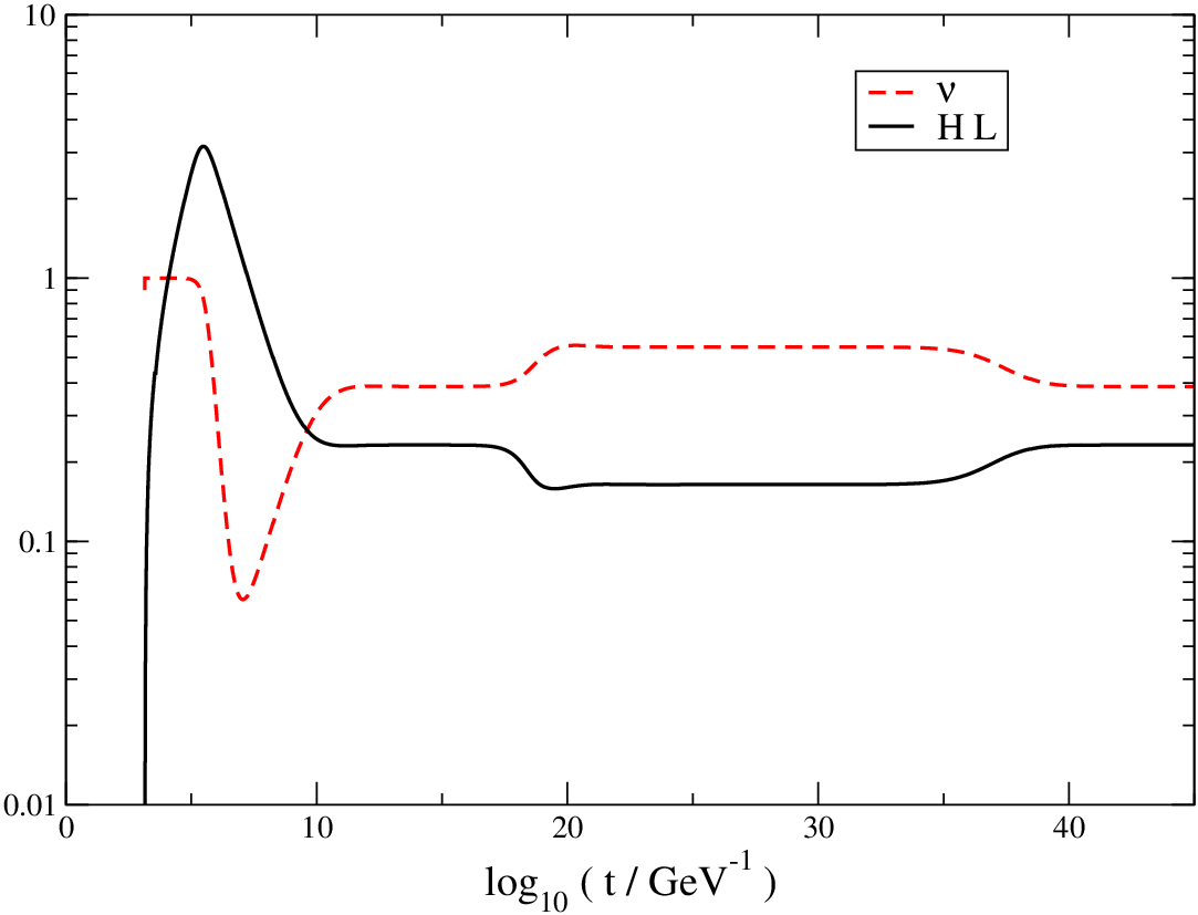
In Figs. 10 and 11 we show the numerical solutions of the string network equations for the model parameter values , , and . For comparison with Section 2, this choice corresponds to a value of . Fig. 10 depicts the evolution of the densities of the five lowest winding modes in terms of the quantities
| (4.15) |
where is the ratio of the energy density of string species relative to the critical density , and is the tension of string species . Normalizing by the tension makes proportional to times a quantity that is independent of the winding number. In Fig. 11 we show the evolution of the universal length scale and universal string velocity .
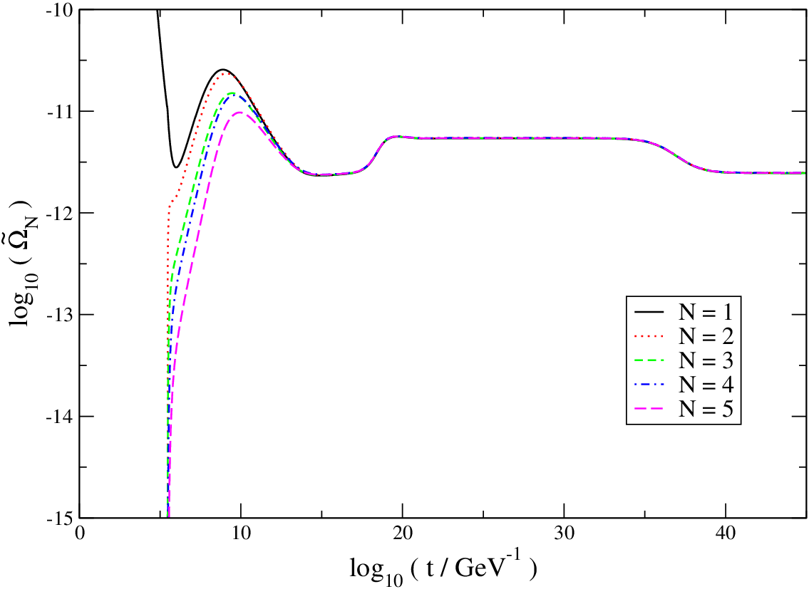
Figs. 10 and 11 show that (within the TWW model) the string energy densities approach a scaling solution at late times as evidenced by , , and all flowing to constant values. The scaling length, velocity, and densities are largely independent of the initial state of the string network. At late times, the string densities make up a nearly fixed fraction of the total energy density of the universe. We also find that the early era of oscillation dominance during reheating does not alter the final string densities in an appreciable way. These features are very similar to what is found in simulations of ordinary (abelian Higgs) string networks with only a single string species [5, 6].
The interesting new feature in the evolution of flat-direction cosmic strings is that nearly all string species flow towards very similar scaling values. This is the result of string zippering, which allows the formation of higher winding modes from lower ones. Note that the formation of these higher modes does not begin immediately. With the initial values specified above, the initial string length scale is much smaller than its scaling value, which is close to the horizon scale. This has the effect of rapidly driving the string speed to its maximal value, , at the outset, as can be seen in Fig. 11, which effectively shuts off string zippering. Once and settle down to near their scaling values, zippering begins and the higher winding-mode densities quickly flow towards their scaling values. This scaling behavior is quite robust. Changing the values of and does not alter the qualitative string densities provided is larger than the mean string velocity in the scaling regime.
The fact that many string species flow towards equal scaling values complicates the numerical analysis, since numerical limitations allow us to include only a finite number of winding modes up to an unphysical maximal value . In making Figs. 10 and 11 we have set . We also find that the final, nearly universal scaling density of the strings depends on the artificial value of . This feature is illustrated in Fig. 12. To a good approximation, the near-universal string scaling density goes like
| (4.16) |
as illustrated by the dotted line in Fig. 12. Evidently, the string energy density gets spread out among the many string types. There is also the question of how to handle the zippering of strings whose winding numbers sum to greater than . In principle, these strings can zipper into modes with which are not included in the simulation. In Figs. 10 and 11 and in the analyses to follow, we simply disallow all such zippering processes. This leads to slight increase in the scaling density of modes with . However, we have also studied other prescriptions for handling these zippering events, and for the examples we looked at, we find qualitatively similar results for the modes with .

The dependence of the scaling densities on is clearly unphysical. We would like to take , but this has its own problems. Since the energy density at large goes like (from the logarithmic dependence of the tension on the winding number), if all string species flow towards a universal scaling density proportional to the total network energy density goes like
| (4.17) |
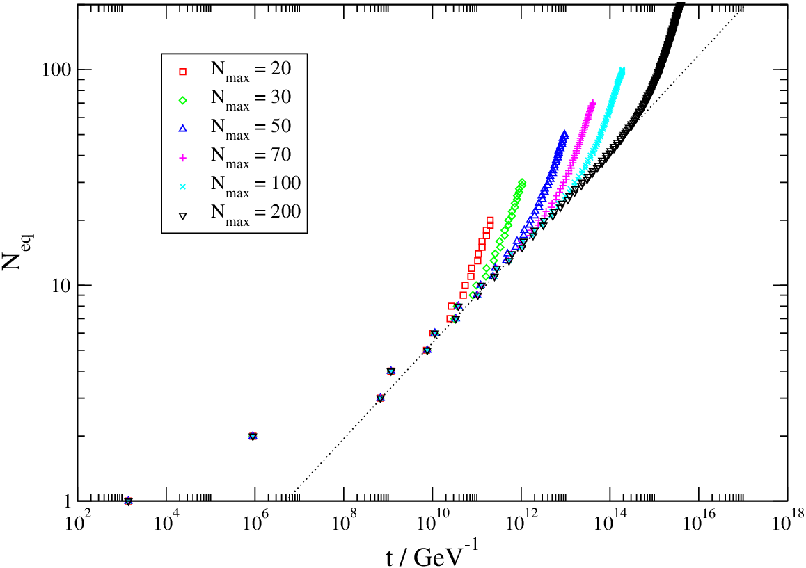
This diverges logarithmically as . In practice, however, this divergence is not realized. The initial string spectrum consists almost entirely of the lowest modes, the density of higher modes is built up from the lower modes by zippering, and these higher modes take longer to reach their scaling values. At any given time, only a finite number of strings have developed their scaling density.77 7 In this sense, our use of the term scaling for flat strings is somewhat more general than its meaning for ordinary cosmic strings because the string densities are not completely static, but very slowly varying. Let us define as the highest mode that has reached scaling by time . Modes with all have densities well below their equilibrium scaling values. Thus, at time , we effectively have , and the total energy contained in the string network goes like .
In Fig. 13 we show the time evolution of for several values of . All other parameters are the same as in Figs. 10. The curves for different values of match up for , but start to deviate from each other as the winding number approaches . Focusing on the apparently universal portion of these curves, the rate of increase of with time goes like . If we can extrapolate this dependence to much larger winding numbers, the value of at the present time will be
| (4.18) |
where we have used and . This is a very large number, but it is not so large so as to be problematic. Recall that the string tension, given in Eq. (2.63), increases logarithmically with the winding number. The tension of a string with is merely
| (4.19) |
for and , corresponding to in Eq. (2.63). Moreover, the total string energy density in the network is less than about times the energy density of a network containing a single type of string with the same tension as the lowest mode. These values for the maximal tension and the total string density are not much larger than for an ordinary cosmic string, and they present no obvious cosmological difficulties.
In our analysis of flat-direction string network evolution described above we have used a very simple analytic model of string network evolution; we have made specific assumptions about the details of the string interactions; and, we have made extrapolations into regions well beyond what we are able to probe analytically and numerically. Nevertheless, a simple picture for the evolution of a flat-direction string network emerges from our results, and is likely to be genuine, even if some of the underlying assumptions are not necessarily rigorous and the model used to study the network evolution is overly simple. In this picture, a very large number of string species reach similar scaling densities by the present time. The total energy of the network is within an order of magnitude or two of the energy density that a single abelian Higgs string species would have for the same value of the string tension. However, instead of being concentrated within a single species, the string energy density is nearly uniformly distributed among all the string species that have attained scaling. Thus, the flat-direction string network consists of a near continuum of string species, but with global properties that closely resemble those of a single species network.
Our argument for this picture is based on the very slow dependence of the flat-direction string tensions on the winding number. On account of this slow variation, the macroscopic properties of the many species that have attained scaling are very similar to each other. For example, Fig. 2 shows that the tension of a mode with is only about times that of the mode for . From this feature, as long as the zippering is reasonably efficient and the lowest mode is able to attain a scaling value for its density, we expect the densities of the string modes to be very similar to one another up to large values of the winding number .
One curious aspect of this picture is that the total energy density in the network corresponds to less than a few hundred individual strings of horizon length. It is therefore curious that the TWW model applied to flat-direction strings predicts that there are many more string species than this in the scaling regime at the present time, each with a characteristic length scale of horizon size. We suggest that the scaling densities predicted by the TWW model for flat-direction strings should be interpreted as time-averaged values. At any given epoch in the scaling regime, there exist many fewer long strings than . However, these strings are continually zippering into other string species, and averaged over time, many more string species are populated (with a lower density per string) than are present at any one time. It is also possible that this issue of discreteness leads to a value of that is smaller than what is predicted by the TWW model.
A definite confirmation of this picture of flat-direction string evolution would appear to require a full numerical simulation of the network (as well as lattice simulations to determine the zippering probabilities). This task is complicated by the need to include many different string species in the simulation, and is beyond the scope of this paper. We have, however, examined the effect of changing some of our assumptions about string zippering encoded in the coefficients , defined in Eq. (4.2). For example, we find that reducing the probability for zippering into relative to does not significantly alter the final scaling densities. We have also looked into modifying the interaction terms in Eq. (4.11), as suggested in Ref. [35], and we again find the same qualitative picture of string network evolution. These results suggest that the picture of flat string evolution presented here is robust.
Before moving on, let us briefly compare our near-continuum picture of flat-direction cosmic strings to the cosmological picture of surperstring cosmic strings derived in Ref. [32]. These quasi-fundamental strings can be labelled by pairs of integers with . A string state is stable only if and are relatively prime. States with not relatively prime can be formed but are only marginally stable. They are expected to decay into lower, stable modes after they are created. In the analysis of Ref. [32], this additional dissipative channel led to a rapid decrease in the relative population of higher-tension modes. That superstring cosmic strings do not form a near-continuum scaling network is also not surprising given that the tensions of these strings increase fairly rapidly with the mode numbers [32],
| (4.20) |
where is the superstring coupling.88 8 This formula applies in ten-dimensional flat space. It may receive corrections in other backgrounds [62]. Hence, even though flat-direction cosmic strings and strings can both form stable winding modes through zippering, these two varieties of cosmic strings interact and evolve in significantly different ways.
5 String Signatures
If cosmic strings are present in the early universe they can give rise to a number of observable signatures. No evidence for cosmic strings has been found in the temperature power spectrum of the cosmic microwave background or in large-scale sky surveys. This implies the constraint , fairly independently of the underlying string model [63, 64, 65, 66, 67]. Beyond these limits, the most promising signatures for ordinary (abelian Higgs) cosmic strings are gravitational lensing and gravitational radiation [2, 3]. We find that these signals can be modified for flat-direction cosmic strings. Flat-direction cosmic strings are also more likely to radiate into their constituent particles than ordinary cosmic strings, leading to new classes of potential signatures. By combining observations of several different phenomena, it may be possible to distinguish flat-direction cosmic strings from ordinary cosmic strings as well as cosmic superstrings.
5.1 Gravitational and Particle Radiation from Loops
Cosmic strings emit gravitational radiation primarily through the oscillations of string loops. For both ordinary and flat-direction cosmic strings, a single loop is expected to emit gravitational radiation with power
| (5.1) |
where is a dimensionless constant whose precise value depends on how the loop is oscillating [69, 70, 71, 72, 73]. This rate is independent of the length of the loop, . The radiation frequencies do depend on and are
| (5.2) |
with the relative power going into mode decreasing at least as quickly as for simple string loop solutions [70, 71, 72, 73].
To compute the gravitational wave background from a cosmic string network, one must convolute the power emitted by individual loops with the loop density distribution. Unfortunately, even for ordinary cosmic strings, the loop density distribution is not fully understood. The main uncertainty is the size of loops when they are formed. It is standard to parametrize the typical initial loop length according to
| (5.3) |
where is the time of loop formation, and estimates for range between the string width [8], to with [74, 75, 76], all the way up to [77]. We will consider different values of below.
Cosmic string loops can also radiate directly into particles [78, 79, 80]. This can arise both through the direct emission of particles from smooth strings [78, 79, 80], as well as from cusp annihilation [81]. For the string loops present in the early universe, cusp annihilation is usually the more important source of particle emission [81].99 9 This conclusion can change if there exist light (superstring) moduli fields with masses much smaller than , where is the width of the string [79, 80]. For flat direction strings, both the string width and the typical moduli mass are set by the scale of supersymmetry breaking . As a result, the rate of moduli emission by flat-direction strings is suppressed, and the corresponding bounds [82] are not relevant. A cusp is a point on a string that reaches the speed of light at some instant during its (Nambu-Goto) evolution. Cusps are a generic feature of many simple solutions for the motion of a string loop, where they are found to occur about once per oscillation period [70, 3]. In the region near the cusp, the string segments fold back upon themselves such that the separation between the adjacent segments becomes smaller than the string width. This allows these string segments to annihilate each other. Cusps should not be confused with string kinks, which are points on a string where the tangent vector changes substantially over a very short distance, on the order of the string width [73]. Unlike at a cusp, there need not be any significant annihilation of the string segments in the vicinity of a kink, and kinks can persist for many loop oscillations [83]. Kinks can be created from string reconnection and zippering.
The effective length of the overlap region between the adjacent string segments near a string cusp on a loop of length is about
| (5.4) |
where is the string width [84]. The overlapping string segments near the cusp are expected to annihilate, transferring most of the string energy within the overlap region to the constituent particles making up the string. The total average power released into particles through this process by a single string loop is [84]
| (5.5) |
Here, is the cusp rate, where corresponds to the period of a loop oscillation, and is the probability per period for a cusp to occur. We expect , although it has been argued that the presence of kinks on strings could push it to smaller values [73]. This is yet another uncertainty associated with the structure of cosmic strings on small scales.
For a given tension, flat-direction strings are much wider than ordinary cosmic strings; compared to . The amount of string annihilated in a cusp is therefore greatly enhanced. The total particle radiation power from cusp annihilation by a flat-direction string loop is
| (5.6) |
Relative to the gravitational radiation power, Eq. (5.1), we see that cusp annihilation dominates for sufficiently small loop sizes. The loop size at which the two powers become equal is
| (5.7) |
Recall that the loop size at formation is . For the loops will decay primarily through particle emission, and not gravitational radiation. On the other hand, when , most of the loop energy will go into gravity waves, except for a small burst of particles towards the end of the loop’s existence.
Thus, the emission of particles by flat-direction cosmic strings through cusp annihilation is greatly enhanced relative to ordinary cosmic strings. If cusp annihilation dominates over gravitational radiation, many of the gravitational radiation signals will be suppressed compared to ordinary cosmic strings. In order to compare the relative signals from gravitational radiation and particle emission, it is helpful to concentrate on three particular epochs in the early universe: the reheating time ; the time at which ; and the earliest time at which a given gravitational wave frequency mode can form.
We found in Section 4 that reheating after thermal inflation occurs when , where is the decay rate of the light flat-direction scalar field. This yields
| (5.8) |
Recall that if the process of reheating after thermal inflation is to avoid disturbing the predictions of nucleosynthesis, we must have for and , and for and .
The second moment of interest, the time after which newly-formed loops lose most of their energy in the form of gravity waves, occurs when . This corresponds to the time
| (5.9) | |||||
We have expressed in terms of rather than the VEV because it is this dimensionless combination that appears frequently in the estimates below. An approximate conversion between and is (see Fig. 1)
| (5.10) |
Given the upper bound on from reheating after thermal inflation, we will mostly focus on .
The third time of interest is , the earliest moment at which a given gravitational wave frequency as low as can be emitted. Recall that loops formed at time have the initial size , and subsequently shrink and radiate into frequencies . For a mode observed at the present time with frequency emitted at time , the initial frequency was
| (5.11) |
Combining these facts, the earliest time at which a mode with present frequency could have been emitted is
| (5.12) | |||||
Both and depend on the parameter that characterizes the typical size of a string loop when it is formed, . The dynamics of loop formation are not completely understood, and as a result, estimates for vary widely. Some recent simulations find that a significant portion of the loops formed are quite large, with [85, 86] or [77]. Other simulations find that the typical initial loop size approaches their resolution limits [8]. In this case, it is thought that gravitational radiation will smooth out very small fluctuations, and impose a lower limit on [3]. The scale over which this smoothing occurs is also under ongoing investigation. Early estimates suggested [3], but more recent analyses have found even smaller values of . In Ref. [74] the authors obtain with during the radiation era and during matter dominance. The authors of Ref. [75] find with in the radiation era and in the matter era. Furthermore, in Ref. [76] it is suggested that the simulation results of Ref. [77] should be interpreted as predicting a network with - of the loop energy density in the form of large loops with and the remainder in the form of very small loops with with . On account of the rapidly evolving state of the field, we will consider both large and small values of below.
Fig. 14 shows , , and in units as functions of the VEV for large loops with . The model parameters were set to , , , . In this plot we also indicate the present time and the matter-radiation equality time with dotted lines. The value of is shown for two values of the frequency, and . These values span most of the range relevant for gravitational wave searches. For these large loops, is always much less than , and all loops formed after will decay predominantly into gravitational radiation. At the lower frequency , lies below but above , and is never much less than . This suggests that the gravitational wave signal at this frequency will not be attenuated much by the enhanced rate of particle emission by the loops. On the other hand, the value of for lies well below both and , indicating that the high-frequency gravitational wave signal will be reduced.

The values of , , and for very small loops, , are shown in Fig. 15 as a function of the VEV . This value of corresponds to the estimate of Ref. [75] for loops emitted in the matter era. Even smaller values of are suggested in Ref. [74]. As before, the other model parameters were taken to be , , , and , and the dotted lines denote the present time and the matter-radiation equality time . This figure indicates that the prospects for gravitational radiation from small flat-direction string loops are much less promising than for large loops. Indeed, is larger than the present time for . Such small loops will decay almost entirely to particles instead of gravitational radiation. Even when is less than , the curves for show that the gravitational wave signal is very suppressed relative to the signal from large loops. At low frequencies there is no signal at all since exceeds the present time ; the loops are simply too small to radiate into this frequency range. Even for frequencies near , there will be a gravitational wave signal only for . Despite the reduction in the gravitational wave signal, small loops may be observable through their copious emission of particles.

In summary, we find that the large width of flat-direction cosmic strings greatly enhances the rate at which they decay into their constituent particles through cusp annihilation. With this enhancement, our preliminary analysis indicates that string loops that are initially large () decay predominantly into gravitational waves, while very small loops () decay primarily into particles. The typical size of string loops when they are formed is an unresolved problem, and well-motivated arguments in favor of large loops, very small loops, or possibly both at once, can be found in the literature. In the face of this uncertainty, we will focus on two particular choices of the loop size parameter to estimate the observational signatures from flat-direction cosmic strings. To compute the gravitational wave signals we will set for all loops, as suggested in Ref. [77]. Our results can be rescaled appropriately when only a fraction of the loops are large. To estimate the signals from particle emission due to cusp annihilation, we will instead assume that is sufficiently small that all loops decay mostly into particles. This is plausible for flat-direction strings for which the rate of particle emission by cusp annihilation is enhanced. Again, it is straightforward to modify our results to accommodate larger values of .
Finally, let us also mention that the picture of loop formation by flat-direction strings might be different from that of ordinary cosmic strings. For example, the enhanced rate of particle emission by cusp annihilation could potentially smooth out small fluctuations over scales larger than the (naïve) gravitational radiation scale . String loops can also remain bound to the parent string, as illustrated in Fig. 8. This could modify the distribution of initial string loop sizes. The rate of cusp formation on these bound loops may also be different from that on free loops.
5.2 Gravitational Wave Signatures
Cosmic strings can give rise to two types of gravitational wave signals. The combination of many string loop decays produces a smooth stochastic background of gravitational radiation [69]. On top of this background, individual cusps can produce intense bursts of gravity waves [87]. Gravitational wave detectors are sensitive to both types of signals. For the string tensions of interest, , the stochastic background is the more promising one [88, 89, 90] and we will focus on it. To estimate this gravitational wave background due to flat-direction cosmic strings we will assume that all string loops are large when they are formed, with [77]. If only a fraction of the loops produced are large, as advocated in Ref. [76], our results can be rescaled by this fraction.
We compute the gravitational radiation density due to cosmic string decays following Ref. [72]. Consider radiation in the frequency range observed today that was emitted at time . Keeping track of only the lowest mode,1010 10 In Ref. [91] this was shown to be a good approximation for computing the stochastic background. this radiation was emitted by loops of size , where
| (5.17) |
Loops of this size at time were formed at the earlier time given by
| (5.18) |
over the time range
| (5.19) |
These relations follow from the loop evolution equation , valid for and .
The rate at which loops are formed during the string scaling regime can be estimated using the results of numerical simulations or from simple analytic models like the one presented in Section 4. These predict a net energy flux into loops of
| (5.20) |
where
| (5.21) |
with , and being the scaling energy density of long strings. This result can be obtained by summing Eq. (4.11) over all string species that have equilibrated. It follows that the rate per unit volume that loops of initial size are formed is
| (5.22) |
Applying this result to loops formed in the time range , the number density of loops radiating into the frequency range of interest at time is
| (5.23) |
The redshift factor in this expression accounts for the dilution of the loops as they evolve from to . Given that each loop radiates gravity waves with a power , we can combine everything and sum over to find the signal. The total gravitational wave density at the present frequency is
| (5.24) | |||||
Here, is the critical density, and and are functions of defined by Eqs. (5.17) and (5.18). The integration limits range between and , where is given in Eq. (5.12).1111 11 Normally the lower limit would simply be , but in the present case the flat-direction string network only reaches scaling at . Numerically, we find that this additional cutoff has no visible effect because the gravity waves emitted shortly after the end of thermal inflation are diluted away during the subsequent reheating. Gravity waves from the phase transition [92] will also be diluted by thermal inflation. Noting that during the matter era ( and ) and during the radiation era (), this equation can be integrated straightforwardly. Relative to the treatment of Ref. [72], we have included a cutoff of through a step function. This accounts for the loops only being able to radiate efficiently into gravity waves if their length is greater than . It is this cutoff, along with the additional redshifting that occurs during reheating after thermal inflation, that suppresses the gravitational wave signal from flat-direction strings compared to ordinary strings.

In Fig. 16 we show the stochastic gravitational wave signal from initially large cosmic string loops as a function of frequency. We have used the parameter values , , , and in making this plot. The solid lines show the gravitational wave density from flat-direction cosmic strings, including the cutoff and the additional redshifting during reheating after thermal inflation. The dashed lines indicate what the signal would be for ordinary cosmic strings, without the cutoff or reheating effects. At lower frequencies the relevant loops are formed later on, at times greater than and , and there is no change to the signal. At higher frequencies, the cutoff on the loop size and the additional dilution during reheating both suppress the gravitational wave signals. As can be seen in Fig. 14, the cutoff is more important for lower values of (and ), while the reheating dilution is more significant at larger values of since is larger. This is why the shape of the high frequency cutoff changes as we increase .
The attenuation of high frequency gravitational wave signals is relevant to LIGO and Advanced LIGO, which can potentially probe down to at frequencies around [93]. Fig. 16 indicates that LIGO is not expected to be able to find evidence for flat-direction cosmic strings. On the other hand, the prospects for discovery at LISA and from measurements of pulsar timing are quite promising. The LISA probe is expected to cover portions of the range down to [94]. Since the gravitational wave signal from large flat-direction string loops is mostly unmodified in this frequency range, LISA will be able to probe a sizeable portion of the model parameter space. Limits from pulsar timing are currently in the frequency range [95], which is again low enough that the gravitational wave signal from flat-direction cosmic strings is unsuppressed. From this bound we obtain the constraint . It is expected that this limit will be improved to by upcoming experiments [95]. Note that flat-direction cosmic strings offer the interesting possibility that LISA and pulsar timing experiments could detect a stochastic gravitational wave background with , while (Advanced) LIGO sees nothing even though it is sensitive to signals at this level. This would be a suggestive hint for flat-direction cosmic strings.
5.3 Particle Emission Signatures: Dark Matter
Having studied the gravitational wave signatures of string loops that are large when they are formed, let us now consider the possibility that the typical initial loop size is very small, , as suggested in Refs. [74, 75]. If is sufficiently small, nearly all the energy of a loop is released as particle excitations of the fields making up the string. This is plausible for flat-direction cosmic strings due to their enhanced rate of particle emission by cusp annihilation relative to ordinary cosmic strings. In the models of flat-direction strings presented in Section 2, the fields making up the string consist of two chiral supermultiplets and one massless vector (gauge) supermultiplet. When the chiral supermultiplets develop VEVs, it is more convenient to describe the theory in terms of a heavy massive vector supermultiplet, with mass on the order of , as well as a light supermultiplet with mass on the order of [44]. This light multiplet is light on account of the flatness of the potential. Cusp annihilation will produce both the heavy and the light states making up the string. These particles will subsequently decay, and can be a potential source of dark matter and high energy cosmic rays. We consider both of these possible signatures in turn, assuming that all string loops are very small and decay entirely into particles rather than gravitational waves.
To compute the dark matter density from decaying string loops we again make use of Eq. (5.20) that specifies the rate at which the scaling string network transfers its energy into loops. Contributions to the dark matter density from loops produced before the network attains scaling are diluted away by the subsequent reheating process.1212 12 We have verified this using the simulation of Section 4. We assume that a fraction of the energy emitted by the cusp annihilations of loops eventually becomes dark matter (such as a neutralino or gravitino LSP).1313 13 The decay products from a cusp annihilation are typically boosted by factor of [84]. This can lead to values of if most of the cusp energy goes to kinetic energy rather than non-relativistic dark matter. For small initial loop sizes, , this boost is weak enough that the dark matter decay products quickly reach kinetic equilibrium for , when most of the dark matter is produced. The total dark matter density at the present time from the strings is then
| (5.25) |
where is the present time and is the time at which the DM particles freeze out of equilibrium. The factor of accounts for the additional dilution of the dark matter (or the constituent string fields) after they are produced. It is convenient to split the integration into three pieces: , , and . These integrations are straightforward and yield
| (5.26) | |||||
where is the prefactor appearing in Eq. (4.5). Numerically, the largest contribution comes from the third term, from the integration range . We have bounded the logarithm in this term from above in making this estimate. For reasonable values of the model parameters, the amount of dark matter produced by decaying loops is safely small, although smaller values of are preferred. This differs from the much stronger constraints on regular cosmic strings that are able to decay into dark matter [96], which is due to the dilution from reheating after thermal inflation.
There is an additional contribution to the DM density from the out-of-equilibrium decays of the oscillating flat-direction fields during reheating. If a small fraction of these decays ends up as dark matter, the present contribution to the DM energy density will be
| (5.27) |
Parametrizing and using , we find
| (5.28) |
Thus, the branching fraction into DM particles must be very small. Note that and can be very different from each other. The particles emitted from a cusp annihilation can include some of the heavier component fields making up the string. On the other hand, the decays of the flat-direction fields after thermal inflation involve only the light modes. The decays of these states into superpartners (such as a neutralino or heavier gravitino LSP) can therefore be highly suppressed or kinematically inaccessible, allowing for .
5.4 Particle Emission Signatures: Visible Matter
In addition to dark matter, the decays of very small string loops can produce hadrons, leptons, and photons. This particle injection will be spread out over time as the scaling string network continually rids itself of excess energy by forming loops. Visible particles created by loop decays can imprint themselves upon the early universe in a number of ways. The energetic products from loop decays at temperatures below can disrupt the predictions of big-bang nucleosynthesis (BBN). At later times, energetic photons from loop decays can modify the blackbody spectrum of the cosmic microwave background (CMB). Some of the decay products from string loops can also be highly energetic, producing ultra-high-energy cosmic rays and contributing to the extragalactic diffuse gamma-ray background. We consider the possible signatures from cosmic strings from each of these effects. As for our dark matter estimates, we assume that all loops are so small that they decay entirely into particles.
To estimate the effects of decaying string loops on BBN we make use of the results of Ref. [97]. In this work the authors used the successful predictions of BBN to place limits on the combination for a long-lived particle of mass , relic density (per unit entropy) , and lifetime , decaying at time . In contrast to a long-lived relic particle whose decays can be treated as being instantaneous, cosmic string loops are produced and decay continuously. These decays therefore have a cumulative effect on the light element abundances. To obtain a limit for decaying string loops we interpret the bounds from Ref. [97] as limits on the total energy injected within a comoving volume, , where is the total entropy within the volume .
The total energy injected into the comoving volume by string loops that decay during the time interval is
| (5.29) | |||||
In writing this expression, we have implicitly assumed that and both lie within the era of radiation dominance, as is relevant for BBN. The strongest limits on energy injection from BBN come from the relative fractions of deuterium and lithium-6 relative to hydrogen. Both of these are formed at times later than . Since the visible decay products from the loops thermalize quickly relative to the Hubble time, we set to find the bounds due to the deuterium and lithium-6 abundances [97]. Assuming a hadronic branching fraction of order unity, the total energy injection per unit entropy must be less than .1414 14 The bound is fairly independent of the mass of the decaying particle. This bound is satisfied provided .
Late-time energy injection is also constrained by the the nearly perfect blackbody spectrum of the CMB observed by COBE/FIRAS [98]. Photons produced by the decays of string loops that occur after the time can distort this spectrum. Before , double Compton scattering () efficiently thermalizes any additional photons that are created. The precise form of the spectral distortions created after depends on the time at which the photons were injected. However, the net constraint from the non-observation of such distortions can be reduced to a constraint on the total photon energy created after , [99, 100, 101]. The net photon injection from decaying string loops can be estimated using the rate of energy deposition by the network. If all the energy injected is in the form of photons (possibly after cascading), the total injection is
| (5.30) | |||||
Numerically, the dominant contribution to the injected photon energy comes from the most recent era, , leading to a non-zero value for the Compton parameter [100, 102] which quantifies deviations away from the black body spectrum. It is expected that the constraints on photon injection will be improved in the future by the ARCADE experiment [103].
Decaying cosmic string loops can also generate cosmic rays. The corresponding energy spectrum depends on the energies of the particles emitted in the loop decays. Recall that the fields making up the flat-direction strings consist of a light chiral supermultiplet and a heavy massive vector supermultiplet. In each cusp annihilation, both the heavy and the light states can be produced. The decays of the heavy states, with masses on the order of , can generate ultra-high-energy cosmic rays (UHECR) [104]. Decays of the light states, with masses on the order of , contribute to the extragalactic diffuse gamma-ray background (EDGRB) [105]. To determine the relevant bounds and prospects, we will assume that the energy released in each cusp annihilation goes initially into a fraction of the light states (with soft energy) and a fraction to the heavy states. We expect , with possibly smaller.
The contribution of decaying string loops to the EDGRB was studied in Ref. [105]. Data from the EGRET experiment [106] constrains the rate of energy emission into the light scalar states with masses on the order of (that decay into lower-energy gamma rays) at the present time to . Equating this bound with Eq. (5.20) evaluated at the present time, we obtain the bound [105]
| (5.31) |
This does not represent a significant constraint beyond those found above. The heavy component states making up the string can also contribute to the EDGRB through the photons they produce in cascade decays. The limit in this case is about the same as from the decays of the light states given in Eq.(5.31), but with replaced by . These constraints from the gamma-ray background on decaying cosmic string loops will be strengthened by the upcoming GLAST experiment [107]. However, the range of the model that can be probed may ultimately be limited by astrophysical background contributions to the gamma-ray flux.
Ultra-high-energy cosmic rays can be produced by cusp annihilation if some of the heavier states making up the string are created. When the heavy states decay, their products are highly energetic, making them a source of high-energy neutrinos and UHECRs. Estimates of the UHECR flux for strings that decay into particles were made in Ref. [108] and are directly applicable to flat-direction cosmic strings. These authors find that for energies greater than about , the only relevant cosmic ray flux consists of neutrinos. The fluxes of highly energetic protons and photons are very suppressed because they are attenuated by their interactions with the cosmic background. Extrapolating the predictions of Ref. [108], the neutrino signal from decaying strings can be probed directly at Ice Cube [109] down to in the energy range -. The Auger project is sensitive to UHECR showers induced by energetic neutrinos in the energy range - [110]. The Auger measurements imply the constraint
| (5.32) |
For , this corresponds to .
Our analysis indicates that the visible matter signatures from decays of flat-direction string loops are consistent with observations provided is small enough. However, there is another visible matter signature that is challenging to reproduce in models of flat-direction strings, namely the baryon asymmetry of the universe. Flat-direction strings are formed following a period of thermal inflation. The typically low reheating temperature after thermal inflation, Eq. (4.6), combined with the large amount of dilution from the inflationary expansion and reheating imply that baryogenesis mechanisms that operate at or above the electroweak scale will no longer work. Instead, the baryon asymmetry must be produced at very late times. This can arise from the strings themselves [111, 112, 113], from the non-thermal production of particles during reheating that have baryon-number violating decays [57, 114, 115, 116, 117], or by the Affleck-Dine mechanism [118].
5.5 String Loops and Zero Modes
In our discussion of radiation from cosmic string loops, we implicitly assumed that there do not exist any zero mode excitations along the strings. Zero modes are fermionic or bosonic field fluctuations with vanishing energy that are localized on the string. The existence of zero modes on cosmic strings can alter the picture of loop radiation in important ways [119, 120, 121, 122].
These undamped, particle-like excitations can be excited when a string loop is formed. As the loop radiates and shrinks, the number density of the zero modes builds up. Eventually the angular momentum of the zero modes balances the tendency of the loop to shrink, and a quasi-stable loop remnant, or vorton, is left over. If such vortons are sufficiently long-lived and numerous, they behave like quasi-stable matter and can further modify the predictions of BBN or create too much dark matter. The presence of vortons typically leads to extremely strong constraints on the underlying field theory [122].
For the flat-direction strings we are studying, fermionic zero modes [123, 119] are of particular relevance. It was shown in Ref. [21, 22] that such modes are a generic feature of supersymmetric cosmic string solutions. In the present case, we also have supersymmetry breaking operators present in the Lagrangian. We find that adding a supersymmetry breaking gaugino mass destroys all the fermionic zero modes. A recent study also suggests that more generally, fermionic zero modes do not form on closed string loops at all [124]. The existence of bosonic zero modes depends on the other fields in the theory and their couplings, and are less generic [119]. We do not consider them here.
Zero modes, either bosonic or fermionic, are also unlikely to stabilize flat-direction cosmic strings simply because these strings are relatively wide. For the phase transition leading to flat-direction cosmic strings, we expect that the radius at which the zero modes would stabilize a string loop, if they were to exist, is usually much smaller than the width of the string [19]. As discussed above for cusp annihilation, when the separation between a pair of antiparallel string segments approaches the string width these segments will annihilate into their constituent fields, and the loop will decay before stabilizing as a vorton.
5.6 Lensing by Cosmic Strings
While an indirect gamma ray or gravitational wave signal from cosmic strings would be exciting, ideally one would like a direct observation to confirm their existence. This can be achieved by observing gravitational lensing by a string. The primary gravitational effect of the large mass density contained within a cosmic string is to modify the surrounding spacetime such that it is flat, but with a deficit angle of [125]. When light from a galaxy passes by a (non-relativistic) cosmic string, the deficit angle produces a distinctive double image with an angular separation of [3, 125]
| (5.33) |
where is the distance from the lensing string to the source galaxy, is the distance from the observer to the source, and is the angle between the string axis and the line-of-sight. From a single lensing event it is possible to determine directly, as well as by measuring the redshift of the source. Given that a single string lensing event is found, it is likely that the same string will also lens the images of other galaxies that are nearby on the sky [126]. By observing several galaxies lensed by the same string, the tension of that string can be determined [127].
The gravitational lensing signatures from flat-direction strings are even richer than those of ordinary strings because of the stability of higher winding modes. If many lensed images from different strings are observed, it may be possible to measure tensions of several strings and obtain clues about the mass spectrum of the higher winding modes. In this respect, flat-direction cosmic strings are similar to cosmic superstrings. Both types of cosmic strings also have junctions connecting different winding modes. These can produce triple images, in addition to the double images produced by a lone string [128]. Since the spectrum of tensions of flat-direction strings is very different from that of strings, the observation of many gravitational lensing events might allow one to distinguish between them. Unfortunately, the probability of observing a lensed image from a flat-direction string is very small due the indirect bounds on the tension, . This is smaller than the expected sensitivity of from upcoming optical surveys [129], and from the SKA [130], radio survey [131]. The results of Ref. [127] also suggest that it will be difficult to determine the string tension accurately enough to distinguish between flat-direction string winding modes with similar values of the winding number .
6 Conclusion
We conclude by summarizing some of our findings:
- •
Abelian gauge symmetry breaking along a flat direction can give rise to strongly Type-I cosmic strings with tension , gauge profile width of and scalar profile width , where characterizes the flatness of the potential. These flat-direction strings are likely to be formed after thermal inflation through flux-trapping.
- •
The tension of the strings increases very slowly with their winding number . Thus, higher-winding mode strings are energetically stable. This enables strings to be attracted to one another and zipper, creating stable formations with winding number or , where and are the original string winding numbers.
- •
Zippering affects the evolution of the resulting string network. Applying a simple network evolution model to flat-direction strings suggests that a large number of string modes develop roughly equal densities in the early universe. The total energy density is about the same as for a single string, but it is distributed among many species.
- •
Flat-direction strings radiate gravitationally. However, in contrast to ordinary cosmic strings, they also may be able to radiate copiously into matter. The strings are expected to fully radiate away, as there is no vorton obstruction for the supersymmetric flat-direction strings under consideration.
- •
In contrast to GUT strings, flat-direction strings are generically compatible with current direct observational constraints, [63, 64, 65, 66, 67]. If the typical initial loop length is close to the horizon scale, LISA and upcoming millipulsar timing probes may be able to detect the gravitational wave signal from these strings. However, the gravity wave signal at higher frequencies is suppressed for flat-direction strings, making their detection at LIGO extremely challenging.
- •
Particle emission from cusp annihilation is likely to be the dominant loop decay mechanism if the loop length is always much smaller than the horizon. This intriguing prospect for flat-direction cosmic strings entertains the possibility that ultra-high-energy cosmic rays or nonthermal dark matter originate from their particle emission. If all loops decay entirely into particles, the constraints from BBN, the CMB blackbody, and UHECRs imply the bound , corresponding to .
- •
The multi-tension network of flat-direction strings formed in the early universe is in contrast to the standard single-tension string networks, but similar to cosmic superstring networks, and thus may mimic the latter by giving rise to multiple lensing events. However, the spectrum of tensions of flat-direction strings is constrained by indirect bounds, and may be too low to be observed in the near future.
We find that flat-direction cosmic strings behave in ways that are qualitatively different from both ordinary (abelian Higgs) cosmic strings as well as cosmic superstrings. These differences in behavior may be distinguishable through probes of the early universe.
Acknowledgements
We thank L. Bettencourt, D. Chung, A. Pierce, E. Rozo, and K. Turzynski for helpful conversations, and N. Arkani-Hamed for pushing us to look more closely at the boosted decay products from cusps. This work was supported by the National Science Foundation under Grant No. PHY-0456635, the Department of Energy, and the Michigan Center for Theoretical Physics (MCTP).
References
- [1] H. B. Nielsen and P. Olesen, Nucl. Phys. B 61, 45 (1973).
- [2] M. B. Hindmarsh and T. W. B. Kibble, Rept. Prog. Phys. 58, 477 (1995) [hep-ph/9411342].
- [3] A. Vilenkin and E. P. S. Shellard, Cosmic Strings and Other Topological Defects, Cambridge University Press, Cambridge UK, 1994.
- [4] T. W. B. Kibble, J. Phys. A 9, 1387 (1976).
- [5] D. P. Bennett and F. R. Bouchet, Phys. Rev. Lett. 60, 257 (1988); D. P. Bennett and F. R. Bouchet, Phys. Rev. D 41, 2408 (1990).
- [6] B. Allen and E. P. S. Shellard, Phys. Rev. Lett. 64, 119 (1990).
- [7] C. J. A. Martins and E. P. S. Shellard, Phys. Rev. D 53, 575 (1996) [hep-ph/9507335]; C. J. A. Martins and E. P. S. Shellard, Phys. Rev. D 54, 2535 (1996) [hep-ph/9602271]; C. J. A. Martins and E. P. S. Shellard, Phys. Rev. D 65, 043514 (2002) [hep-ph/0003298].
- [8] G. R. Vincent, M. Hindmarsh and M. Sakellariadou, Phys. Rev. D 56, 637 (1997) [astro-ph/9612135]; G. Vincent, N. D. Antunes and M. Hindmarsh, Phys. Rev. Lett. 80, 2277 (1998) [hep-ph/9708427].
- [9] V. Vanchurin, K. D. Olum and A. Vilenkin, Phys. Rev. D 74, 063527 (2006) [gr-qc/0511159].
- [10] For reviews, see for example H. E. Haber and G. L. Kane, Phys. Rept. 117, 75 (1985); S. P. Martin, [hep-ph/9709356]; D. J. H. Chung et al., Phys. Rept. 407, 1 (2005) [hep-ph/0312378]; M. A. Luty, [hep-th/0509029].
- [11] R. Blumenhagen, M. Cvetic, P. Langacker and G. Shiu, Ann. Rev. Nucl. Part. Sci. 55, 71 (2005) [hep-th/0502005]; P. Langacker, hep-ph/9805486; P. Langacker and J. Wang, Phys. Rev. D 58, 115010 (1998) [hep-ph/9804428]; J. R. Espinosa, Nucl. Phys. Proc. Suppl. 62, 187 (1998) [hep-ph/9707541]; M. Cvetic and P. Langacker, Phys. Rev. D 54, 3570 (1996) [hep-ph/9511378]; M. Cvetic and P. Langacker, Mod. Phys. Lett. A 11, 1247 (1996) [hep-ph/9602424].
- [12] P. Langacker, N. Polonsky and J. Wang, Phys. Rev. D 60, 115005 (1999) [hep-ph/9905252]; D. Suematsu, Phys. Rev. D 59, 055017 (1999) [hep-ph/9808409].
- [13] C. T. Hill, H. M. Hodges and M. S. Turner, Phys. Rev. D 37, 263 (1988).
- [14] K. Freese, T. Gherghetta and H. Umeda, Phys. Rev. D 54, 6083 (1996) [hep-ph/9512211].
- [15] T. Barreiro, E. J. Copeland, D. H. Lyth and T. Prokopec, Phys. Rev. D 54, 1379 (1996) [hep-ph/9602263].
- [16] A. A. Penin, V. A. Rubakov, P. G. Tinyakov and S. V. Troitsky, Phys. Lett. B 389, 13 (1996) [hep-ph/9609257].
- [17] W. B. Perkins and A. C. Davis, Phys. Lett. B 428, 254 (1998) [hep-ph/9803303].
- [18] A. Yung, Nucl. Phys. B 562, 191 (1999) [hep-th/9906243]; K. Evlampiev and A. Yung, Nucl. Phys. B 662, 120 (2003) [hep-th/0303047]; M. Shifman and A. Yung, [hep-th/0703267].
- [19] S. C. Davis, P. Binetruy and A. C. Davis, Phys. Lett. B 611, 39 (2005) [hep-th/0501200].
- [20] M. Donaire and A. Rajantie, Phys. Rev. D 73, 063517 (2006) [hep-ph/0508272].
- [21] S. C. Davis, A. C. Davis and M. Trodden, Phys. Lett. B 405, 257 (1997) [hep-ph/9702360].
- [22] S. C. Davis, A. C. Davis and M. Trodden, Phys. Rev. D 57, 5184 (1998) [hep-ph/9711313].
- [23] M. Endo, M. Kawasaki and T. Moroi, Phys. Lett. B 569, 73 (2003) [hep-ph/0304126].
- [24] R. Jeannerot, J. Rocher and M. Sakellariadou, Phys. Rev. D 68, 103514 (2003) [hep-ph/0308134]. J. Rocher and M. Sakellariadou, JCAP 0503, 004 (2005) [hep-ph/0406120]. J. Rocher and M. Sakellariadou, Phys. Rev. Lett. 94, 011303 (2005) [hep-ph/0412143].
- [25] P. Laguna and R. A. Matzner, Phys. Rev. Lett. 62, 1948 (1989).
- [26] L. M. A. Bettencourt and T. W. B. Kibble, Phys. Lett. B 332, 297 (1994) [hep-ph/9405221].
- [27] L. M. A. Bettencourt, P. Laguna and R. A. Matzner, Phys. Rev. Lett. 78, 2066 (1997) [hep-ph/9612350].
- [28] E. J. Copeland and N. Turok, “Cosmic String Interactions,”, FERMILAB-PUB-86-127-A (1986).
- [29] See for example, E. P. S. Shellard, Nucl. Phys. B 283, 624 (1987).
- [30] R. A. Matzner, Comput.Phys. 2, 51 (1988).
- [31] A. Achucarro and R. de Putter, Phys. Rev. D 74, 121701 (2006) [hep-th/0605084].
- [32] S. H. Tye, I. Wasserman and M. Wyman, Phys. Rev. D 71, 103508 (2005) [Erratum-ibid. D 71, 129906 (2005)] [astro-ph/0503506].
- [33] E. J. Copeland and P. M. Saffin, JHEP 0511, 023 (2005) [hep-th/0505110].
- [34] L. Leblond and M. Wyman, Phys. Rev. D 75, 123522 (2007) [astro-ph/0701427].
- [35] A. Avgoustidis and E. P. S. Shellard, [0705.3395 [astro-ph]].
- [36]
For a review of cosmic strings from superstring theory, see:
J. Polchinski, [hep-th/0412244]. - [37] N. T. Jones, H. Stoica and S. H. H. Tye, JHEP 0207, 051 (2002) [hep-th/0203163]; S. Sarangi and S. H. H. Tye, Phys. Lett. B 536, 185 (2002) [hep-th/0204074]. N. T. Jones, H. Stoica and S. H. H. Tye, Phys. Lett. B 563, 6 (2003) [hep-th/0303269].
- [38] G. Dvali and A. Vilenkin, JCAP 0403, 010 (2004) [hep-th/0312007].
- [39] E. J. Copeland, R. C. Myers and J. Polchinski, JHEP 0406, 013 (2004) [hep-th/0312067].
- [40] J. Polchinski, AIP Conf. Proc. 743, 331 (2005) [Int. J. Mod. Phys. A 20, 3413 (2005)] [hep-th/0410082].
- [41] M. G. Jackson, N. T. Jones and J. Polchinski, JHEP 0510, 013 (2005) [hep-th/0405229].
- [42] E. J. Copeland, R. C. Myers and J. Polchinski, Comptes Rendus Physique 5, 1021 (2004).
- [43] A. Hanany and K. Hashimoto, JHEP 0506, 021 (2005) [hep-th/0501031].
- [44] D. E. Morrissey and J. D. Wells, JHEP 0701, 102 (2007) [hep-ph/0606234].
- [45] S. P. Martin, Phys. Rev. D 61, 035004 (2000) [hep-ph/9907550].
- [46] C. H. Taubes, Commun. Math. Phys. 72, 277 (1980).
- [47] L. M. A. Bettencourt and R. J. Rivers, Phys. Rev. D 51, 1842 (1995) [hep-ph/9405222].
- [48] J. M. Speight, Phys. Rev. D 55, 3830 (1997) [hep-th/9603155].
- [49] L. Jacobs and C. Rebbi, Phys. Rev. B 19, 4486 (1979).
- [50] K. J. M. Moriarty, E. Myers and C. Rebbi, Phys. Lett. B 207, 411 (1988).
- [51] E. Myers, C. Rebbi and R. Strilka, Phys. Rev. D 45, 1355 (1992).
- [52] A. Rajantie, M. Sakellariadou and H. Stoica, [0706.3662 [hep-th]].
- [53] E. J. Copeland, T. W. B. Kibble and D. A. Steer, Phys. Rev. Lett. 97, 021602 (2006) [hep-th/0601153]; E. J. Copeland, T. W. B. Kibble and D. A. Steer, [hep-th/0611243].
- [54] G. Lazarides, C. Panagiotakopoulos and Q. Shafi, Phys. Rev. Lett. 56, 557 (1986).
- [55] K. Yamamoto, Phys. Lett. B 168, 341 (1986).
- [56] D. H. Lyth and E. D. Stewart, Phys. Rev. D 53, 1784 (1996) [hep-ph/9510204].
- [57] K. Yamamoto, Phys. Lett. B 194, 390 (1987).
- [58] S. Hannestad, Phys. Rev. D 70, 043506 (2004) [astro-ph/0403291].
- [59] K. Ichikawa, M. Kawasaki and F. Takahashi, Phys. Rev. D 72, 043522 (2005) [astro-ph/0505395].
- [60] A. Rajantie, Int. J. Mod. Phys. A 17, 1 (2002) [hep-ph/0108159].
- [61] J. J. Blanco-Pillado, K. D. Olum and A. Vilenkin, [0706.1577 [hep-th]].
- [62] H. Firouzjahi, L. Leblond and S. H. Henry Tye, JHEP 0605, 047 (2006) [arXiv:hep-th/0603161].
- [63] M. Wyman, L. Pogosian and I. Wasserman, Phys. Rev. D 72, 023513 (2005) [Erratum-ibid. D 73, 089905 (2006)] [astro-ph/0503364].
- [64] A. A. Fraisse, JCAP 0703, 008 (2007) [astro-ph/0603589].
- [65] L. Pogosian, I. Wasserman and M. Wyman, [astro-ph/0604141].
- [66] U. Seljak, A. Slosar and P. McDonald, JCAP 0610, 014 (2006) [astro-ph/0604335].
- [67] N. Bevis, M. Hindmarsh, M. Kunz and J. Urrestilla, Phys. Rev. D 75, 065015 (2007) [astro-ph/0605018]; N. Bevis, M. Hindmarsh, M. Kunz and J. Urrestilla, [astro-ph/0702223].
- [68] R. A. Battye, B. Garbrecht and A. Moss, JCAP 0609, 007 (2006) [astro-ph/0607339]; R. A. Battye, B. Garbrecht, A. Moss and H. Stoica, [0710.1541 [astro-ph]].
- [69] A. Vilenkin, Phys. Lett. B 107, 47 (1981).
- [70] N. Turok, Nucl. Phys. B 242, 520 (1984).
- [71] C. J. Burden, Phys. Lett. B 164, 277 (1985).
- [72] T. Vachaspati and A. Vilenkin, Phys. Rev. D 31, 3052 (1985).
- [73] D. Garfinkle and T. Vachaspati, Phys. Rev. D 36, 2229 (1987).
- [74] X. Siemens and K. D. Olum, Nucl. Phys. B 611, 125 (2001) [Erratum-ibid. B 645, 367 (2002)] [gr-qc/0104085]. X. Siemens, K. D. Olum and A. Vilenkin, Phys. Rev. D 66, 043501 (2002) [gr-qc/0203006].
- [75] J. Polchinski and J. V. Rocha, Phys. Rev. D 74, 083504 (2006) [hep-ph/0606205]; J. Polchinski and J. V. Rocha, Phys. Rev. D 75, 123503 (2007) [gr-qc/0702055].
- [76] J. Polchinski, [0707.0888 [astro-ph]].
- [77] V. Vanchurin, K. Olum and A. Vilenkin, Phys. Rev. D 72, 063514 (2005) [gr-qc/0501040]; V. Vanchurin, K. D. Olum and A. Vilenkin, Phys. Rev. D 74, 063527 (2006) [gr-qc/0511159]; K. D. Olum and V. Vanchurin, Phys. Rev. D 75, 063521 (2007) [astro-ph/0610419].
- [78] M. Srednicki and S. Theisen, Phys. Lett. B 189, 397 (1987).
- [79] T. Damour and A. Vilenkin, Phys. Rev. Lett. 78, 2288 (1997) [gr-qc/9610005].
- [80] M. Peloso and L. Sorbo, Nucl. Phys. B 649, 88 (2003) [hep-ph/0205063].
- [81] R. H. Brandenberger, Nucl. Phys. B 293, 812 (1987).
- [82] E. Babichev and M. Kachelriess, Phys. Lett. B 614, 1 (2005) [hep-th/0502135].
- [83] J. M. Quashnock and D. N. Spergel, Phys. Rev. D 42, 2505 (1990).
- [84] J. J. Blanco-Pillado and K. D. Olum, Phys. Rev. D 59, 063508 (1999) [gr-qc/9810005], K. D. Olum and J. J. Blanco-Pillado, Phys. Rev. D 60, 023503 (1999) [gr-qc/9812040].
- [85] C. Ringeval, M. Sakellariadou and F. Bouchet, JCAP 0702, 023 (2007) [astro-ph/0511646].
- [86] C. J. A. Martins and E. P. S. Shellard, Phys. Rev. D 73, 043515 (2006) [astro-ph/0511792].
- [87] T. Damour and A. Vilenkin, Phys. Rev. D 64, 064008 (2001) [gr-qc/0104026], T. Damour and A. Vilenkin, Phys. Rev. D 71, 063510 (2005) [hep-th/0410222].
- [88] X. Siemens, J. Creighton, I. Maor, S. Ray Majumder, K. Cannon and J. Read, Phys. Rev. D 73, 105001 (2006) [gr-qc/0603115].
- [89] C. J. Hogan, Phys. Rev. D 74, 043526 (2006) [astro-ph/0605567].
- [90] X. Siemens, V. Mandic and J. Creighton, [astro-ph/0610920].
- [91] M. R. DePies and C. J. Hogan, Phys. Rev. D 75, 125006 (2007) [astro-ph/0702335].
- [92] C. Grojean and G. Servant, Phys. Rev. D 75, 043507 (2007) [hep-ph/0607107].
- [93] B. Abbott et al. [LIGO Scientific Collaboration], Astrophys. J. 659, 918 (2007) [astro-ph/0608606].
- [94] http://lisa.nasa.gov
- [95] F. A. Jenet et al., Astrophys. J. 653, 1571 (2006) [astro-ph/0609013].
- [96] R. Jeannerot, X. Zhang and R. H. Brandenberger, JHEP 9912, 003 (1999) [hep-ph/9901357].
- [97] M. Kawasaki, K. Kohri and T. Moroi, Phys. Rev. D 71, 083502 (2005) [astro-ph/0408426].
- [98] D. J. Fixsen, E. S. Cheng, J. M. Gales, J. C. Mather, R. A. Shafer and E. L. Wright, Astrophys. J. 473, 576 (1996) [astro-ph/9605054].
- [99] R. H. Brandenberger, B. Carter and A. C. Davis, Phys. Lett. B 534, 1 (2002) [hep-ph/0202168].
- [100] W. Hu and J. Silk, Phys. Rev. D 48, 485 (1993).
- [101] K. Hagiwara et al. [Particle Data Group], Phys. Rev. D 66, 010001 (2002).
- [102] T. Kanzaki, M. Kawasaki, K. Kohri and T. Moroi, [0705.1200 [hep-ph]].
- [103] A. Kogut et al., New Astron. Rev. 50, 925 (2006) [astro-ph/0609373].
- [104]
P. Bhattacharjee,
Phys. Rev. D 40, 3968 (1989),
J. H. MacGibbon and R. H. Brandenberger, Nucl. Phys. B 331, 153 (1990). - [105] P. Bhattacharjee, Q. Shafi and F. W. Stecker, Phys. Rev. Lett. 80, 3698 (1998) [hep-ph/9710533].
- [106] P. Sreekumar et al. [EGRET Collaboration], Astrophys. J. 494, 523 (1998) [astro-ph/9709257].
- [107] E. D. Bloom [GLAST team Collaboration], Space Sci. Rev. 75, 109 (1996).
- [108] U. F. Wichoski, J. H. MacGibbon and R. H. Brandenberger, Phys. Rev. D 65, 063005 (2002) [hep-ph/9805419].
- [109] K. Filimonov [IceCube Collaboration], AIP Conf. Proc. 870, 215 (2006), J. Becker [IceCube Collaboration], J. Phys. Conf. Ser. 60, 219 (2007).
- [110] P. Facal San Luis [Pierre Auger Collaboration], [0706.4322 [astro-ph]].
- [111] M. Kawasaki and K. i. Maeda, Phys. Lett. B 208, 84 (1988) [Phys. Lett. B 209, 271 (1988)].
- [112] M. Mohazzab, Phys. Lett. B 350, 13 (1995) [arXiv:hep-ph/9409274].
- [113] I. Dasgupta, Phys. Rev. D 55, 3318 (1997) [arXiv:hep-ph/9604356].
- [114] G. Lazarides, C. Panagiotakopoulos and Q. Shafi, Phys. Lett. B 183, 289 (1987); G. Lazarides, C. Panagiotakopoulos and Q. Shafi, Nucl. Phys. B 307, 937 (1988).
- [115] S. Dimopoulos and L. J. Hall, Phys. Lett. B 196, 135 (1987).
- [116] J. Cline and S. Raby, Phys. Rev. D 43, 1781 (1991).
- [117] K. S. Babu, R. N. Mohapatra and S. Nasri, Phys. Rev. Lett. 97, 131301 (2006) [hep-ph/0606144]; K. S. Babu, R. N. Mohapatra and S. Nasri, Phys. Rev. Lett. 98, 161301 (2007) [hep-ph/0612357].
- [118] E. D. Stewart, M. Kawasaki and T. Yanagida, Phys. Rev. D 54, 6032 (1996) [hep-ph/9603324]; G. N. Felder, H. Kim, W. I. Park and E. D. Stewart, JCAP 0706, 005 (2007) [hep-ph/0703275].
- [119] E. Witten, Nucl. Phys. B 249, 557 (1985).
- [120] B. Carter, Phys. Lett. B 238, 166 (1990) [hep-th/0703023].
- [121] R. H. Brandenberger, B. Carter, A. C. Davis and M. Trodden, Phys. Rev. D 54, 6059 (1996) [hep-ph/9605382].
- [122] A. C. Davis, [hep-ph/0305008].
- [123] R. Jackiw and P. Rossi, Nucl. Phys. B 190, 681 (1981).
- [124] M. Postma and B. Hartmann, [0706.0416 [hep-th]].
- [125] A. Vilenkin, ApJ, 282, L51 (1984)
- [126] D. Huterer and T. Vachaspati, Phys. Rev. D 68, 041301 (2003) [astro-ph/0305006].
- [127] M. Oguri and K. Takahashi, Phys. Rev. D 72, 085013 (2005) [astro-ph/0509187].
- [128] B. Shlaer and M. Wyman, Phys. Rev. D 72, 123504 (2005) [hep-th/0509177].
- [129] M. A. Gasparini, P. Marshall, T. Treu, E. Morganson and F. Dubath, [0710.5544 [astro-ph]].
- [130] P. Diamond and S. Rawlings, Frontiers 23, 13 (2006).
- [131] K. J. Mack, D. H. Wesley and L. J. King, [astro-ph/0702648].