Central exclusive production of scalar meson
at the Tevatron, RHIC and LHC energiesPreprint:
Abstract
We calculate several differential distributions for exclusive double diffractive production in proton-antiproton collisions at the Tevatron and in proton-proton collisions at RHIC and LHC in terms of unintegrated gluon distributions (UGDFs) within the -factorisation approach. The uncertainties of the Khoze-Martin-Ryskin approach are discussed in detail. The transition vertex is calculated as a function of gluon virtualities applying the standard pNRQCD technique. The off-shell effects are discussed and quantified. They lead to a reduction of the cross section by a factor 2–5, depending on the position in the phase space and UGDFs. Different models of UGDFs are used and the results are shown and discussed. The cross section for diffractive component depends strongly on UGDFs. We calculate also the differential distributions for the fusion mechanism. The integrated cross section for photon-photon fusion is much smaller than that of diffractive origin. The two components have very different dependence on momentum transfers in the nucleon lines as well as azimuthal-angle correlations between both outgoing nucleons.
pacs
13.87.Ce, 13.60.Le, 13.85.LgI Introduction
The discovery of Higgs is the main motivation for the construction and putting into operation the Large Hadron Collider (LHC) at CERN. The analysis of inclusive cross section will be the “main road” of the future investigations. Different decay channels will be studied. The analysis in each (!) of these channels is rather complicated as huge unreduceable backgrounds are unavoidably present.
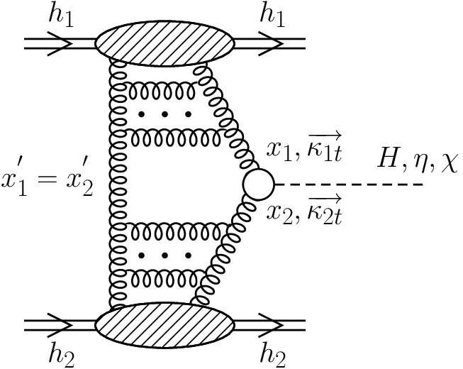
The diffractive exclusive production of Higgs boson seems to be much cleaner in this respect. Many estimates of the corresponding cross section has been presented in the literature. The so-called Durham model KMR is the state-of-art in this field. The cross section for the diffractive production is much smaller than the cross section for the inclusive case, but the ratio of the signal to more conventional background seems promising. Recently appeared a detailed analysis of diffractive production of MSSM Higgs KMR_MSSM. We do not need to mention that any check of the used theoretical methods against experimental data are not possible at present, at least for the Higgs production. The way out is to study the diffractive production of heavy quarkonia where almost the same theoretical methods can be used. The basic diagram for the amplitude of the process is shown in Fig. 1. The production of heavy quarkonia received a lot of attention from both theory and experiment in recent years. For a review we refer to Refs.Sch94; BF; Bottom; Kramer01; Brambilla.
QCD dynamics at small quark and gluon momentum fractions (or large total energy), relevant for HERA, Tevatron, RHIC and LHC, is still poorly understood. It was shown in HKSST00; LSZ02 that the combination of the -factorisation approach CCH90; CE91; CC96; RSS99 and the next-to-leading-logarithmic-approximation (NLLA) BFKL vertex FL96 gives quite good agreement with data on inclusive -production. One can therefore hope that these concepts provide a valueable foundation also for exclusive processes.
Kaidalov, Khoze, Martin and Ryskin proposed to calculate diffractive double elastic 11 1 Both protons survive the collision. production of Higgs boson in terms of unintegrated gluon distributions KMR. It is not clear at present how reliable such calculations are, and it would be interesting to apply this approach to heavy quarkonia production. In Refs. Yuan01; KMR-chi integrated cross section for exclusive double diffractive production was estimated with the identical formulae as for the scalar Higgs production with replaced by . Of course, such a procedure can be strictly right in general case only for ficticious structureless objects, when the internal wave function and gluon virtualities are neglected. From the spectroscopy point of view the meson is a quark-antiquark P-wave state, and it might be interesting to study an exclusive production of P-waves applying pNRQCD methods. Such a calculation may be especially important when we go to larger gluon virtualities.
Parallel to the exclusive channel studies there was a lot of theoretical activity for inclusive charmonium and bottomonium production; see for example HKSST01; Vasin; Likhoded. There non-relativistic pQCD methods are usually applied. In these approaches the nonrelativistic quark-antiquark wave function is taken explicitly into the calculation. The vertex function corresponds to so-called quasi multi-Regge kinematics (QMRK), i.e. when and have similar rapidities and form a cluster. It is based on the formalism developed by Lipatov and Fadin FL96 for diffractive pair production.
In the present work we shall use the pNRQCD methods for exclusive double diffractive production. The main ingredients of our calculations are the unintegrated gluon distributions (UGDFs) and the effective NLLA BFKL production vertex in QMRK (with reggeised gluon couplings to quarks). We would like to compare results obtained using this vertex with the KMR results. The projection of the heavy quark-antiquark pair onto the corresponding charmonium state is described in the standard way within the non-relativistic-quarkonium-model Guberina; Baier; Cho-Leibo. Finally, we shall refer to the KMR result KMR-chi where the wave function is not included explicitly. For completeness, we shall include also photon-photon fusion mechanism of exclusive production shown in Fig. 2. In addition to the diffractive QCD approach we discuss also a phenomenological Pomeron-Pomeron fusion approach.

In the present paper we wish to calculate differential distributions for exclusive production with different UGDFs from the literature. We shall calculate matrix elements for off-shell gluons. We shall discuss also uncertainty related to the approximation made, to the choice of the scale, etc. The contribution of the fusion to the differential cross sections will be calculated.
II Diffractive QCD mechanism
In the pNRQCD approach the diffractive exclusive reaction is viewed as shown in Fig. 3. The corresponding calculation can be summarized as follows. First, the -continuum amplitude is calculated. Then the amplitude is reduced to the amplitude with standard projection techniques developed in Guberina; Kuhn.

II.1 General kinematics of double diffractive QCD mechanism
Let’s consider first the -production. The kinematic variables for the process on the quark level is shown in Fig. 4.

We use the following definition of the light cone coordinates
where are the light-cone basis vectors. In the c.m.s. frame
| (1) |
and the momenta of the scattering hadrons are given by
where the Mandelstam variable The momenta of the t-channel gluons are , and (see Fig. 4). The on-shell quark and antiquark (with mass ) have momentum respectively with
In the high energy (large ) regime we have
where is the momentum of the heavy charmonium with mass : . The longitudinal momentum fractions of the gluons are , . Of course, we will finally assume that
The decomposition of gluon momenta into longitudinal and transverse parts gives
| (2) | |||
We take into account below that . Making use of conservation laws we get
| (3) |
Taking the transverse parts from these relations gives
| (4) |
II.2 Matrix element for exclusive double diffractive production
According to Khoze-Martin-Ryskin approach (KMR) KMR, we write the amplitude of exclusive double diffractive colour singlet production as
| (5) |
The normalization of this amplitude differs from the KMR one KMR-chi; KMR by the factor and coincides with the normalization in our previous work on exclusive -production SPT07. The amplitude is averaged over the colour indices and over two transverse polarisations of the incoming gluons KMR. The bare amplitude above is subjected to absorption corrections which depend on collision energy. We shall discuss this issue shortly when presenting our results.
The vertex factor in expression (5) describes the coupling of two virtual gluons to -meson that can be written as
| (6) |
where is the operator that projects the pair onto the charmonium bound state (see below), is the production amplitude of a pair of massive quark and antiquark with momenta , , respectively.
Within the QMRK approach FL96 we have
| (7) |
where are the colour group generators in the fundamental representation, are the effective vertices (8) arising from the Feynman rules of QMRK illustrated in Fig. (5).

| (8) | |||
Taking into account definitions (1) and (II.1) and using the gauge invariance property
we get the following projection
| (9) |
Normalization of the polarization vectors coincides with the one in Ref. Forshaw05. Since we adopt here the definition of the polarization vectors proportional to gluon transverse momenta , then we must take into account the longitudinal momenta in numerators of vertices (8). While projecting on the color singlet the -verticies in (8) cancel each other and disappear from the resulting matrix element, so there contributes only the first diagram in the decomposition in Fig. 5.
As a consequence of the gauge invariance the charmonium production amplitude for on-mass-shell quark and antiquark states obeys the following property
Projection of the hard amplitude onto the singlet charmonium bound state is given by a 4-dimentional integral over relative momentum of quark and antiquark HKSST00; HKSST01:
| (10) | |||
Here the function is the momentum space wave function of the charmonium, and the projection operator for a small relative momentum has the form
| (11) |
Factor in the formula (10) has been introduced to compensate the difference between the analogous formula in Guberina; Cho-Leibo written in 3-dimentional form. The Clebsch-Gordan coefficient in color space in our case is where factor provides the averaging of the production matrix element squared over intermediate quark states in the loop. Using that we get
| (12) | |||||
Since -wave function vanishes at the origin, we may expand the trace in (10) in a Taylor series around , and only the linear terms in in the trace (12) survive. This yields an expression proportional to
| (13) |
with the derivative of the -wave radial wave function at the origin whose numerical values can be found in EQ95. The general -wave result (10) may be further reduced by employing the Clebsch-Gordan identity which for the scalar charmonium reads
Using the relations (II.1) and and we obtain
| (14) |
that will be useful below. The longitudinal momentum fractions are now calculated as
| (15) |
Above is the rapidity of the produced meson.
Therefore, within QMRK approach we get finally the following vertex function
We have also calculated the subprocess matrix element squared that is usually used in inclusive production calculations. The form of is identical to the form of the matrix element squared obtained very recently by Likhoded and Luchinsky in Ref. Likhoded.
The objects and appearing in formula (5) are skewed (or off-diagonal) unintegrated gluon distributions. They are non-diagonal both in and space. Usual off-diagonal gluon distributions are non-diagonal only in . In the limit , and they become usual UGDFs. Our choice of different UGDFs will be discussed in more detail in a separate section.
II.3 Khoze-Martin-Ryskin approach
In the original Khoze-Martin-Ryskin (KMR) approach KMR the amplitude is written as
| (16) |
where only one transverse momentum is taken into account somewhat arbitrarily as
| (17) |
and the normalization factor can be written in terms of the decay width (see below).
In the KMR approach the large meson mass approximation is adopted, so the gluon virtualities are neglected in the vertex factor
| (18) |
In our approach we generalize the approximation taking into account corresponding off-shell effects.
The KMR UGDFs are written in the factorized form:
| (19) |
with GeV-2 KMR. In our approach we use different parametrization of the -dependent isoscalar form factors (see Eqns. (32) and (33) below).
Please note that the KMR and our skewed UGDFs have different number of arguments. In the KMR approach there is only one effective gluon transverse momentum (see Eq.(17)) compared to two idependent transverse momenta in our case (see Eq.(32)).
The KMR skewed distributions are given in terms of conventional integrated densities and the so-called Sudakov form factor as follows:
| (20) |
The square root here was taken using arguments that only survival probability for hard gluons is relevant. It is not so-obvious if this approximation is reliable for quarkonium production. In addition this has to be contrasted with the choice of gluon momentum of the KMR UGDF in (17) as minimal (not harder) of two gluons. The factor approximately accounts for the single skewed effect KMR. Please note also that in contrast to our approach the skewed KMR UGDF does not explicitly depend on (assuming ). Usually this factor is estimated to be 1.3–1.5. In our evaluations here we take it to be equal 1 to avoid further uncertainties.
In contrast to the Higgs case, in the case of light quarkonium production rather small values of gluon transverse momenta give the dominant contribution to the integral (16). Therefore it becomes essential what one does phenomenologically in the nonperturbative region , where the is a minimal nonperturbative scale for standard integrated distributions. Of course, formally for scales smaller than the standard collinear gluon distributions do not exist and an extra extension is unavoidable. This issue was not discussed in detail in the literature. We shall illustrate this point in the result section.
The Sudakov factor is the result of resumming the virtual contributions in the DGLAP evolution and reads
| (21) |
with . In their (KMR) estimates the hard scale is usually taken . Of course the choice of the scale is somewhat arbitrary, and the consequences of this choice were not discussed in the literature.
In Fig.6 we show the KMR distribution (20) as a function of for different values of specified in the figure for two different choices of the scale. The DGLAP distribution for is not well defined and we arbitrarily put it to zero as in Ref.KMR-chi. In principle, one could try several other extrapolations into the nonperturbative region to see its influence on the resulting differential cross sections.


II.4 Our vertex versus Khoze-Martin-Ryskin vertex
We wish to compare our vertex function (II.2) with the KMR vertex function KMR-chi. In the KMR limit of large meson mass and the vertex reads
| (22) | |||||
Following now the KMR notations KMR-chi we write the total NRQCD QMRK amplitude (5) (averaged over colour and polarisation states of incoming gluons) in the limit as
| (23) |
where the normalization is
| (24) |
and the vertex factor is defined in (18).
Normalization constant can be obtained in another way in terms of the partial decay width as (see formula (19) in the KMR paper KMR-chi)
| (25) |
Using the expression for , obtained in the framework of pNRQCD Cakir; Close
| (26) |
we get the normalization constant (with )
| (27) |
which coincides with the normalisation of the vertex factor obtained within the QMRK approach (24).
Therefore, in the leading order the QMRK approach is in agreement with the KMR approach in the limit of large meson mass . We shall discuss deviations from this approximation due to the off-shell effects in the result section. Similar analysis of off-shell effects was performed recently for inclusive Higgs production in Ref. PTS06.
II.5 Off-diagonal UGDFs and choice of scales
In the present work we shall use a few sets of unintegrated gluon distributions which aim at the description of phenomena where small gluon transverse momenta are involved. Some details concerning the distributions can be found in Ref. LS06. We shall follow the notation there.
The larger energies, the smaller values of parton momentum fractions come into game. Therefore at larger energies we shall use distributions constructed exclusively for small values of . Two of them are based on the idea of gluon saturation. One of them was obtained based on a saturation-inspired parametrization of the dipole-nucleon cross section which leads to a good description of the HERA data GBW_glue. The second one KL01 was constructed to describe the inclusive RHIC pion spectra. The third one is the asymptotic BFKL distribution BFKL. We do not wish to repeat more details here. It can be found in individual references as well as in Ref. LS06 where applications of UGDFs to correlations was discussed.
Due to its simplicity the Gaussian smearing of initial transverse momenta is a good reference point for other approaches. It allows to study phenomenologically the role of transverse momenta in several high-energy processes. We define simple unintegrated gluon distribution
| (28) |
where are standard collinear (integrated) gluon distribution and is a Gaussian two-dimensional function
| (29) |
The UGDF defined by Eq. (28) and (29) are normalized such that
| (30) |
The UGDFs have the following property
| (31) |
if 0. The small- region is of nonperturbative nature and is rather modelled than derived from pQCD.
The two-scale off-diagonal distributions require a separate discussion. In the general case we do not know UGDFs very well. It seems reasonable, at least in the first approximation, to take in the amplitude (5)
| (32) |
where and are isoscalar nucleon form factors DL
| (33) |
and and are total four-momentum transfers in the first and second proton line, respectively. The proton form factor in the form (33) gives rather good description of the -dependence of the elastic cross section at high energies, i.e. for kinematics similar as in our case. The above prescription for UGDFs (32) is a bit arbitrary, although it is inspired by the positivity constraints for collinear Generalized Parton Distributions posit. It provides, however, an interpolation between different and values. Our prescription is more symmetric in variables of the first and second exchange than the one used in Ref. BBKM06 for Higgs boson production.
The choice of the (factorisation) scales here is not completely obvious too. We shall try the following three choices:
| (34) | |||||
The first choice is similar as in Ref. KMR; KimbMR. However, it is not obvious if the scale associated with the “hard” production () can be used for the left part of the gluonic ladder where no obvious hard scale appears. Therefore we shall try also the second choice where we shall use = 0.26 GeV2, i.e. the nonperturbative input for the QCD evolution in Ref. GRV. Another option was proposed by Lonnblad and Sjödahl in Ref. Lonnblad. They take as a first scale. In our case this prescription must be supplemented by freezing the scale for gluon transverse momenta smaller than (minimal perturbative scale).
III fusion mechanism
As stated in the introduction we wish to investigate the competition of the diffractive QCD mechanism discussed in the previous sections and the -fusion mechanism shown in more detail in Fig. 7.

III.1 NRQCD approach
In the most general case the Born amplitude reads
| (35) | |||||
where the sign stands for -scattering and the sign for -scattering. In the following we have omitted the spin-flipping contributions related to the respective Pauli form factors. Limiting to large energies () and small momenta transfer () the matrix element for reaction via -fusion can be written as
| (36) |
where and are Dirac proton electromagnetic form factors, and the vertex has analogous form as (10)
| (37) | |||
and Repeating similar steps as for diffractive production we get
| (38) | |||
For example, in the case of scalar meson we have
| (39) |
This amplitude can be rewritten in the general gauge invariant form PTS06 in terms of two independent form factors
| (40) |
where
From this amplitude the standard decay width follows
| (41) |
So the normalization of the amplitude (40) is correct.
Analogously with the diffractive case (II.1) let us define the photon transverse momenta. Momentum conservation dictates us the following decompositions of photon momenta into longitudinal and transverse parts
| (42) |
where . Due to the gauge invariance we have similarly to (9)
| (43) |
In the relevant limit we get finally the following matrix element for reaction via -fusion
| (44) |
where and is the relative angle between photons (or outgoing protons). The amplitude (44) is purely imaginary, so there is no interference with diffractive process describing by purely real amplitude (5). This amplitude will be used in the following to calculate differential cross section.
III.2 Equivalent Photon Approximation
In the equivalent photon approximation (EPA) the total cross section for can be written as a convolution of EPA flux factors and the resonant cross section
| (45) |
The elementary cross section can be written in terms of partial decay width as
| (46) |
Let us introduce two new variables:
| (47) |
Now the cross section can be written as
| (48) |
Integrating over invariant mass of the two photons we get
| (49) |
where now
| (50) |
This equation is suitable to calculate distribution of in the Feynman variable . The analytical flux factors of photons in protons of Drees and Zeppenfeld DZ89 are taken. We have also tried:
| (51) |
where . The decay width from PDG PDG06 is = 0.2626 10-5 GeV.
IV Pomeron-Pomeron fusion
Above we have shown how to calculate the diffractive meson production mechanism in a QCD-inspired approach. Often in the literature in order to describe the high-energy processes one uses a phenomenological object known as pomeron. Often a vector nature is prescribed to such an object, i.e. it is assumed that it couples to the nucleons or (quarks) via matrices, i.e. similarly as photon. The corresponding mechanism for exclusive meson production is sketched in Fig.8.

The amplitude for our exclusive process may be written as
| (52) |
In the equation above are so-called Regge propagators. They can be written as:
| (53) |
are form factors describing helicity-preserving coupling of the pomeron to the nucleon. We take them to be identical to the Dirac electromagnetic form factors of the proton. Such a choice is justified by the phenomenology of elastic proton-proton scattering (see e.g.DL). The pomeron coupling to the charm quark and/or antiquark is reduced compared to the coupling to the nucleon () by the factor 3 (three quarks in the nucleon versus single charm quark/antiquark) and extra factor (heavy quark interaction is weaker than light quark interaction). This parameter can be extracted from the inelastic interaction of with the nucleons in nuclei KMR-chi. In the Tevatron energy 0.2. The parameters of the pomeron exchanges: and are taken from the Donnachie-Landshoff fits to the proton-proton and proton-antiproton total cross sections DL92. The vertex can be obtained from the vertex by replacing charm quark charge by unity.
The comparison of the results with pomeron-pomeron fusion with the diffractive QCD results will be given in the result section.
V Cross section and phase space
The cross section for the 3-body reaction can be written as
| (54) |
The three-body phase space volume element reads
| (55) |
At high energies and small momentum transfers the phase space volume element can be written as
| (56) |
where , are longitudinal momentum fractions carried by outgoing protons with respect to their parent protons and the relative angle between outgoing protons . Changing variables one gets
| (57) |
It is more convenient for lower (but still high) energy to use variable . However, at very high energies the cross section becomes too much peaked at 0 due to the jacobian
| (58) |
and the use of rapidity instead of is recommended. The phase space element in this case has the following simple form
| (59) |
If is used then
| (60) |
In the other case when the meson rapidity is used then
| (61) |
Now the four-momentum transfers in both proton lines can be calculated as
| (62) |
Only if = 1, . The latter approximate relation was often used in earlier works on diffractive production of particles. However, in practice 0 and the more exact equation must be used. The range of and is not unlimited as it is often assumed. One can read off from Eq.(62) a kinematical upper limit for which is
| (63) |
In practice these phase space limits become active only for 0.2. The lower limits are energy dependent but are not active in practice.
VI Results
In Ref.KMR-chi estimates of the integrated cross sections were given. We wish to concentrate on differential distributions. Before we show our results we wish to discuss uncertainties related to the KMR approach.
VI.1 Uncertainties in the KMR approach
In the KMR approach only one effective transverse momentum is taken explicitly in their skewed unintegrated distributions. In the KMR prescription it is the minimum of the transverse momenta of the two gluons connected to the same proton line. In order to see the uncertainties related to such a choice we shall present results obtained with the following, equally arbitrary, choices:
- •
1) ,
- •
2) ,
- •
3) .
- •
4) ,
- •
5) .
As an example in Fig.9 we show results for the Feynman distribution. As can be seen from the figure there are rather large uncertainties related to the choice of the effective transverse momentum.

The estimate by Khoze, Martin, Ryskin and Stirling in Ref.KMR-chi was done for one selected value of the hard scale in the KMR UGDF . In Fig.10 we show the dependence of the differential cross section on the value of the scale. There is a sizeable effect (about a factor of two) on the cross section (see also Table 1 with integrated cross sections). For 0, the smaller the bigger the cross section.

In order to demonstrate sensitivity to the nonperturbative region of small transverse momenta in Fig.11 we show results with the KMR UGDF cut off for small values of the effective gluon transverse momenta . One observes a rather strong dependence on the value of the cut-off parameter. The bigger the value of the cut-off parameter the smaller the cross section. The results for the integrated cross section are summarized in Table I. Even for large values of the cut-off parameter ( 1 GeV2) sizeable cross sections are obtained.

The estimate in Ref.KMR-chi was done assuming that the gluons in the vertex are on mass shell, which is exact only in the infinite meson mass limit. In this paper (see subsection IIB) we take into account the effect of gluon virtualities. In Fig.12 we show the role of the off-shell effects for the KMR UGDF. The off-shell effect leads to a reduction of the cross section by a factor of 2 – 5.

Finally we show the influence of the off-shell effects on azimuthal-angle correlation function. The off-shell effect in the matrix element reduces the cross section but does not change its shape. The shape of the distribution requires an extra comment. The distribution in azimuthal angle is very different from as expected for one-step fusion (e.g. photon-photon, pomeron-pomeron fusion) to be discussed in detail in the next subsection.

VI.2 Our approach
In Fig.14 we present our distributions of the mesons in the Feynman variable . We present results obtained with different UGDFs. Characteristic for central diffractive production all distributions peak at 0. Although all UGDFs give a similar quality description of the low- HERA data for the structure function, they give quite different longitudinal momentum distributions of at the Tevatron energy = 1960 GeV. The UGDFs which take into account saturation effects (GBW, KL) give much lower cross section than the BFKL UGDF (dash-dotted line). Similar as in Ref.SPT07 rather small values of ’s in formula (5) come into the game here. Therefore the process considered here would help, at least in principle, to constrain the poorly known UGDFs.


In Fig.15 we show distributions in the square of the four-momentum transfers ( or ) in the nucleons lines. Because they are identical we shall denote them for brevity. The distributions shown in the figure are peaked at small values of or . Slightly different slopes are obtained with different UGDFs. This demonstrates how purely known are UGDFs at present. The measurement of such distributions requires measuring forward protons (or antiprotons). In the case no measurement of forward nucleons is possible one should study events with low multiplicity (only particles from the decay of ). This can be either pairs of pions or pairs of kaons or pairs of photons or . Unfortunately branching ratios to these channels are rather low PDG06.

In Fig.16 we show azimuthal angular correlations of the outgoing nucleons. Measuring such distribution experimentally requires identification of both nucleons in very forward/backward directions. This is not possible with the present Tevatron apparatus. We hope such a measurement will be possible with the final LHC instrumentation. All distributions shown in Fig.16 are peaked at 1800 i.e. for the back-to-back kinematics. The fact that the distributions are not simple functions (sin, cos) of the relative azimuthal angle between outgoing nucleons is due to the loop integral in Eq.(5) which destroys the dependence one would obtained with single fusion of well defined objects (mesons or reggeons).

Another type of proton-antiproton correlation is shown in Fig.17. We show results for KL and BFKL UGDFs as well as for photon-photon fusion. Finally we show the two-dimensional distribution in and for the “fusion” of two vector pomerons. The () distribution obtained in the photon-photon fusion mechanism differs qualitatively from the all other distributions. One can see a strong enhancement of the cross section when 0 or 0. Also the shape of the two-dimensional spectrum obtained for the fusion of phenomenological vector pomerons differs from those obtained in the QCD-inspired KMR mechanism (please note minimum of the cross section when 0 and/or 0).


In order to demonstrate the role of the gluon transverse momenta in UGDFs in Fig.18 we show distributions in for the Gaussian UGDF for different values of the smearing parameter . We wish to notice here that all such UGDFs correspond to identical integrated GDFs. The smaller value of the larger the cross section. This demonstrates that the main contributions to the cross section come from the region of very small transverse momenta of the t-channel gluons (see Fig.4). This is cleary the region where nonperturbative effects are dominant.


Let us turn now to the second mechanism of the exclusive production – the two-photon fusion mechanism sketched in Fig.2. In Fig.19 we show corresponding distribution in the Feynman variable . For comparison we show also the EPA result (dotted line) discussed in subsection IIIB.
For pedagogical purpose in Fig.20 we show also the result of the calculation with vector-like pomerons as described in section IV. Rather smaller cross section is obtained compared to the more QCD-inspired calculation with UGDFs. The cross section depends strongly on the value of the parameters of the form factor describing coupling of the phenomenological pomeron to nucleons. The value of = 15-20 GeV-2 is preferred from the proton-proton or proton-antiproton elastic scattering phenomenology. Compared to the calculation with UGDFs presented in Fig.14 the distribution around = 0 is much broader here. The thinner distribution in the case of the -factorization approach is due to the -dependence of the UGDFs entering the basic formula. The values of x’s (, etc.) in the off-diagonal UGDFs change quickly with the Feynman variable which makes the peak at = 0 much thinner than for the phenomenological pomeron exchange discussed here.


Let us return for a while to -distributions. In Fig.21 we show single distributions for photon-photon and Pomeron-Pomeron fusion mechanisms in (relevant for one-nucleon tagged case) obtained by projecting the two-dimensional distributions shown in Fig.17. The electromagnetic component peaks at very small values of due to the photon propagators.
The results for the diffractive mechanism depend strongly on the details of the calculation. Here we show only one distribution of diffractive component for easy reference. Although the diffractive component is subjected to much stronger absorption effects than the electromagnetic one, it is clear that the diffractive component dominates.

In Fig.22 we show differential distribution in relative azimuthal angle for and Pomeron-Pomeron fusion mechanisms. One sees a typical dependence characteristic for one-step exchanges. These distributions are very different from those shown in Fig.16 for pQCD diffraction where the underlying mechanism is more complicated due to a two-step nature of the process (see Fig.4).

Above we have calculated only bare distributions. Those are subjected to absorption effects. The absorption effects are usually included by multiplying the bare distributions by a soft gap survival probability. The gap survival probability was estimated to 0.05 and 0.025 KMR-chi. Absorption leads therefore to a large reduction of the bare cross section. In principle, the absorption effects may modify also shapes of differential distributions. This requires a further detailed analysis which goes beyond the scope of the present paper.
As discussed in this paper there are huge uncertainties in estimating the cross section for exclusive production, much larger e.g. than for the exlusive production where the corresponding amplitude can be related to the amplitude of photoproduction in collisions SS07. Only a real experiment may shed more light on the dynamics of production mechanism. Measuring centrally produced , one forward nucleon (proton or antiproton) and imposing a condition of rapidity gap in the second hemisphere should allow, at least in principle, such a measurement.
In Table I we have combined the cross section integrated over the whole available phase space for exclusive production of the mesons.
| UGDF, details | |||
| 1. KMR, GeV2, on-shell | |||
| vertex, min prescription for | 0.1357(+4) | 0.1357(+3) | 0.1357(+1) |
| 2. KMR, GeV2, on-shell | |||
| vertex, max prescription for | 0.9628(+4) | 0.9628(+3) | 0.9628(+1) |
| 3. KMR, GeV2, off-shell | |||
| vertex, min prescription for | 0.3720(+4) | 0.3720(+3) | 0.3720(+1) |
| 4. KMR, GeV2, on-shell | |||
| vertex, min prescription for | 0.8227(+3) | 0.8227(+2) | 0.8227(+0) |
| 5. KMR, GeV2, on-shell | |||
| vertex, min prescription for | 0.4124(+3) | 0.4124(+2) | 0.4124(+0) |
| 6. KMR, GeV2, on-shell | |||
| vertex, min prescription for | 0.2745(+3) | 0.2745(+2) | 0.2745(+0) |
| 4. KL, on-shell vertex | 0.1180(+3) | 0.1180(+2) | 0.1180(+0) |
| 5. KL, off-shell vertex | 0.5231(+2) | 0.5231(+1) | 0.5231(-1) |
| 6. GBW, on-shell vertex | 0.8514(+2) | 0.8514(+1) | 0.8514(-1) |
| 7. GBW, off-shell vertex | 0.1590(+3) | 0.1590(+2) | 0.1590(+0) |
| 8. BFKL, on-shell vertex | 0.2603(+4) | 0.2603(+3) | 0.2603(+1) |
| 9. BFKL, off-shell vertex | 0.1125(+4) | 0.1125(+3) | 0.1125(+1) |
| 10. Gauss, GeV, | |||
| off-shell vertex, scales (2) | 0.2141(+2) | 0.2141(+1) | 0.2141(-1) |
| 11. Gauss, GeV, | |||
| off-shell vertex, scales (2) | 0.1811(+1) | 0.1811(+0) | 0.1811(-2) |
In Table 1 we have assumed = 1960 GeV, = 0.1 and BR. The recently measured value of the branching ratio is 1.3 0.11 % PDG06. The last column shows possible contribution of the decay to the exclusive production of if the soft photon cannot be correctly identified. We get typically 0.1-5 nb, i.e. much less than the direct photoproduction SS07. It would be interesting to calculate the contribution of and , where the corresponding branching ratios are order of magnitude larger. On the other hand, within the approximations made in Ref.Yuan01 the cross sections for diffractive production of and vanish. It would be interesting to go beyond the approximations of Ref.Yuan01.
The exclusive production of has been reported recently by the CDF collaboration CDF_limit with the upper limit for the cross section
| (64) |
within the CDF experimental cuts. These numbers cannot be directly compared with our results in Table 1 that do not include the experimental cuts. Such a comparison requires a Monte Carlo type analysis as was done in Ref.RRABP07.
VI.3 Energy dependence
Up to now we have concentrated on Tevatron energy. We expect some results for exclusive production in not too distant future. It would be also interesting to measure exclusive production at different energies. The obvious choices are RHIC and LHC in the near future. In Fig.23 we show distributions in for different UGDFs for RHIC, W = 200 GeV (left panel) and LHC, W = 14000 GeV (right panel). Compared to Tevatron the distributions in for RHIC are wider and distribution for LHC are more narrow, concentrated around = 0. While at RHIC energy different UGDFs give relatively similar results, at LHC energy there is a difference of several orders of magnitude between results obtained with different UGDFs. Therefore a measurement at LHC should clearly select the best distribution.
In Table II we have collected total cross sections for selected UGDFs at RHIC, Tevatron and LHC. Comparing results for the three different energies we see that different UGDFs predict completely different energy dependence. While BFKL predicts a strong growth of the cross section with the collision energy, the saturation models (KL, GBW) predict much slower rise with the collison energy. Therefore measuring exclusive production at three different energies would be useful to pin down underlying dynamics.
| UGDF | RHIC | Tevatron | LHC |
| Kl | 0.6430(+1) | 0.5231(+2) | 0.1090(+3) |
| GBW | 0.2830(+1) | 0.1590(+3) | 0.1413(+3) |
| BFKl | 0.6140(+1) | 0.1125(+4) | 0.6306(+5) |
| Gauss, GeV, | |||
| scales (2) | 0.7126(-1) | 0.1811(+1) | 0.1428(+2) |


VII Discussion and Conclusions
In the present paper we have discussed in detail the exclusive production of the meson in proton-antiproton and proton-proton collisions. We have considered both diffractive and purely electromagnetic mechanisms. Many differential distributions have been discussed for the first time in the literature.
The diffractive component was calculated in the Khoze-Martin-Ryskin approach. Compared to the original KMR calculation we have taken into account the off-shellness of the gluons in the corresponding diagram. The corresponding matrix element was calculated. We find that the inclusion of the gluon virtualities reduces the cross section by a factor of 2 – 5, depending on kinematical region and on UGDFs.
We have discussed uncertainties in the KMR approach related to the treatment of the nonperturbative region as well as related to the choice of the scale in their skewed unintegrated distributions. This gives an uncertainty of a factor 2 – 3.
We get similar integrated cross section as in Ref.KMR-chi if we take the on-shell approximation for the vertex, make the same choice of scales, use the same integrated gluon distributions, etc. Summarizing, we find rather large uncertainties in the approach.
Many other UGDFs from the literature were also used to calculate distributions in the Feynman variable , in squares of the four-momentum transfers ( and ) in the nucleon lines and in relative azimuthal angle between outgoing protons. Also correlations in and have been analyzed. The results depend strongly on the choice of UGDF. This is related to a particular sensitivity of the cross section for the reaction under consideration to the nonperturbative region of very small gluon transverse momenta. Therfore a measurement of the differential distributions would be very helpful to test the unintegrated distributions in this region. At RHIC one could measure the and/or decay channels. Probably ALICE could use a similar method. At Tevatron rather or channels seem preferable.
In the present paper we have calculated only bare distributions. Those are subjected to absorption effects. The absorption effects are usually included by multiplying the bare distributions by a soft gap survival probability. The survival probability was estimate as 0.05 and 0.025 KMR-chi. Absorption leads therefore to a large reduction of the bare cross section. In principle the absorption effects may modify also shapes of differential distributions SS07. This requires a further detailed analysis which goes, however, beyond the scope of the present paper.
For completeness we have calculated also the cross section in a more phenomenological approach with Regge-type pomeron-pomeron fusion. Cross sections of the same order of magnitude as for the QCD approach are obtained. However, the azimuthal angle correlation functions for both approaches are very different.
We have also calculated differential distributions for the photon-photon fusion. This contribution turned out to be rather small (a fraction of nb). The differential distributions have quite different shapes compared to the diffractive component. Compared to the diffractive component it is peaked at extremely small values of and/or . Also the azimuthal angle correlations pattern is very different: for the fusion and a more complicated shape for the diffractive component due to the loop integration in the formula for the amplitude.
Recently, there is an interest at Tevatron to study exclusive production of meson. This is because of a possibility to study photoproduction at large energies SS07 and due to a potential search for odderon exchange BMSC07. Because of its decay channel and difficulties in identifying soft photons the decays may contribute to the “exclusive” production of making the measurement of photoproduction and/or the discovery of the odderon exchange difficult. A comparison of theoretical cross sections for the three mentioned reactions would be therefore very useful in this context. Our estimates for Tevatron energies, including soft survival probability, give (20 – 200) nb times = 0.013 which gives the corresponding cross section rather less than 1 nb compared to about 15 nb for the photoproduction SS07.
We have made also calculation of distributions and total cross sections for RHIC and LHC. Comparing these results and those for the Tevatron leads to the conclusion that only measurements for different energies may help to disentangle underlying QCD dynamics. In principle, such measurements could even explore the onset of QCD saturation which is not so easy to be discovered in inclusive reactions.
Acknowledgements This work was partially supported by the grant of the Polish Ministry of Scientific Research and Information Technology number 1 P03B 028 28, the Russian Foundation for Fundamental Research, grants No. 06-02-16215 and No. 07-02-91557, and the Bogoliubov-Infeld Programme 2007.
References
- (1)
V.A. Khoze, A.D. Martin and M.G. Ryskin, Phys. Lett. B 401,
330 (1997);
V.A. Khoze, A.D. Martin and M.G. Ryskin, Eur. Phys. J. C 23, 311 (2002);
A.B. Kaidalov, V.A. Khoze, A.D. Martin and M.G. Ryskin, Eur. Phys. J. C 31, 387 (2003) [arXiv:hep-ph/0307064];
A.B. Kaidalov, V.A. Khoze, A.D. Martin and M.G. Ryskin, Eur. Phys. J. C 33, 261 (2004);
V.A. Khoze, A.D. Martin, M.G. Ryskin and W.J. Stirling, Eur. Phys. J. C 35, 211 (2004). - (2) S. Heinemeyer, V.A. Khoze, M.G. Ryskin, W.J. Stirling, M. Tasevsky and G. Weiglein, arXiv:0708.3052 [hep-ph].
- (3) G.A. Schuler, CERN-TH-7170-94, hep-ph/9403387
- (4) E. Braaten, S. Fleming and T. C. Yuan, Ann. Rev. Nucl. Part. Sci. 46, 197 (1996) [arXiv:hep-ph/9602374].
- (5) Bottom Production, Proceedings of Workshop on Standard Model Physics at the LHC, Geneva, Switzerland 1999, [arXiv:hep-ph/0003142].
- (6) N. Brambilla et al. [Quarkonium Working Group], FERMILAB-FN-0779, CERN-2005-005, Dec 2004. 521pp, arXiv:hep-ph/0412158.
- (7) M. Kramer, Prog. Part. Nucl. Phys. 47, 141 (2001) [arXiv:hep-ph/0106120].
- (8)
P. Hagler, R. Kirschner, A. Schafer, L. Szymanowski and O. Teryaev,
Phys. Rev. D 62, 071502 (2000)
[arXiv:hep-ph/0002077];
Ph. Hagler, R. Kirschner, A. Schafer, L. Szymanowski and O. V. Teryaev, Phys. Rev. D 63, 077501 (2001) [arXiv:hep-ph/0008316]. - (9) F. Yuan, Phys. Lett. B510, 155 (2001).
- (10)
A.V. Lipatov, V.A. Saleev and N.P. Zotov, hep-ph/0112114;
S.P. Baranov, A.V. Lipatov and N.P. Zotov, hep-ph/0302171, Yad. Fiz. 67, 856 (2004). - (11) S. Catani, M. Ciafaloni and F. Hautmann, Phys. Lett. B242, 97(1990); Nucl. Phys. B366, 135 (1991).
- (12) J.C. Collins and R.K. Ellis, Nucl. Phys. B360, 3 (1991).
- (13) G. Camici and M. Ciafaloni, Phys. Lett. B386, 341 (1996); Nucl.Phys.B496, 305 (1997).
- (14) M.G. Ryskin, A.G. Shuvaev and Yu.M. Shabelski, hep-ph/9907507.
- (15)
V. S. Fadin and L. N. Lipatov,
Nucl. Phys. B 477, 767 (1996)
[arXiv:hep-ph/9602287];
V. S. Fadin, R. Fiore, A. Flachi and M. I. Kotsky, Phys. Lett. B 422, 287 (1998) [arXiv:hep-ph/9711427];
V. Fadin, ”BFKL News”, Talk given at ”LISHEP98”, LAFEX school on high energy physics, February 14-21, Rio de Janeiro, Brazil, 1998, hep-ph/9807528 - (16) V. A. Khoze, A. D. Martin, M. G. Ryskin and W. J. Stirling, Eur. Phys. J. C 35, 211 (2004) [arXiv:hep-ph/0403218].
- (17) A. K. Likhoded and A. V. Luchinsky, arXiv:hep-ph/0703091.
- (18)
V. A. Saleev and D. V. Vasin,
Phys. Lett. B 548, 161 (2002)
[arXiv:hep-ph/0209220];
V. A. Saleev and D. V. Vasin, Phys. Rev. D 68, 114013 (2003) [arXiv:hep-ph/0304114];
B. A. Kniehl, D. V. Vasin and V. A. Saleev, Phys. Rev. D 73, 074022 (2006) [arXiv:hep-ph/0602179];
B. A. Kniehl, V. A. Saleev and D. V. Vasin, Phys. Rev. D 74, 014024 (2006) [arXiv:hep-ph/0607254]. - (19) P. Hagler, R. Kirschner, A. Schafer, L. Szymanowski and O. V. Teryaev, Phys. Rev. Lett. 86, 1446 (2001) [arXiv:hep-ph/0004263].
- (20) B. Guberina, J. H. Kuhn, R. D. Peccei and R. Rückl, Nucl. Phys. B 174, 317 (1980).
- (21) R. Baier and R. Ruckl, Z. Phys. C 19, 251 (1983).
- (22)
P. L. Cho and A. K. Leibovich,
Phys. Rev. D 53, 150 (1996)
[arXiv:hep-ph/9505329];
P. L. Cho and A. K. Leibovich, Phys. Rev. D 53, 6203 (1996) [arXiv:hep-ph/9511315]. - (23)
J. H. Kuhn,
Phys. Lett. B 89, 385 (1980);
J. H. Kuhn, J. Kaplan and E. G. O. Safiani, Nucl. Phys. B 157, 125 (1979). - (24) A. Szczurek, R. S. Pasechnik and O. V. Teryaev, Phys. Rev. D 75, 054021 (2007) [arXiv:hep-ph/0608302].
- (25) J. R. Forshaw, arXiv:hep-ph/0508274.
- (26) E. J. Eichten and C. Quigg, Phys. Rev. D 52, 1726 (1995) [arXiv:hep-ph/9503356].
- (27) M. B. Cakir and G. R. Farrar, Phys. Rev. D 50, 3268 (1994) [arXiv:hep-ph/9402203].
- (28) F. E. Close, G. R. Farrar and Z. P. Li, Phys. Rev. D 55, 5749 (1997) [arXiv:hep-ph/9610280].
- (29) R. S. Pasechnik, O. V. Teryaev, A. Szczurek, Eur. Phys. J. C 47, 429 (2006) [arXiv:hep-ph/0603258]
- (30) M. Łuszczak and A. Szczurek, Phys. Rev. B 73, 054028 (2006).
- (31) K. Golec-Biernat and M. Wüsthoff, Phys. Rev. D 60, 114023-1 (1999).
- (32) D. Kharzeev and E. Levin, Phys. Lett. B 523, 79 (2001).
- (33)
E.A. Kuraev, L.N. Lipatov and V.S. Fadin,
Sov. Phys. JETP 45, 199 (1977);
Ya.Ya. Balitskij and L.N. Lipatov, Sov. J. Nucl. Phys. 28, 822 (1978). - (34) A. Donnachie and P. V. Landshoff, Phys. Lett. B 185, 403 (1987); Phys. Lett. B 191, 309 (1987); Nucl. Phys. B 303, 634 (1988).
- (35) B. Pire, J. Soffer and O. Teryaev, Eur. Phys. J. C 8, 103 (1999) [arXiv:hep-ph/9804284].
- (36) J. Bartels, S. Bondarenko, K. Kutak and L. Motyka, hep-ph/0601128.
- (37)
M.A. Kimber, A.D. Martin and M.G. Ryskin,
Eur. Phys. J. C 12, 655 (2000);
M.A. Kimber, A.D. Martin and M.G. Ryskin, Phys. Rev. D 63, 114027-1 (2001). - (38)
M. Glück, E. Reya and A. Vogt, Z. Phys. C 67, 433 (1995);
M. Glück, E. Reya and A. Vogt, Eur. Phys. J. C 5, 461 (1998). - (39) L. Lonnblad and M. Sjodahl, JHEP 0505, 038 (2005) [arXiv:hep-ph/0412111]; JHEP 0402, 042 (2004).
- (40) A. Donnachie and P.V. Landshoff, Phys. Lett. B296, 227 (1992).
- (41) M. Drees and D. Zeppenfeld, Phys. Rev. D39, 2536 (1989).
- (42) W. M. Yao at al. [Particle Data Group], J. Phys. G33, 1 (2006).
- (43) W. Schäfer and A. Szczurek, arXiv:0705.2887 [hep-ph].
- (44) A. Bzdak, L. Motyka, L. Szymanowski and J.-R. Cudell, arXiv: hep-ph/0702134.
- (45) M. Gallinaro [On behalf of the CDF Collaboration], Acta Phys. Polon. B 35, 465 (2004) [arXiv:hep-ph/0311192].
- (46) M. Rangel, C. Royon, G. Alves, J. Barreto and R. Peschanski, arXiv:hep-ph/0612297.