Abstract
In this thesis we investigate the stability of few body symmetrical dynamical systems which include four and five body symmetrical dynamical systems.
We divide this thesis into three parts. In the first part we determine some special analytical solutions for restricted, coplanar, four body problem both with equal masses [RoyandSteves1998] and with two pairs of equal masses. The Lagrange solutions and are obtained in the two triangular solutions. The equilateral triangle and the isosceles triangle solutions are also obtained. We also provide a comprehensive literature review on the four and five body problems to put our research on these problems in the wider context.
In the second part we investigate more complicated and general four body problems. We analyze numerically the stability of the phase space of the Caledonian Symmetric Four Body Problem (CSFBP), a symmetrically restricted four body configuration first introduced by ?, by perturbing the position of one of the bodies and using the general four body equations. We show that the CSFBP is stable towards small perturbations and there is no significant change in the symmetry before and after the perturbations.
In the third part we introduce a stationary mass to the centre of mass of the CSFBP, to derive analytical stability criterion for this five body system and to use it to discover the effect on the stability of the whole system by adding a central body. To do so we define a five body system in a similar fashion to the CSFBP which we call the Caledonian Symmetric Five body Problem (CS5BP). We determine the maximum value of the Szebehely constant, , for which the CS5BP system is hierarchically stable for all mass ratios. The CS5BP system has direct applications in Celestial Mechanics. The analytical stability criterion tells us for what value of the system will be hierarchically stable but we would like to know what happens before this point. To understand this, we determine a numerical stability criterion for the CS5BP system which compares well with the analytical stability criterion derived earlier. We conclude this thesis with the generalization of the above analytical stability criterion to the body symmetrical systems. This new system which we call the Caledonian Symmetric N Body Problem (CSNBP) has direct applications in Celestial Mechanics and Galactic dynamics.
Research presented in this thesis includes the following original investigations: determination of some analytical solutions of the four body problem; stability analysis of the near symmetric coplanar CSFBP ; derivation of the analytical stability criterion valid for all time for a special symmetric configuration of the general five-body problem, the CS5BP, which exhibits many of the salient characteristics of the general five body problem; numerical investigation of the hierarchical stability of the CS5BP and derivation of the stability criterion for the CSNBP.
Chapter 1 Introduction
The motion of systems of three or more bodies under their mutual gravitational attraction is a fascinating topic that dates back to the studies of Isaac Newton. Because of the complicated nature of the solutions, few-body orbits in the most general cases could not be determined before the age of computers and the development of appropriate numerical tools. Today the few body problem is recognized as a standard tool in astronomy and astrophysics, from solar system dynamics to galactic dynamics [CarlMurray].
During the past century, Celestial Mechanics has principally been devoted to the study of the three body problem. Due to the difficulty in handling the additional parameters in the four and five body problems very little analytical work has been completed for greater than three bodies.
In our galaxy it is estimated that roughly two-thirds of all stars exist in binary systems. Furthermore it is estimated that about one-fifth of these systems actually exist in triple systems, while a further one-fifth of these triple systems are believed to exist in quadruple or larger multiple systems. Therefore, out of the stars in the Galaxy, of the order of of them exist in quadruple stellar systems [BonnieRoy1998]. It is therefore of important to study the dynamical behavior of such systems.
In this thesis we investigate the dynamics of small clusters of stars and planetary systems using -body symmetrical dynamical systems where . We have generalized the investigations of Steves and Roy on symmetrical four body problems to symmetrical N-Body problems which gives us insight into the stability of symmetrical stellar clusters with planetary systems.
The main thesis of research is divided into two parts. In the first section (chapters 3), we discuss the equilibrium configurations of four body problems as particular solutions of four body problems. In the second section (chapter 4 to 7), the more complicated four and five body restricted symmetrical problems are studied. We particularly focus on the Caledonian Symmetric Four Body Problem (CSFBP) Steves and Roy (1998, 2000, 2001) and the Caledonian Symmetric 5 Body problem (CS5BP).
The current state of research on the stability of the four and five body problems is reviewed in chapter 2. Because of the greater complexity of having a higher number of bodies, the main focus of the literature on the four and five body problems has been on the analytical study of their Equilibrium Configurations . An equilibrium configuration of four-bodies is a geometric configuration of four bodies in which the gravitational forces are balanced by the centrifugal force so that the configuration is maintained for all time. We also review the few existing papers which address the analytical stability of four body problems in general: In particular the papers of ? and ? are considered. Publications on the equilibrium solutions and the stability of the Caledonian Symmetric Four Body Problem ( Steves and Roy (1998, 2000, 2001), Roy and Steves (1998) and ?) form the main source of knowledge relevant to the research of this thesis. These papers are reviewed separately in detail at different places of the thesis.
In chapter 3, we review the equilibrium solutions of symmetric four body problems given by ? and derive some further solutions. In section 3.1 we review three types of analytical solutions for the equal mass four body problem which include the Square, the Equilateral triangle and the Collinear equilibrium configurations [RoyandSteves1998]. In section 3.2 we give the solutions for two pairs of equal masses where the ratio between the two pairs is reduced from 1 to 0 in order to obtain equilibrium configurations which involve the five Lagrange points of the Copenhagen problem. We discuss four kinds of equilibrium configurations both symmetric and non-symmetric which include the Trapezoidal, the Diamond, the Triangular and the Collinear equilibrium configurations. The derivation of the Trapezoidal, the Diamond and the Collinear equilibrium configurations are a review from ?, while the derivation of the two Triangular equilibrium configurations is original work.
It would be useful to broaden this understanding to include the stability of general solutions to restricted four body problems. In chapter 4 we look at the stability of a restricted case of the four body problem called the Caledonian Symmetric Four Body Problem (CSFBP). This symmetrically restricted four body problem was first developed by Steves and Roy (1998).
Steves and Roy (2001) later derived an analytical stability criterion valid for all time for the CSFBP. They show that the hierarchical stability of the CSFBP solely depends on a parameter they call the Szebehely constant, , which is a function of the total energy and angular momentum of the system. This stability criterion has been verified numerically by Széll, Steves and Érdi (2003a, 2003b). ? analyze the connection between the chaotic behavior of the phase space and the global stability given by the Szebehely constant using the Relative Lyapunov indicator (RLI) and the smallest alignment indices (SALI) methods. They found that as the Szebehely constant is increased, making the system hierarchically stable from a global point of view, the corresponding phase space becomes increasingly more regular.
In chapter 4 we review their research on the CSFBP and then investigate the CSFBP phase space using nearly symmetric, perturbed, initial conditions and the general four body equations in order to study if the CSFBP system will remain symmetric under slightly perturbed initial conditions. We use long time integrations of a million time-steps to study the behavior of the slightly perturbed CSFBP phase space. An integrator is specifically developed for this purpose using the Microsoft Visual C++ Software. The results of integrations are processed using Matlab 6.5. During the integrations, we record the following observations:
- 1.
For all orbits which have a close encounter, we stop the integration and record the type of the collision or the close encounter.
- 2.
For all orbits which fail the symmetry breaking criterion, we stop the integration and record the symmetry as broken .
- 3.
For all orbits where there are no collisions or breaking of the symmetry, the integration continues to the end of 1 million time-steps.
In Chapter 5 we introduce a stationary mass to the centre of mass of the CSFBP and derive an analytical stability criterion for this new five body symmetrical system similar to the one of the CSFBP. This stability criterion enables us to analyze the effect of the additional central body on the stability of the whole system. We call this new problem the Caledonian Symmetric Five body Problem (CS5BP). The CS5BP has direct applications in dynamical systems where a very large mass exists at the centre of mass with four smaller masses moving in dynamical symmetry about it. The four small masses are affected by the central mass but are small enough that they do not dynamically affect the central body. Hence the central body remains stationary and dynamical symmetry is maintained. This could occur, for example, in exoplanetary systems of a star with four planets or a planetary system with four satellites.
For completion we analyze the full range of mass ratios of central body to the other four bodies: from the large central body system described above to a five body system of equal masses to a small central body with four large surrounding bodies. In the case of five equal masses or a small central body with four surrounding large masses, the central body is unlikely to remain stationary as is required by the CS5BP. The model may, however, still be applicable to real systems in which the outer bodies are well spaced and stationed far away from the central body so that they have minimal effect on the central body.
In chapter 6 we continue our analysis of the CS5BP. We investigate numerically the hierarchical stability of the CS5BP. The main objective of this exercise is to validate the hierarchical stability criterion derived in chapter 6 and to study the relationship between the number of hierarchy changes and the value of .
? provide a numerical investigation of the hierarchical stability of the CSFBP which covered half of the phase space. We provide a brief review of these results in section 6.1 before deriving the equations of motion for the CS5BP in section 6.2. The comprehensive numerical exploration was completed using an integrator specially developed for the CS5BP in Fortran and C++. We used Matlab 6.5 software to process the results. 3000 orbits were integrated to 1 million time steps of integrations for each of 63 values of . The total number of orbits integrated were which took about 70 days of CPU time. During the integrations the following information was recorded for each value of to be able to comment on the hierarchical stability of the system under discussion:
- 1.
The total number of hierarchy changes and
- 2.
The types of hierarchy changes
In section 6.5, we give a complete analysis of the hierarchical stability of the CS5BP for a whole range of mass ratios. This includes the completion of the analysis of ? and ? as the CSFBP is a special case of the CS5BP.
In chapter 7, we generalize the Caledonian Symmetric 5 Body Problem (CS5BP) to the Caledonian Symmetric N Body Problem (CSNBP) to derive an analytical stability criterion for the Symmetric N Body problem where .
Finally in chapter 8 we give a brief summary of the results obtained in this thesis and in chapter 9 we point out some possible areas for future exploration.
In this thesis the original research involves: the determination of the triangular equilibrium solutions of the four body problem (sections 3.3.3 and 3.3.4); the stability analysis of the near symmetric coplanar CSFBP (sections 4.4 and 4.5); the derivation of the analytical stability criterion valid for all time for the symmetric configuration of the general five-body problem, the CS5BP, (Chapter 5); the numerical investigation of the hierarchical stability of the CS5BP (sections 6.2 to 6.7) and the derivation of the stability criterion for the CSNBP (Chapter 7).
Now in chapter 2 we present a brief review of the current state of the literature on analytical studies of the four and five body problems.
Chapter 2 The Four and Five Body Problem : A literature review
In our galaxy it is estimated that roughly two-thirds of all stars exist in binary systems. Furthermore it is estimated that about one-fifth of these systems actually exist in triple systems, while a further one-fifth of these triple systems are believed to exist in quadruple or larger multiple systems. Therefore, out of the stars in the Galaxy, of the order of of them exist in quadruple stellar systems [BonnieRoy1998]. It is therefore of interest to study the dynamical behavior of such systems.
The classical equation of motion for the n-body problem assumes the form
| (2.1) |
where the units are chosen so that the gravitational constant is equal to one, is a vector in three space,
| (2.2) |
is the self-potential, is the location vector of the th body and is the mass of the th body.
Because of the greater complexity of higher number of bodies, the main focus of the literature for four and five body problems has been on the analytical study of the Equilibrium Configurations. We therefore largely concentrate our review on this research. We also review the few existing papers which address the general four body problem: In particular the papers of ? and ?. Publications on the equilibrium solutions of the four body problems and the stability of the Caledonian Symmetric Four Body Problem ( Steves and Roy (1998, 2000, 2001), ? and ?) form the main source of knowledge relevant to the research of this thesis.
In this chapter we review the analytical research on both four and five body problems. In section 2.1 a literature review is given for the analytical solutions and stability for four body problems and in section 2.2 for the five body problems.
2.1 The Four Body Problem : A literature review
We divide this section further into four subsections. The first subsection deals with particular solutions, the Central Configurations, of the Four Body Problem. The remaining three subsections deal with the stability analysis of various degrees of restricted four body problem: the restricted four body problem, the symmetric four body problem and the general four body problem.
2.1.1 Central Configurations of the Four Body Problem
To understand the dynamics presented by a total collision of the masses or the equilibrium state for a rotating system, we are led to the concept of a central configuration. For a system to be the central configuration, the acceleration of the th mass must be proportional to its position (relative to the centre of mass of the system), thus for all . A Central Configuration can also be expressed as a critical point for the function , where I is the moment of inertia. Though one has two different formulations of a central configuration, a number of basic questions concerning them remain unanswered, such as “for a fixed number of particles with equal mass, do there exist a finite number of Central Configurations?
In this section a review of papers concerning central configurations and hence equilibrium solutions which is a special case of central configurations is provided. An equilibrium configuration of four-bodies is a geometric configuration of four bodies in which the gravitational forces are balanced in such a way that the four bodies rotate their centre of mass and thus the geometric configuration is maintained for all time. Equilibrium solutions of the symmetric four body problem are studied in chapter 3 and chapter 4 in greater detail. These chapters include a review of ? along with original work.
The straight line solutions of the -body problem were first published by ?. He arranged masses on a straight line so that they always remained collinear and then solved the problem of the values of the masses at arbitrary collinear points so that they remained collinear under proper initial projections. This paper is not particularly concerned about the specific case of the four body problem but it can be deduced that there are 12 collinear solutions in the equal mass four body problem. These solutions are sometimes referred to as Moulton Solutions.
The two papers on the Classification of Relative Equilibria by Palmore(1975, 1982) presented several theorems on the classification of equilibrium points in the planar -body problem. He then applied his results to the cases of three and four body equal mass systems. These highly technical papers show that the theorems lead to the existence of 120 possible configurations of relative equilibrium for four equal masses, of which 24 exist in the isosceles configuration. This number takes into account all of the possible permutations of the masses in the same configurations including the 12 Moulton collinear solutions.
? in their article under the title, ’The Central Configurations Of the General 4-Body Problem’, obtain the equations of Central Configurations using a method different from that introduced by ?. ? also investigate the finiteness of Central Configurations for the general four-body problem. They show that for the collinear four-body problem there are twelve central Configurations for each set of masses. This agrees with the existence of 12 ? solutions. They also prove the following very important theorems: 1. There is not any point-line type Central Configuration, where three of the four mass-points lie on a line while the fourth does not, in the general four-body problem. 2. For any four-body Central Configurations if there is a mass point which keeps the same distance from two of the other three mass points, the fourth one also keeps the same distance from the two. Such a Central Configuration is symmetric.
Using algebraic and geometric methods, ? investigates the number of equivalence classes of central configurations in the planar four-body problem with three arbitrary sized masses and a fourth small mass . For example the following system of algebraic equations is algebraically reduced to three equations in three unknowns and then the problem is reduced to the case
His results show that each three-body collinear Central Configuration generates exactly two non-collinear Central Configurations (besides four collinear ones) of four bodies with small ; and that the three body equilateral triangle Central Configuration generates exactly eight, nine or ten planar four-body Central Configurations with .
? studies the Central Configurations of the classical N-body problem and the asymptotic properties of a system of repelling particles. An asymmetric configuration obtained in the eight-particle system is described and a bifurcation in the four-particle system is investigated. An asymmetric configuration with eight particles, which is the smallest number of particles with no axis of symmetry, is found. Bifurcation occurs in the general system of particles as the parameter is varied, where . A particular example with four particles is discussed and the following four equilibrium configurations for this system with is given.
- 1.
A configuration with four particles lying along a line through the origin.
- 2.
A configuration with particles at the vertices of a square.
- 3.
A configuration with particles at the vertices of an equilateral triangle and one particle at the origin.
- 4.
A configuration with particles at the vertices of an isosceles (but not equilateral) triangle and one particle within the triangle and on its symmetry axis.
? presents the classification and solutions of the central configurations of the four body problem using topological proofs. Sim first considered the restricted problem of three finite masses plus one infinitesimal mass. He showed diagrammatically the location of equipotential curves and the nine equilibrium points in the case of three equal masses and in the case of masses and . He then moves on to the problem of four arbitrary masses. He found (a) a division of the mass space in regions for which there is a different number of relative equilibria, (b) masses for which degeneration occurs, and (c) for given masses, the determination of the relative equilibria and the relation with the corresponding relative equilibria of the equal mass case.
Several papers (?, ?, ?) derive the equilibrium solutions and analyze their stability for different types of four body problems. ? studies the linear stability of the equilibrium points in the restricted four body problem, where three bodies, of masses , and rotate in an equilateral triangular configuration (the Lagrange solution), whilst the fourth body of negligible mass moves in the same plane. The equations of motion of the particle under the influence of the other three bodies were derived which led to the determination of eight equilibrium points in the problem. The author found numerically that the linear stability of some of these equilibrium points depended on the masses of the three bodies. Five of the points were found to be unstable for all values of , whilst two of the other points were found to be stable for small values of .
? studied the motion of a negligible mass in the gravitational field generated by a collinear configuration of three bodies (of masses ). To study the linear stability of the equilibrium points, the authors write the equations of motion in their Cauchy form following the definition of the equilibrium points. Because it is impossible to find a compact analytic form for the solutions, they find the approximate solutions by:
- 1.
expanding terms as a power series in and .
- 2.
using Newton’s Iterative method for given values of
They proved that the straight line (collinear) configurations are linearly unstable for any value as in the Lagrange case of the three-body problem. Intervals are given for the stable and unstable regions of the triangular configurations.
This review on central configurations gives the context for the research of chapters 3, where the work by ? on equilibrium solutions of symmetric four body problem is reviewed and extended to include derivations of the triangular equilibrium solutions. ? discuss some special analytical solutions of four body problems. They show that these solutions reduce to the Lagrange solutions of the Copenhagen problem when two of the masses are equally reduced. The content of this paper will be discussed in chapter 3 in detail.
2.1.2 Symmetric Four Body Problem
It is well known that it is not possible to find analytical solutions for the general four body problem. Therefore restriction methods utilizing assumptions of neglecting the masses of some of the bodies or assumptions which require specific conditions of symmetry have been used to reduce the dimensions of the phase space to manageable levels while still producing results which are meaningful to real physical systems. For example a four body model requiring symmetrical restrictions was used by ? as a means of understanding multi-star formation in which symmetries produced in the initial formation of the star system were maintained under the evolution of the system. In this section papers which used specific conditions of symmetry to simplify the four body problem analysis will be reviewed.These include a series of papers on the Caledonian Symmetric Four Body Problem (CSFBP) which are very relevant to the research presented in this thesis, in chapters 5 to 8.
? first introduced a symmetric problem which they called the Caledonian Symmetric Double Binary Problem (CSDBP). It is a special case of the Caledonian four-body problem introduced earlier by the same authors [RoyandSteves1998]. To form the CSDBP, they utilized all possible symmetries. The CSDBP is a three dimensional problem, with two pairs of masses, each pair binary having unequal masses but the same two masses as the other pair. They have shown that the simplicity of the model enables zero-velocity surfaces to be found from the energy integral and expressed in a three dimensional space in terms of three distances and , where and are the distances of the two bodies which form the pair from the centre of mass of the four body system. is the separation between the two bodies. This problem was later renamed as the Caledonian Symmetric Four Body Problem (CSFBP). Further details of the CSFBP are given in chapter 5.
Steves and Roy (2001) derived an analytical stability criterion for the CSFBP valid for all time. They show that the hierarchical stability of the CSFBP depends solely on a parameter they call the Szebehely Constant, , which is a function of the total energy and angular momentum of the system.A four body system is said to be hierarchically stable if it maintains its initial hierarchy state for all time. This analytical stability criterion was numerically verified by Széll, B. Steves and Roy (2002) and Széll, Steves and érdi (2004a) for the coplanar CSFBP. They have performed a wide range of numerical integrations for a variety of values of the Szebehely constant . They also show that for greater than a critical value, the system is hierarchically stable for all time and will undergo no change in its hierarchical arrangement. They also show that the number of hierarchy changes decreases with the increasing value of .
? investigate the chaotic and stable behavior of the CSFBP using the relative Lyapunov indicator (RLI) and the smallest alignment indices (SALI) which are fast chaos detection methods. They analyze the phase space of the CSFBP in detail for different mass ratios and for each mass ratio a range of values . The color coded points on their graphs give the nature of the orbits (chaotic, regular, ending in collisions) defined by different initial conditions of the CSFBP. They show that the regular and chaotic behavior of the phase space is closely connected with the Szebehely constant. The larger the Szebehely constant, the more regular the phase space becomes.
? give a numerical escape criterion for the CSFBP. By approximating the symmetrical four body problem on the verge of break up as a two body problem, they derive four energy like parameters and which are related to each of the four types of possible escapes. Numerous orbits were investigated with the help of the numerical escape criterion. They found that for stellar systems of nearly equal mass the most likely escape configuration is the double binary escape, i.e. the system falls apart into two binary-star configurations. For small values of the mass ratio, , the system can be a model for two stars two planets systems. The integrations show that the most likely escape in this case is the escape of the two planets.
? discusses a symmetrical four body system where the bodies are distributed symmetrically about the centre of mass. He also restrict the bodies to move upon a line undergoing elastic collisions. It is shown by numerical simulations that there is a similarity between this system and the one dimensional newtonian three-body problem. The non-linear stability of the Schubart-like orbit is studied using long numerical integration. It is shown that this orbit is unstable in three dimensions.
? study a particular case of the 4-body problem in the plane with a rhomboidal configuration. The rhomboidal four body configuration means the four particles with masses respectively are located in the plane at the vertices of a rhombus. The particles are given symmetric initial conditions in position and velocities with respect to the axes in the plane and they thus always keep a symmetric rhomboidal configuration under the law of newtonian attraction. ? show that the larger the mass ratio (), the more extended is the region of stable motion in the phase diagram.
? studies a symmetric equal mass four body problem, The Tetrahedral 4-Body Problem with Rotation, which is a particular case of the general four body problem in space. It is obtained when two bodies form a binary pair and that are always symmetric to one another with respect to the vertical axis, and the other two bodies form a pair and that are symmetric to one another with respect to the same axis, with all the masses equal to each other. The total angular momentum is then forced to be zero by making the angular momentum of the binary () equal and opposite to the angular momentum of the other binary (). He proves that all singularities of this model are due to collision. He also proves that the singularities due to simultaneous double collisions are regularizable. The set of equilibrium points on the total collision manifold is studied, as well as the possible connections among them. It is shown that the set of initial conditions on a given energy surface going to quadruple collision is a union of twenty submanifolds.
2.1.3 Restricted Four Body Problem
Four body problems found in nature can often be simplified using the reduction of variables given by having some masses which are negligible compared to others. Thus they have no gravitational effect on the finite masses, yet all finite masses have an effect on them. A restricted four-body system of this type usually contains three bodies with non-zero masses (primaries) and a fourth massless particle. Here the time evolution of the massless particle’s orbit can be studied. In the case of the restricted three-body problem,(problem with two primaries and a third massless particle) the orbits of the two primaries were well known but in the case of the restricted four-body problem the motions of the three primaries cannot be given analytically. Thus some assumptions on their motions must be made.
The ”very restricted four-body problem” was introduced by ? being a circular restricted four-body system. In the circular restricted four-body system, it is assumed that the primaries have circular orbits i.e. orbit on a circle. He defined the masses of the bodies in the system be , , and such that and the massless particle. He assumed that for all time, where denotes the distance between the th and th bodies. If and revolve on a circular orbit and their barycenter revolves on a circular orbit about the body and all bodies are in the same plane then the system is defined to be a ”very restricted four-body system”.
Similarly to the restricted three-body problem, zero velocity curves can be defined in this case (Huang, 1960), i.e. surfaces can be determined within which motion can take place. Outside these surfaces, motion is impossible; however in the ”very restricted four body problem”, the surfaces change their shape under the evolution of the system and so osculating zero velocity curves must be introduced. Applying this method to the Sun-Earth-Moon-satellite very restricted four-body system (, , , ) it can be found that any artificial satellite orbiting the Moon must have a closed orbit in order to be stable (Huang, 1960).
? studies a special restricted four body problem. He considers four material points, three of them have finite non-zero mass and the fourth represents an infinitesimal body. He also requires a constant configuration for the three finite masses i.e. the motion of the first three points is given by the particular Lagrange’s solution of the problem. He obtains an integral which is a generalization of the Jacobi’s integral. As a consequence of this integral, the equation of the surface of zero relative velocity (a generalization of Hill’s surfaces) is derived.
? consider the motion of a particle in the gravitational field of three mass points (Sun-Earth-Moon) that obey the restricted three body equations. In particular, they concentrate on the two cases where the three primaries move according to Hills theory for periodic lunar orbits. In these cases the leading terms in the solar perturbation are included in a systematic and dynamically consistent manner so that the results can then be derived in a form where, for very close configurations of earth, moon, and particle, the solar influence introduces a perturbation upon a motion which would otherwise obey the restricted three-body problem for earth, moon, and particle.
? studies the motion of a small planet moving in the gravitational field of the Sun-Jupiter-Saturn system. He first gives the initial conditions of a periodic orbit in the general three body problem of the Sun-Jupiter-Saturn system, using a suitable rotating frame of reference. He then derives the equations of motion for a massless body moving in the Sun-Jupiter-Saturn system in the rotating frame. The approximate initial conditions for a periodic orbit of the massless body are then determined. The stabilities of the periodic orbits are examined using numerical techniques.
? introduces the restricted four body problem by generalizing the restricted three body problem. He studies a special case of the restricted four body problem, the circular restricted four body problem, which can be considered as a generalization of the circular restricted three body problem. Using the method of ? he finds some equilibrium points including four on the x-axis (collinear points) and two on the y-axis where all the equilibrium points are symmetrically located with respect to the origin. He gives several monoparametric families of periodic orbits.
? gives the regularization of the restricted four body problem, where the same transformations as in the restricted three body problem [szebegiacag] were used to remove the singularities. The author then extends the transformation of the equations of motion to the problem of a particle moving under the influence of equal mass bodies which move unperturbed on the vertices of an -polygon.
2.1.4 General Four Body Problem
The general four body problem is the most general case without any restrictions. The Newtonian equations of motion may be written
They are second order ordinary differential equations for the unknown functions. It is a 24th degree system since there are four bodies with three location coordinates and three velocity coordinates. With the help of the energy integral, momenta integrals and the elimination of the node it can be reduced to a 14th degree system.
The equations can not be solved analytically; however some analytical statement can be made by examining the energy and momenta manifolds of the system. Using the concept of zero velocity curves, some hyper-surfaces of zero velocity can be constructed which determine the regions of possible motion (Loks and Sergysels, 1985, Sergysels and Loks, 1987). Since these hypersurfaces are many dimensional, the visualization of the results are very difficult. In the general three body problem, ?, ? and ? showed that the energy and angular momentum integrals can combine to form a stability criterion which, for a given critical value , produces a phase space for the three body system which contain topologically separate subregions. Thus the hierarchically arrangement of the system which exists in one subregion of the real motion cannot physically evolve into the hierarchical arrangement of the system existing in another subregion of the real motion.
In the two papers by ? and ?, the stability criterion in the three body problem was extended to the general four body problem by finding the zero velocity hypersurfaces which define the regions in which motion can take place. In their first paper, the authors began by describing the kinetic energy and the angular momentum of four planar bodies, using generalized Jacobi variables. By transforming the equations they then derived expressions for the kinetic and potential energies of the system. From these equations an expression for zero velocity hypersurfaces was found. In their second paper, the authors applied Sundman’s inequality for bodies to the four body problem in the generalized Jacobi coordinates in order to derive zero velocity surfaces in three dimensional space. The zero velocity surfaces then define the limits of three dimensional regions in which the motion is constrained. The cross section of these regions were then plotted for an equal mass four body problem. These papers are highly relevant to the work done by Roy, Steves and the author.
? consider simultaneous binary collisions in the general planar four body problem. They prove that these collision are regularizable in the sense of continuity with respect to initial conditions using a blow-up of the singularity. They discuss subproblems of the general case which include the particular example of the trapezoidal solution of the equal mass four body problem and double isosceles four body problem. Numerical evidence is given that the differentiability of the regularization should be, in general, less than .
Asteroids can be found around the secular resonance with Saturn. The longitudes of perihelion of these asteroids rotate with the same angular velocity value as Saturn’s longitude of perihelion. Williams (1979) listed the names of the supposed asteroids. Performing more than a 1 Myr numerical integration on the elliptical restricted four-body model i.e. the restricted four body problem where the three primaries’ orbits are ellipses, so that the asteroid is allowed to move in an elliptical orbit. Froeschlé and Scholl (1987) found that there were only two asteroids from Williams’s list located deeply in the resonant region. In order to check the validity of their results, they repeated the integration including the effects of all planets (beside Pluto) in the Solar System. They found some differences which suggests that in some cases neither the restricted three-body model nor the restricted four-body model can describe the complete behavior of the asteroid belt. Thus the investigations of the five or more body systems is very important to consider.
2.2 The Five Body Problem: A literature Review
In the past Celestial Mechanics has been mainly devoted to study the three and four body problems. Very little has been published with regards to the five body problem. Because of the greater complexity of higher numbers of bodies, the main focus of the literature has been on the analytical study of central configurations and relative equilibria of the five body problem. A relative equilibrium is a special configuration of masses of the n-body problem which rotates about its centre of mass if given the correct initial momenta. In rotating coordinates these special solutions become fixed points, hence the name relative equilibria. After an extensive search for literature on the five body problem the author is led to believe that our work in chapter 5 and 6 is the first to address the issue of the analytical stability of five body problem. Therefore all the literature review is on equilibrium solutions and relative equilibria configurations. The following is a review of the most relevant, perhaps all the papers on the five body problem.
The easiest and most accessible relative equilibria are those configurations which contain large amounts of symmetry. ? discusses relative equilibria for a special case of the 5-body problem. He considers a configuration which consists of four bodies at the vertices of a rhombus, with opposite vertices having the same mass, and a central body, see figure (2.1). He shows that in this five body problem for the masses , there exist a one parameter family of degenerate relative equilibria where the four equal masses are positioned at the vertices of a rhombus with the remaining body located at the centre. As the parameter varies, one pair of opposite vertices move away from each other while the other pair move closer, maintaining a fixed length between consecutive vertices. He also shows that the number of relative equilibria equivalence classes is not finite.

? discusses the same problem introduced above in the post Newtonian field of Manev11 1 In the 1920’s, Manev proposed a gravitational model based on the potential, with , a gravitational parameter of the field generating body, , with speed of light. Manev considered that this model could be used as a substitute to general Relativity [ManevRelativity]. They prove the existence of monoparametric families of relative equilibria for the masses , where is the central mass, and prove that the Manev square five body problem, where with masses admits relative equilibria regardless of the value of the mass of the central body. A continuum of such equilibria (as in the Newtonian field) does not exist in the Manev rhomboidal five-body problem.
? deals with the central configurations of the 1+4 body problem i.e. they study the central configurations without collisions that are the limit of the central configurations of the five body problem in space, when the mass of one of the bodies goes to infinity. He considers four equal masses on a sphere whose centre is the ’big’ mass. They find four symmetric central configurations and prove that they all have at least one plane of symmetry. He also conjectures that there are exactly five classes of central configurations, as one can always exchange some bodies and apply some isometry or change of scale.
? studies a restricted five body problem having three bodies of equal mass placed on the vertices of the equilateral triangle; they revolve in the plane of the triangle around their gravitational centre in circular orbits under the influence of their mutual gravitational attraction; at the centre a mass of is present where . A fifth body of negligible mass compared to moves in the plane under the gravitational attraction of the other bodies. All bodies are considered to be point masses. He discuss the existence and location of the Lagrangian equilibrium points.
Ollongren shows that there are 9 Lagrangian equilibrium points. There is a critical value of for which the outer lagrangian points on the negative x-axis become stable. For less than this value, all Lagrangian points in the plane are unstable and for larger than this value, the 3 outer Lagrangian points are stable and the fifth body will carry out a libration motion around them. They also conclude that the central mass has a stabilizing effect on the motion of the fifth small body provided the mass of the central body is large enough.
? considers an -body ring problem with primaries of equal mass () arranged in equal arcs on an ideal ring and a central body of a different mass () located at the centre of mass of the system. He adds a further negligible mass to the system and derives the zero velocity curves and zones of stationary solutions for the negligible mass. He does this for different values of which include the five body case and the Copenhagen case. He shows that the stationary solutions are arranged on the crossing points of concentric circles with radial lines forming equal angles between them. Their number depends on the specific values of the parameter and
2.3 Summary
Because of the greater complexity of higher number of bodies, the main focus of the literature has been on the analytical study of the Equilibrium Configurations of the four and five body problems. Specially for the five body problem nothing is published yet on the analytical stability of the five body problem and the authors work in chapter 6 and 7 may be the first of its kind.
A review of the papers which address the four body problems relevant to our work is given in section 2.1. In particular the papers of ? and ? are amongst the most relevant. Publications on the equilibrium solutions and the stability of the Caledonian Symmetric Four Body Problem ( Steves and Roy (1998, 2000, 2001), Roy and Steves (1998) and ?) form the main source of knowledge relevant to the research of this thesis. In section 2.2 a comprehensive literature review is given for the five body problem. The work of ? is of more interest to us as he discuses a symmetric five body problem which is similar to our problem. In future it will be interesting to search for the relative equilibria of the CS5BP using the method of ?. It is also possible to find equilibrium solutions for the five body problem using the same method as Roy and Steves (1998).
Chapter 3 Equilibrium Configurations of the Four Body Problem
In this chapter we discuss Equilibrium Configurations of four-body problems. An equilibrium configuration of four-bodies is a geometric configuration of four bodies in which the gravitational forces are balanced in such a way that the four bodies rotate together about their centre of mass and thus the geometric configuration is maintained for all time.
In this chapter we present a detailed summary of the method of derivation of the equilibrium configurations given by ?. We give all the analytical solutions given by them including the equal mass cases and the cases with two pairs of equal masses. We also give two analytical solutions of our own called the triangular solutions of the four body problem. Section 3.1 contains a review of the Lagrangian solutions of the restricted three body problem, in particular the solutions to the Copenhagen problem. The Copenhagen solutions are useful for the analysis of equilibrium solutions in the four body problem as they are the solutions which occur when two of the masses are reduced to zero. In section 3.2 we review three types of analytical solutions of the equal mass four body problems which include the Square, the Equilateral Triangle and the Collinear equilibrium configurations [RoyandSteves1998]. In section 3.3 we give solutions for two pairs of equal masses, where the ratio between the two pairs is reduced from 1 to 0 in order to obtain the five Lagrange points of the Copenhagen problem. We discuss four kinds of equilibrium configurations both symmetric and non-symmetric which include the Trapezoidal, the Diamond, the Triangular and the Collinear equilibrium configurations. The Trapezoidal, the Diamond and the Collinear equilibrium configurations are a review of ?, while the Triangular equilibrium configurations are original work derived as an extension of ?. In section 3.4 we summarize our results.
3.1 The Lagrangian Solutions of the Restricted three body problem

It is well known that in the general three-body problem there exists five special equilibrium configurations, where either the three masses , , are collinear or they occupy the vertices of an equilateral triangle.
The Restricted three body problem has five corresponding special equilibrium solutions where the particle of infinitesimal mass resides at one of five points, usually denoted by the letters , , , and . The first three points are collinear with the two primary masses while the last two points form equilateral triangles with the two primary masses (Figure 3.1).
In the Copenhagen problem (Figure 3.1), with , if a frame of coordinates rotating with constant angular velocity is centred on the centre of mass C of the two finite mass bodies and and are placed at (-0.5,0) and (0.5,0) respectively, the lagrange solutions in the rotating frame become , , (See ?).
3.2 The Equal mass cases- A Review
In this section we discuss equilibrium configurations for the four-body problem where the four bodies are of equal mass. These were discussed by ?. We consider the following cases: A) Four equal masses arranged in a square; B) Four equal masses arranged in an equilateral triangle; C)Four equal masses arranged in a line. In all the three cases, the origin is taken to be the centre of mass of the system and is assumed to be stationary.
3.2.1 The Equilibrium Configuration of the four body problem with four equal masses making a square
First we find the equations of motion for four particles of mass whose radius vectors from an unaccelerated point C are , while the distances between the particles are given by (see any standard text for more detailed discussion, for example ?) where
| (3.1) |
Newton laws of motion are then written as
| (3.2) |
We choose our units so that becomes unity. Also let , then (3.2) becomes
| (3.3) |
Equation (3.3) is the form of the equations of motion used for all the derivations of equilibrium configurations found in chapter 3. Simplifying equation (3.3) and putting , we get the following four equations of motion for the equal mass four body problem.
| (3.4) |
Now specific to deriving the square equilibrium configuration, let the four particles of mass lie at the vertices of a square of side of length , as shown in Figure (3.2) It is clear from the geometry that
| (3.5) |
Also
| (3.6) |
From Figure (3.2) we can easily find that
| (3.7) |

Using equations (3.4), (3.5), (3.6) and (3.7), we get the following equations of motion for the four-body problem under discussion.
| (3.8) |
Since the co-efficient of all the differential equations are the same and negative a simple harmonic motion solution with constant angular velocity for all masses is possible. We can write all the equations of motion in a compact form as follows,
| (3.9) |
where
| (3.10) |
Equation (3.9) is a second order linear differential equation with the following solution
| (3.11) |
where and are the radius and velocity vectors respectively at and is the angular velocity at which the square configuration rotates about its centre of mass.
3.2.2 Equilibrium Configuration of the four body problem with four equal masses making an equilateral triangle
We now consider the equilateral triangle equilibrium configuration of the four-body equal mass problem [RoyandSteves1998]. Let three particles of mass lie at the vertices of an equilateral triangle, with the fourth particle of the same mass at the centroid of the triangle. (See Figure (3.3)) As this is an equilateral triangle therefore
| (3.12) |
Also, as the fourth mass lies at the centroid of the triangle which is also the centre of mass of the system,
| (3.13) |
Using equations (3.4) , (3.12) and (3.13), we get the following second order differential equations as our equations of motion.
| (3.14) |
As we have the same co-efficients for all differential equations which are also negative, again simple harmonic motion solution is possible. The following is the compact form of equations (3.26).
| (3.15) |
where
| (3.16) |
Equation (3.15) is a second order linear differential equation and has the following solution
| (3.17) |
where and are the radius and velocity vectors respectively at and is the angular velocity at which the equilateral triangle configuration rotates about its centre of mass.

3.2.3 Equilibrium Configuration of the four body problem with four equal masses lying along a straight line
We now consider the collinear equilibrium configuration of the four-body equal mass problem. In this case, the solution must be symmetrical about the centre of mass . Then
| (3.18) |
Using equations (3.4) and (3.18) we get the following equations of motion
| (3.19) |
where and .
For a rigid rotating geometry we must have Now equating to we get
| (3.20) |
After further simplification we get
| (3.21) |
Therefore
| (3.22) |
is the only real solution for the above equation.This value of gives . Hence
| (3.23) |
is the required solution, where the angular velocity is given by:
| (3.24) |

3.3 Solution for two pairs of equal masses
In this section we discuss equilibrium configurations of two pairs of equal masses for the four-body problem. The first two subsections will present a review of ? work i.e. the Trapezoidal equilibrium configuration and Diamond equilibrium configurations, while the last two subsections introducing the triangular equilibrium configurations are new analysis following the procedure of Roy and Steves (2001).
3.3.1 The Trapezoidal equilibrium configuration for the four-body problem- A Review
We now consider the Trapezoidal equilibrium configuration of the four-body problem [RoyandSteves1998]. It has two pairs of equal masses i.e. and In Figure (3.5), the geometry is taken to be symmetrical about the line joining the centre of mass of the pair and , each of mass , and the centre of mass of the pair and , each of mass
Let Let C be the centre of mass of the system then Let
| (3.25) |
We can easily see from the Figure (3.5) that
| (3.26) |

Using the relation given in equations (3.25) in conjunction with the geometry (3.26), we get the following vectors which describe the locations of the four bodies,
| (3.27) |
The magnitudes of the vectors given in equations (3.27) are the following
| (3.28) |
The equations of motion of the system are the following
| (3.29) |
We use equations (3.26), (3.27) and (3.29) to obtain differential equations for and .
| (3.30) |
where
| (3.31) |
and
| (3.32) |
Now for we proceed as follows,
| (3.33) |
Thus
| (3.34) |
If the coefficients of and are equal and negative in equations (3.30) and (3.34), then the solutions to these equations give a rigid and rotating geometry. Therefore equating the coefficients of and in equations (3.30) and (3.34) we get the following
| (3.35) |
or
| (3.36) |
where and are functions defined by equations (3.31) and (3.32).
To obtain a unique solution for a given value of the mass ratio , we require a second relation in and , which is obtained by using
| (3.37) |
or
| (3.38) |
Differentiating twice and using the equations of motion, it is found that
| (3.39) |
as , hence we can write
| (3.40) |
Solving equations (3.36) and (3.40) simultaneously for a given value of ( we can find and
The following two special solutions give the boundary of the family of solutions.
- 1.
(Case of four equal masses)
- 2.
(Case of the Lagrange solution of the Copenhagen Problem)
Figure (3.6) gives the locations of the four bodies for a range of from 1 to 0. It shows there is a continuous family of solutions for . The bigger points in the figure indicate the locations of the two large masses, which remain at size and the location of the other two bodies when their masses are also The smaller points indicate the location of the other two bodies when reduces to zero. As the origin of the system is at the centre of mass of the system, the two primaries appear to move up in the graph to their positions at as approaches 0. The arrow shows the change in the equilibrium solution as is varied from 1 to 0, i.e. from the square solution to the triangular.

3.3.2 The Diamond Equilibrium configuration of the four-body problem- A Review

We now consider the diamond equilibrium configuration of the four-body problem [RoyandSteves1998]. It has two pairs of equal masses: a pair of larger masses and another pair of smaller masses . It is clear from Figure (3.7) that the geometry is symmetrical about the line and . Because of the high degree of symmetry only one parameter needs to be introduced, namely , where Thus
| (3.41) |
Therefore only the equations of motion for and need to be studied.
| (3.42) |
| (3.43) |
After some reduction, by utilizing the symmetry conditions, we obtain
| (3.44) |
| (3.45) |
Now proceeding along the same lines as for the Trapezoidal solution and searching for solutions as the masses are reduced to zero, we find at , the square solution, and at , which is the equilateral triangle solution of the Copenhagen problem. See Figure (3.8). Between and there lies a continuous family of solutions.

3.3.3 Triangular Equilibrium Configuration of four-body problem: Case I
Consider the Triangular Equilibrium Configuration given in Figure (3.9), where two large masses lie at the two vertices,, of a triangle and two smaller masses lie at the vertex and at on the line of symmetry of the triangle. Let and be, respectively, the centre of mass of the pair and and the pair and Let and From the centre of mass relation
| (3.46) |
where
| (3.47) |
Let
| (3.48) |
We also have from the symmetry conditions that
| (3.49) |
Now its easy to show that
| (3.50) |
where
| (3.51) |
and
| (3.52) |
Now using the symmetry conditions we get the magnitudes of all the vectors involved, which are listed below
| (3.53) |


Equations (3.50) give
| (3.54) |
Differentiating equation (3.54) twice and using equations (3.29) we get the following equation of motion for
| (3.55) | |||||
Now further using equations (3.29) we get the following equation of motion for
| (3.56) | |||||
Other equations of motion derived in a similar manner, which will be needed for further analysis, are the following
| (3.57) |
For a rigid, rotating system solution we require
| (3.58) |
which gives
| (3.59) |
For a second relation we proceed as follows. We know from the centre of mass relation that
| (3.60) |
and also
| (3.61) |
Equating (3.60) and (3.61) and then differentiating the resulting equation twice with respect to ”time” we get
| (3.62) |
Now using equations (3.57) in conjunction with the above equation we obtain the second relation needed for the rigid body motion,
| (3.63) | |||
To find the rigid body solution we need to solve equations (3.59) and (3.63), simultaneously, for all values of and . These two equations are highly non-linear and therefore its algebraic solution is not possible. We used Mathematica to find numerical solutions for it. Figure (3.10), which is the graph of and , given by equations (3.59) and (3.63) respectively, for shows that there are two solutions for each value. These two solutions correspond to two different triangular equilibrium configurations possible for the given . Two special solutions give the boundary of the family of solutions:
- 1.
(Case of four equal masses). We get the two well known solutions namely the isosceles triangle solution (see figure (3.11a)) and the equilateral triangle solution [simo], (see figure (3.11b)). The equilibrium solutions given by and are listed in Tables (3.1) and (3.2). We call the case 1 solutions that start with the isosceles triangle at , solution 1, and the case 1 solutions that start with the equilateral triangle at , solution 2.
- 2.
(Case of Lagrange solutions of the Copenhagen problem). In case 1 solution 1-isosceles triangle, as , both and go to (see Table (3.1)). In case 1 solution 2-equilateral triangle, as , goes to and goes to (see Table (3.2).
Between and 0, there is a continuity of solutions, each having two equilibrium solutions. Please note that there are some numerical errors in table 3.1 and 3.2 of the order of as goes to 1. These are given in Tables (3.1) and (3.2) and two families of the equilibrium configurations are shown in Figure (3.11a) and (3.11b). Note that Figures (3.11) have as their origin the point halfway between the two primaries of masses . Thus unlike in Figure 3.6, the centre of mass is a point that moves as is reduced from 1 to 0.
| 1 | 1.03 | 0.596 | 0.58631831 | 0.018152654 | 0.594282356 |
|---|---|---|---|---|---|
| 0.9 | 1.13 | 0.652 | 0.571069502 | 0.079340209 | 0.674246656 |
| 0.8 | 1.17 | 0.683 | 0.545071889 | 0.126825011 | 0.719321922 |
| 0.7 | 1.196 | 0.709 | 0.518599486 | 0.175497276 | 0.759292937 |
| 0.6 | 1.213 | 0.732 | 0.492688262 | 0.227166212 | 0.797696755 |
| 0.5 | 1.22256 | 0.754 | 0.46877787 | 0.284370156 | 0.835638092 |
| 0.4 | 1.224 | 0.776 | 0.448824987 | 0.349063876 | 0.872837665 |
| 0.3 | 1.217 | 0.799 | 0.436231551 | 0.423284096 | 0.909610336 |
| 0.2 | 1.199 | 0.825 | 0.436287216 | 0.510720961 | 0.944271801 |
| 0.1 | 1.162 | 0.861 | 0.455927961 | 0.621403477 | 0.969385705 |
| 0.01 | 1.074 | 0.932 | 0.494662843 | 0.777927333 | 0.941914337 |
| 0.001 | 1.034 | 0.967 | 0.499478426 | 0.826835512 | 0.904206852 |
| 0.0001 | 1.015 | 0.985 | 0.499948997 | 0.84857412 | 0.883216869 |
| 0.00001 | 1.007 | 0.993 | 0.499994953 | 0.857924321 | 0.874090305 |
| 1 | 1 | 0.57735 | 0.577350202 | 0.577350404 | |
| 0.9 | 0.910515913 | 0.536533511 | 0.496437204 | 0.031715456 | 0.53463326 |
| 0.8 | 0.874052 | 0.521807 | 0.418007111 | 0.043212884 | 0.524428572 |
| 0.7 | 0.851383 | 0.513011 | 0.328494841 | 0.050703648 | 0.523586719 |
| 0.6 | 0.837823 | 0.507424 | 0.222436467 | 0.055784156 | 0.53000428 |
| 0.5 | 0.832221 | 0.503911 | 0.122366589 | 0.058662486 | 0.543953079 |
| 0.4 | 0.834933 | 0.501822 | 0.236552793 | 0.05890323 | 0.567038183 |
| 0.3 | 0.847573 | 0.500701 | 0.589645065 | 0.055537618 | 0.602359626 |
| 0.2 | 0.84101 | 0.5002 | 1.128549593 | 0.043388245 | 0.618706196 |
| 0.1 | 0.7873491 | 0.500194 | 0.414519964 | 0.01434931 | 0.579930294 |
(a)
(b)
3.3.4 Triangular Equilibrium configuration of four-body problem: Case II
We now consider the Triangular Equilibrium Configuration given in Figure (3.12). The geometry is taken to be symmetrical about the line . In this case it is the masses and that retain the original mass with the masses and decreasing in mass though remaining equal in mass so that
Points and are the centers of mass of the pair and and the pair and . Then letting and we have
| (3.64) |
Let
| (3.65) |
then from the centre of mass relations and the geometry of the figure, we get the following list of vectors representing all the four bodies
| (3.66) |

Using Figure (3.12) and the symmetry conditions the magnitudes of the vectors involved are
| (3.67) |
Also
| (3.68) |
Using the same techniques as before we get the following differential equations as equations of motion,
| (3.69) | |||||
| (3.70) | |||||
For a rigid body motion we must have which gives us
| (3.71) |
To completely find the rigid body solution, we need a second relation for which we make use of the following
| (3.72) |
this gives us
| (3.73) |
Differentiating equation (3.73) twice with respect to ”time” and then after some simplifications we get the following
| (3.74) | |||
where
| (3.75) |
and
| (3.76) |
(a)
(b)
To find the equilibrium solutions we need to solve equations (3.71) and (3.74), simultaneously, for values of and , given a range of from 1 to zero. These two equations are highly non-linear and cannot be solved analytically. Therefore we find numerical solutions using Mathematica. There are two solutions for each value, see figure (3.13a) for the example when . These solutions are very close to each other as they have a difference of order at most. Figure (3.13) is the graphs of and for and . Figure (3.13b) shows that there is no solution for . The solutions between and are shown in Figure (3.14). At we get the equilateral triangle solution, see Figure (3.14), as we would expect. In fact case-ii is a continuation of the family of solutions found in case-i, where in case-i goes to 1/0.9972.
| 1 | 0.5 | 0.866 | 0.999978 | 1 | 0 |
| 0.528 | 0.857 | 1.006 | 1.028 | 0.028 | |
| 0.999 | 0.503 | 0.865 | 1.0006 | 1.002497 | 0.0024 |
| 0.526 | 0.857 | 1.0055 | 1.0254 | 0.025 | |
| 0.998 | 0.50757 | 0.863 | 1.0012 | 1.0066 | 0.0066 |
| 0.522 | 0.859 | 1.0052 | 1.021 | 0.021 | |
| 0.9975 | 0.519 | 0.86 | 1.0045 | 1.0177 | 0.0177 |
| 0.511 | 0.8627 | 1.0027 | 1.0097 | 0.0098 | |
| 0.9974 | 0.5122 | 0.8624 | 1.0031 | 1.0109 | 0.01087 |
| 0.518 | 0.8605 | 1.0044 | 1.0167 | 0.01665 | |
| 0.9973 | 0.5158 | 0.8612 | 1.0039 | 1.0144 | 0.0144 |
| 0.5144 | 0.8617 | 1.0036 | 1.0130 | 0.0130 | |
| 0.99725 | 0.51272 | 0.8622 | 1.003 | 1.0113 | 0.0113 |
| 0.5174 | 0.8607 | 1.00424 | 1.0160 | 0.01598 | |
| 0.9972 | 0.5004 | 0.8662 | 1.00035 | 0.999 | 0.001 |
| 0.5035 | 0.865 | 1.0009 | 1.0021 | 0.0021 |

3.3.5 Collinear equilibrium configurations for two pairs of equal masses- A Review
In this section we discuss all possible arrangements of the two pairs of equal masses along a straight line [RoyandSteves1998]. The first two of the four arrangements are symmetric while the last two arrangements are non-symmetric.
Case-I
In this symmetrical arrangement of two pairs of different masses, the larger masses ( lie in the middle of the line and the smaller masses ( lie at the corners apiece, as shown in the Figure (3.15).

This arrangement is symmetric about the center of mass .
Let , and By symmetry and .
Now using the general equations of motion in conjunction with the above considerations we get,
| (3.77) |
Using all the symmetry conditions we obtain the following final form of the equations of motion
| (3.78) |
where
| (3.79) |
Also
| (3.80) |
where
| (3.81) |
For a rigid rotating geometry we must have
| (3.82) |
Therefore
| (3.83) |

After further simplification we get
| (3.84) |
Solving the above equation for (the equal mass case) and (i.e. ) we get and respectively. All other solutions for different mass ratios can be found easily. See figure (3.16), which is graph of and shows there is a continuous family of solutions for .
Case-II
In this second symmetrical arrangement of the two pairs of different masses, the two smaller masses are near the centre of mass while the two larger masses are farther away.
Again proceeding along the same lines as before, let By symmetry and The mass ratio is and The equations of motion are
| (3.85) |

Using the symmetry conditions, we get the following simpler form of the equations of motion
| (3.86) |
where
| (3.87) |
and
| (3.88) |
where
| (3.89) |
For a rigid body motion we must have
| (3.90) |
Hence
| (3.91) |
After further simplification we get
| (3.92) |

Case-III
From Figure (3.19) we can see that this is a non-symmetric arrangement of the four bodies. All arrangements previous to this, have had some kind of symmetry which has considerably simplified the problem.

Let
| (3.93) |
By the centre of mass relation
| (3.94) |
Thus
| (3.95) |
After substituting we get,
| (3.96) |
from equations (3.93) and (3.96) we get
| (3.97) |
As therefore
| (3.98) |
gives
| (3.99) |
The equations of motion are
| (3.100) |
where
Now using equation (3.93) and the centre of mass relation, it can easily be shown that
| (3.101) |
where
| (3.102) |
Also
| (3.103) |
where
| (3.104) |
and
| (3.105) |
where
| (3.106) |
and
| (3.107) |
where
| (3.108) |
For a rigid rotating solution we must have i.e. and constant. We therefore require for the set of values of and Now from equation (3.99) each relation is a curve in the plane. It is easy to show that if any two of the are zero the third will also be zero (see ?). Thus to find a solution we need to solve and in the plane to obtain the values of and and hence . When the masses of and are reduced to zero they migrate to the and Lagrange point respectively. The third of mass migrates to the point with remaining at .
Case-IV

This is the second and last non-symmetric case of four collinear configurations under discussion. This will be treated the same way as case-III.
Let
| (3.109) |
From the centre of mass relation
| (3.110) |
where Now from equations (3.109) and (3.110) we get
| (3.111) |
The equations of motion are
| (3.112) |
It can easily be shown, as in the previous case, that
| (3.113) |
where
| (3.114) |
Also
| (3.115) |
where
| (3.116) |
and
| (3.117) |
where
| (3.118) |
and
| (3.119) |
where
| (3.120) |
For a rigid rotating solution we must have i.e. and constant. We therefore require for the set of values of and From equation (3.111 ) each relation is a curve in the plane. We will solve the following two equations for and to obtain the solution which gives the rigid rotating geometry.
| (3.121) |
The two smaller bodies migrate to the Lagrange point when and at gives the collinear equal mass solution.
3.4 Summary and Conclusions
In this chapter we discussed special analytical solutions for the coplanar four body problem of equal and non-equal masses [RoyandSteves1998]. The non-equal mass cases have two pairs of equal masses where the ratio between the two pairs is reduced from 1 to 0. Three special arrangements are discussed for the four equal masses which include:
- 1.
Four equal masses making a square.
- 2.
Four equal masses arranged at the vertices of an equilateral triangle with the fourth mass at the centroid of the triangle which is also the centre of mass of the system.
- 3.
Four equal masses lying along a straight line symmetric about the centre of mass.
In section 3.2 we allow two of the masses to reduce symmetrically to while the other pair of bodies remain at the original mass . We define . In the cases studied by Steves and Roy (1998) they found a continuous family of equilibrium solutions occurred as was reduced from 1 to 0. In all, for , the equal mass case solutions were obtained which is a good check that the equations giving the families of solutions are correct as is a special case. Then in the limit, as , they always obtain one of the Lagrange five equilibrium points and of the Copenhagen problem [RoyandSteves1998] as locations for the two masses being reduced to zero. We complete the analysis of ? to include two more examples of equilibrium solutions of the four body problem i.e.
- 1.
The Triangular equilibrium configuration of the four body problem with the two bigger masses making the base of the triangle.
- 2.
The Triangular equilibrium configuration of the four body problem with the two smaller masses making the base of the triangle.
In the Triangular Case-I for we get the two well known equal mass solutions i.e. the equilateral triangle solution and the isosceles triangle solution and as is reduced to zero the isosceles triangle evolves so that and approaches . The equilateral triangle solution evolves so that approaches and evolves to . In the Triangular Case-II for , the equilateral triangle solution is obtained. There are no solutions for . This is the only case where no continuous family of solutions exist from to 0.
We conjecture that the equilibrium solutions discussed in this chapter are all the equilibrium solutions which exist for the symmetric case where two of the masses reduce symmetrically to while the other pair of bodies remain at the original masses .
Chapter 4 The Stability Analysis of the Nearly Symmetric Caledonian Symmetric Four Body Problem (CSFBP)
In this chapter we study the stability of a more general case of the four body problem called the Caledonian Symmetric Four Body Problem (CSFBP) [BonnieRoy1998].
To tackle the complicated nature of the general four body problem, different restriction methods are used, the neglecting of the mass of some bodies being the most common (see chapter 1 for some examples). Another method of restriction, not as common but very effective, is the introduction of some symmetry conditions [BonnieRoy1998]. This type of restriction method reduces the dimensions of the phase space very effectively, whilst still producing a model which can be very close to real systems.
The Caledonian Symmetric Four Body Problem (CSFBP) is a four body system with a symmetrically reduced phase space. This symmetrically restricted four body problem was developed by Steves and Roy (1998) and later they derived an analytical stability criterion for it (Steves and Roy , 2001). After 2001 different aspects of this problem were studied by ?, ? and ?.
In this chapter we investigate the stability of the symmetric nature of the CSFBP by using nearly symmetric, slightly perturbed, initial conditions and the general four body equations to be able to see if the CSFBP system remains nearly symmetric. Covering a comprehensive range of initial conditions, we integrate each orbit for a million time-steps, to determine the evolution of the system, recording when and if its symmetry is broken. An integrator is specifically developed for this purpose using the Microsoft Visual C++ Software. The results of integrations are processed using Matlab 6.5. During the integration we record the following observation. 1. We stop the integration when there is a close encounter and record the type of the collision or close encounter which we color code on the graphs shown. 2. We stop the integration when it fails the symmetry breaking criterion and color code it to be shown on the graph. 3. If there are no collision or symmetry breaking then the integration continues until the 1 million time-steps which we also note and color code it for the graphs.
In section 4.1 we introduce the CSFBP which is a review of ?. In section 4.2 we derive the equations of motion for the general four body problem to be used for integrating the CSFBP. In section 4.3 we discuss the initial conditions of the CSFBP. Section 4.4 discusses the general four body integrator, specifically developed for this analysis by the author to integrate the general four body problem. A comprehensive set of orbits covering the initial phase space of the CSFBP are integrated in order to determine their state of symmetry after a long time. In section 4.5, the procedure of analysis is explained. In section 4.6 we discuss the results of the different integrations performed for the equal mass case of the CSFBP. These results are compared with that of ? in section 4.7. In section 4.8, the results of the different integrations performed for the case of the symmetric and nearly symmetric CSFBP’s, are analysed. These results are compared with those of ? in section 4.9. Finally in section 4.10 conclusions to the chapter are given.
4.1 The Caledonian Symmetric Four Body Problem (CSFBP)- A Review
Steves and Roy (1998, 2000, 2001) have recently developed a symmetrically restricted four body problem called the Caledonian Symmetric Four Body Problem (CSFBP), for which they derive an analytical stability criterion valid for all time. We will give its brief introduction in this section.
Let us consider four bodies ,,, of masses ,,, respectively existing in three dimensional Euclidean space. The radius and velocity vectors of the bodies with respect to the centre of mass of the four body system are given by and respectively, . Let the centre of mass of the system be denoted by . The CSFBP has the following conditions:
- 1.
All four bodies are finite point masses with:
(4.1) - 2.
and are moving symmetrically to each other with respect to the centre of mass of the system. Likewise and are moving symmetrically to each other. Thus
(4.2) This dynamical symmetry is maintained for all time .
- 3.
At time the bodies are collinear with their velocity vectors perpendicular to their line of position. This ensures past-future symmetry and is described by:
(4.3)
Figure (4.1a) gives the initial configuration of the CSFBP.

4.2 The Equations of motion
The classical equations of motion for the general n-body problem are given by
| (4.4) |
where and . For a general four-body problem we will get the following equations of motion from (4.4) above
| (4.5) |
| (4.6) |
| (4.7) |
| (4.8) |
Let i.e the smaller mass divided by the larger mass. We take and therefore . Equations (4.5) to (4.8) become
| (4.9) |
| (4.10) |
| (4.11) |
| (4.12) |
The above equations can be further simplified by using all possible symmetries of the CSFBP [Andras1] but we will not use the symmetric equations of motion as we want to use the most general form of the equations of motion to be able to see what happens when we marginally break the symmetry.
The potential function may be written as
| (4.13) |
where
Then the energy of the system may be written as
| (4.14) |
where is the kinetic energy given by
| (4.15) |
4.3 The Initial Conditions
The numerical integration of (4.9) to (4.12) require initial values for , , and . In order to satisfy the initial conditions of the CSFBP we immediately have
| (4.16) |
We provide the values of and by hand by varying and in the intervals (0, 1.5] and (0, 1.5] with a step-size of 0.008. The initial velocities of and of are calculated using the following relations which are derived using the energy and angular momentum equations.
| (4.17) |
where
| (4.18) |
| (4.19) |
| (4.20) |
| (4.21) |
Where and are the components of and respectively, is the angular momentum of the system, is negative of the energy and is the potential given in section 4.2. The components of and are set to zero for . is the Szebehely constant (Steves and Roy, 2001). More detailed analysis of how can be used to determine the stability of the four body problem can be found in chapter 5. But for now, we simply set to be key values as used by ?.
Our aim in this chapter is to examine the motion and stability of a variety of the CSFBP systems each with a different Szebehely constant . We also want to compare systems with the same Szebehely constant. Thus we select the initial conditions so that they result in the same . For a given , the variables and can be calculated from equations (4.17) and (4.21).
We investigate the following sets of mass ratios of the CSFBP with several values of for each set of mass ratios.
- 1.
- (a)
- (a)
- 2.
- (a)
- (a)
4.4 The integrator
The equations of motion for the CSFBP, equations (4.9) to (4.12), are highly non-linear second order coupled differential equations. It is not possible to find their analytical solution. Therefore we have to use some numerical technique. To do so we need to develop an integrator which is a software in which the input data are the initial parameters of the differential equations and the output data are the solution of differential equations belonging to the input data. To develop the integrator we first need to find an accurate and fast numerical method and then develop an environment where the input and output data is efficiently handled.
The numerical method, we chose, for this integration project is a 15th order method with a adaptive step size control called the Radau method of Everhart [everhart]. This method makes use of Gauss-Radau spacing. It varies the time-step used according to the rate at which the variables are changing and thus it makes an efficient integrator that deals well with close encounters. We used Microsoft Visual C++ 6.0 to develop the integrator for the general four body problem and to construct the environment of the integrator. This integrator can easily be generalized for body problems with being an even integer.
4.5 Procedure of Analysis
? discussed the chaotic and regular structure of the phase space of the Caledonian Symmetric Four Body Problem. They gave some very interesting results about the relationship between the global hierarchical stability of the CSFBP and the chaotic and regular nature of its phase space. We further their analysis by perturbing the symmetric initial conditions and using the general four body equations of motion. We integrated the system with nearly symmetric initial conditions as well as symmetric initial conditions, while using the general four body equations. We studied two indicative CSFBP systems stipulated by (a quadruple stellar system) and (a binary star system with two very massive planets or brown dwarf stars). For each given mass ratio, , we kept the energy of the system constant, effectively providing a relative scale of size for the system and then chose a range of increasing Szebehely constants [BonnieRoy1998].
For any given , and each CSFBP orbit is uniquely determined by its initial values and . Therefore the nature of each orbit can be depicted by integrating it for some reasonable time. For each orbit, we follow its evolution searching for collision or the breaking of the symmetry of the problem. Here, ’collision’ is defined to be a close encounter between two of the bodies such that the conservation of energy fails i.e. there is a difference between the energy at and the energy at the current time of the order greater than . The symmetry is defined to be broken when or . We constructed graphs giving different colors to each type of orbit. See table 5.1 for a listing of the different color coded final events possible. We have colored the orbit black if symmetry is broken, red if there is a collision between and (12 collision), yellow if there is a collision between and (13 collision), magenta if there is a collision between and (14 collision), blue if there is a collision between and (23 collision), green if there is a collision between and (24 collision), cyan if there is a collision between and (34 collision) and grey if nothing happens during the whole process of integration. We will refer to such orbits as stable. The collisions here are not physical collisions. It is the situation when any two of the four bodies come very close to each other and the energy conservation fails. In such situation we stop the integration and label the event as a collision orbit. Please note that we cannot conclude that such orbits are stable as we do not know what will happen to them if we integrate it for longer. Also it is not possible to conclude that orbits which do not remain symmetric are unstable as it is possible to have stable orbits which are not symmetric.
For for each we produce nine graphs which include:
- 1.
Three graphs with symmetric initial conditions i.e.
- (a)
integration time
- (b)
integration time
- (c)
integration time
- (a)
- 2.
Three graphs with a perturbation of in the component of to the symmetric initial condition (a,b,c same as above).
- 3.
Three graphs with a perturbation of in the component of to the symmetric initial condition (a,b,c same as above).
For , for each we produce six graphs:
- 1.
Three graphs with symmetric initial conditions (a,b,c same as above).
- 2.
Three graphs with a perturbation of in the component of to the symmetric initial condition (a,b,c same as above).
| Criterion | Nature of Orbit | Color code |
|---|---|---|
| Sundman inequality not true | Forbidden region to real motion | white |
| or | Non-symmetric | Black |
| 12 type of collision | red | |
| 13 type of collision | yellow | |
| 14 type of collision | magenta | |
| 23 type of collision | blue | |
| 24 type of collision | green | |
| 34 type of collision | cyan | |
| stable | grey |
4.6 Results: The nature of orbits in the space for the equal mass case of the CSFBP,
The value of was fixed to be -7 and was chosen to be 40, 46 and 60. The initial values of and were varied from 0 to 1.5 with a step size of 0.008.
Recall that we use the general four body integrator and it’s not necessary to have symmetric collision. For example a 12 collision does not necessarily mean a 34 collision and vice versa. To have guaranteed symmetric collisions one must use the equations of motion of the CSFBP [Andras1]. For color coding of the different types of orbits see table 4.1.
In this equal mass case, an interchange of the and produces the same physical orbit. Thus the categorization of the orbits is symmetric with respect to the line with the exception that the 24 and 13 collisions are reversed. The initial ordering of the equal mass case for is 1243 which becomes 2134 for . Therefore the resulting categorization will be the same except that some of the collisions will be reordered. Thus comparing the collision types from space to space, 24 collisions becomes 13 collision and vice versa. 12, 14, 34 and 23 collisions remain the same.
We can separate the graph into three regions: The double binary region around (DB) and two single binary regions around (SB1) and (SB2).
C0 = 40
Figure (4.3) shows the results of integrations for with symmetric initial conditions. Figure (4.4) and (4.5) shows the results with perturbed initial conditions with a perturbation of and respectively in the component of .
What is immediately clear from the comparisons of figure (4.3a), (4.3b) and (4.3c), is that the longer we integrate this CSFBP system the more unstable orbits we unearth. The most chaotic region for are the single binary regions, as most of the orbits end up in collisions after a very small integration time, see figure (4.3a). Most of the collisions in the SB1 region are 24 type collisions. There are also some 12 and 14 type collisions. The orbits in this region always start in the 24 type hierarchy state which is the reason for most of the orbits being 24 type collisions. In the SB2 region we have the same number of 13 type collisions as we had of the 24 type collisions in SB1. The double binary region is surrounded by 12 and 34 type collisions. See Figure (4.3a).
Figure (4.3b) shows the results for the same problem but for a longer integration time i.e. . The few orbits in the SB1 and SB2 region which survived the shorter version of integration have ended up in collisions except for a small grey island at the bottom i.e. close to the origin. This is a clear indication of the chaotic nature of these regions as opposed to the double binary region which is mostly grey. Again most of the collisions in the SB1 and SB2 regions are of the type 13 and 24. There are now also a large number of 14 type collisions both in the SB1 and SB2 region. There is a group of orbits near the island of the grey region in the SB1 and SB2 regions which fail our symmetry criterion. The DB region now has many collisions near the origin but still its mostly grey. The types of collisions we have in the DB region are either of the type 12 or 34. See figure (4.3b).
When integrated for 1 million time steps of integration time, the grey regions of figure (4.3b) in the DB region become black, except for a small island of grey region in the middle (figure (4.3c)). The grey areas at the beginning of the SB1 and SB2 regions of figure (4.3b) survive this very long integration time and remain stable.
Figures (4.4) and (4.5) show the analysis of the same orbits discussed above but with slightly perturbed initial conditions. It is immediately clear from the comparison of figures (4.3), (4.4) and (4.5) that there is no significant difference between the results obtained using symmetric initial conditions and with perturbed initial conditions.
C0 = 46
Figure (4.6) shows the results of integrations for with symmetric initial conditions. Figure (4.7) and (4.8) shows the results for the same but with perturbed initial conditions with a perturbation of and respectively in the component of .
Like the previous case the shorter version of integration shows a stable double binary region surrounded by collisions of 12 and 34 types (figure 4.6a). The single binary regions (SB1 and SB2) has fewer collisions than we had in the previous case but a large number of orbits fail the symmetry breaking criterion. All the collision in the SB1 region are the 24 type. The SB2 region has the same characteristics because of the symmetry, but with the collisions being 13 type collisions. See figure (4.6a).
In figure (4.6b) we show the same results but for a longer integration time i.e. . In the DB region, like the previous case there are now a lot of collisions near the origin. All these collisions are either 12 or 34 type collision with 12 being the most frequent. Most of the collisions in the SB1 region are 24 type. There are a few 12 and 14 type collisions. Most of the orbits fail the symmetry breaking criterion except for some near the origin of the graph. Similarly in the SB2 region most of the collisions are 13 type with the same number of 12 and 14 type collisions and non-symmetric orbits as in the SB1 region. See figure (4.6b).
When integrated for 1 million time steps of integration almost all of the grey area in the DB region become black except for a small island of grey region between the collision and the non-symmetric orbits. Most of the collisions are 12 and 34 types but there are some 13 type collisions as well. The grey areas at the beginning of SB1 and SB2 regions survive this long integration and remain stable. Most of the collisions in the SB1 area are 24 type collisions. There are some 14, 34 and 12 type collisions. See figure (4.6c).
Figure (4.7) and (4.8) shows the analysis of the same orbits discussed above but with slightly perturbed initial conditions. It is immediately clear from the comparison of figures (4.6), (4.7) and (4.8) that there is no significant difference between the results obtained using symmetric initial conditions and with perturbed initial conditions. The small numbers of single binary collisions in the double binary area and of double binary collisions in the single binary area are indications of the fact that we are heading towards hierarchical stability with increasing values of the Szebehely constant.
The main characteristics of the orbits for both and remain the same. In the single binary regions we have comparatively more orbits failing the symmetry criterion in the case of than we had for . For longest integration time we have slightly bigger island of stable orbits in the double binary region than the previous case of smaller .
C0 = 60
Figure (4.9) shows the results of integrations for with symmetric initial conditions. Figure (4.10) and (4.11) shows the results for the same but with perturbed initial conditions with a perturbation of and respectively in the component of .
The single binary and double binary regions are completely disconnected as is larger than the critical value (Steves and Roy, 2001). In the shorter version of integration (figure 4.9a) the phase space appears to be stable as most of the regions are grey. Both DB, SB1 and SB2 regions are surrounded by collisions. In the DB region collisions are either of type 12 or 34. The collisions in the SB1 region are the 24 type collisions as no other type of collisions are possible because the phase space is disconnected. Similarly the only type of collisions in the SB2 area are 13 type.
As in all other cases when integrated for a little longer ( integration time) the grey regions in the SB1 and SB2 regions turn black except for a small island near the origin (figure 4.9b). The SB1 region is surrounded by 24 type collisions and the SB2 region is surrounded by the 13 type collisions. In the DB region there are large numbers of collisions around the line near the origin. All these collisions are either 12 or 34 type collisions. When integrated further i.e. for 1 million time steps of integration there is no change in the graph which shows that the CSFBP system is more stable with larger values.
Figures (4.10) and (4.11) show the analysis of the same orbits discussed above but with slightly perturbed initial conditions. It is immediately clear from the comparison of figures (4.9), (4.10) and (4.11) that there is no significant difference between the results obtained using symmetric initial conditions and with perturbed initial conditions, which shows that perturbing the symmetric initial condition does not effect the final evolution by much. Therefore this equal mass CSFBP system is stable to small perturbations in the coordinate of the initial conditions. The absence of single binary collisions in the double binary area and of double binary collisions in the single binary area shows that this system is hierarchically stable.
The main characteristics of the orbits for all the values of the Szebehely constant i.e. and 60 remain the same. In the current case, , we have a much larger island of stable and symmetric orbits in the double binary area.
The main conclusion from the figures is that as the value of increases, the phase space of the CSFBP becomes more stable and the small perturbation of initial conditions does not effect the final evolution of the equal mass CSFBP by much. As we have stated earlier, non-symmetric orbits are not necessarily unstable. Therefore it will be interesting to see, in the future, the behavior of these orbits without the symmetry restrictions using our general four body integrator.
4.7 Comparison with Széll et.al (2004) analysis in case
We used the general four body equations to study the long-term evolution of the CSFBP system for different values with symmetric and nearly symmetric initial conditions. ? investigated the CSFBP with the symmetric initial conditions and symmetric equations of motion, searching for the regular and chaotic regions using the fast chaos detection methods. Therefore it will be interesting to see if there are any similarities between the two investigations. Before giving the comparisons we first review their analysis for the case. Please note that ? label the bodies in order 1 2 3 4 which means that and while we label the bodies in the order 1 2 4 3 which means that and . Because of the difference in labelling we have the following difference in labelling for the hierarchy states: 13 hierarchy state in ? case is 14 in our case and their 23 hierarchy state is 24 in our case. From now on we shall call the notation arising from 1 2 3 4 ordering of ?, the CSFBP notation. All the CSFBP original research ([RoyandSteves1998],[andras2]. etc) uses this CSFBP notation. Whenever we compare our work with this original CSFBP research, we shall indicate clearly which the CSFBP notation is being use. If no indication is given, it should be assumed that it is in our new notation.
4.7.1 The stable and Chaotic behavior of the CSFBP- A Review
? used fast chaos detection methods namely the Relative Lyapunov Indicator (RLI) and the Smaller Alignment Indices (SALI) to investigate the connection between the chaotic behavior of the phase space and the global stability given by the Szebehely Constant.
In order to determine the relationship between the global hierarchical stability of the CSFBP and the chaotic and regular nature of its phase space ? studied two indicative CSFBP systems stipulated by (a quadruple stellar system) and (a binary star system with two very massive planets or brown dwarf stars) by choosing a fine grid containing of the order of pairs of initial values of and covering all regions of real motion in the plane. The RLI and SALI numbers for each CSFBP orbit, using iterations for each case were numerically calculated. They chose a range of increasing Szebehely constants ie. (unstable); ( hierarchy stable-CSFBP notation) and (stable).
The chaotic and regular nature of the orbits is identified in Figures (4.2) and (4.12) for both methods of fast chaos detection.
We now give a brief review of their results for . A review of their results case will be given in section (4.9.1).
4.7.2 Review of Széll et.al (2004) results for the equal mass case,
They chose and 60 in this case. Note all hierarchies described in this section are in the CSFBP notation used by Széll et.al (2004).
-
(Figure 4.2, left). In this case is well below the critical value of .
In this case the regular part of the double binary region (DB) is surrounded by a thick chaotic cloud. There are a large number of different type of collisions denoted by different colors. The single binary (SB) regions are well separated from the DB region by 12 collisions (collisions between and ) (red) and contain only collision orbits indicating chaotic behavior. It can be concluded that the picture is very chaotic except for the central region of the DB area. The collision orbits dominate the phase space.
-
(Figure 4.2, middle). In this case is just below the critical value of .
In this case the SB regions are comparatively more chaotic than the DB region. Most of the collisions are near the DB area. For large values, the orbits are more regular, being light grey in both the RLI and SALI graphs. In the SB1 region (where ), real physical orbits are likely to be found for greater values and similarly in the SB2 (where ) region, for greater values.
-
(Figure 4.2, right). In this case is much greater than the critical value .
The SB and DB regions are now disconnected. The phase space is regular except close to the boundaries of real motion where chaotic motion and collisions exist. The DB, SB1, and SB2 regions are surrounded by 12, 23 (collisions between and ) and 14 (collisions between and ) type of collisions respectively. Only one type of collision is seen in each disconnected region, corresponding to the one type of hierarchy state that is possible in that region.


4.7.3 A comparison of the Széll et.al (2004)results with our own CSFBP results
We now compare the results of Széll et.al (2004) based on symmetric initial conditions and symmetric equations of motion with our results given in section 5.6 based on symmetric initial conditions and the general four body equations of motion. In both cases the main features of the CSFBP remain the same.
- 1.
The stability of the CSFBP system increases as the value of the Szebehely constant increases.
- 2.
The regions of real motion are always surrounded by collision orbits.
- 3.
At the junction of the single binary and double binary regions almost all of the orbits are collision orbits
From Széll et.al (2004) at , (Figure 4.2, middle), there is a dark cloud of black regions along the line near the origin , which indicate strong chaos. From our work, in figure (4.3b and 4.3c) these orbits end up in collisions. Also in both cases the SB1 and SB2 regions contain most of the collision orbits.
Similarly from Széll et.al (2004) at , (Figure 4.2, right), there is a dark cloud of black regions indicating chaos along the line near the origin. In our work these regions (4.9) after a long term integration ends up in collisions which shows instability in that region. In both Figures (4.2, right) and (4.9a) the SB1 and SB2 regions are shown to be regular and symmetry is maintained at least at first; however when integrated for longer times most of the SB1 and SB2 regions becomes black (non-symmetric orbits), figures (4.9b) and (4.9c). This does not mean that they are no longer regular orbits. It will be interesting to further investigate these regions in the future. Overall the double binary region in both the analysis are comparatively more stable than the single binary regions. We now look at the evolution of symmetric and nearly symmetric CSFBP for .
(a)
(b)
(c)
(a)
(b)
(c)
(a)
(b)
(c)
(a)
(b)
(c)
(a)
(b)
(c)
(a)
(b)
(c)
(a)
(b)
(c)
(a)
(b)
(c)
(a)
(b)
(c)
4.8 Results: The nature of the orbits in the initial space for
We now return to our investigation of the stability of the symmetric nature of the CSFBP when nearly symmetric, slightly perturbed initial conditions and the general four body equations are used. Here we study the case of . We aim to understand which regions of the phase space maintain dynamical symmetry for long-time. The value of was fixed to be -1.2 and was chosen to be 0.6, 0.7 and 0.9. The initial values of and were varied from 0 to 1.5 with a step size of 0.008.
Recall that we use the general four body integrator and its not necessary to have symmetric collision. For example a 12 collision does not necessarily mean a 34 collision and vice versa. To have guaranteed symmetric collision one must use the symmetric equations of motion of the CSFBP [Andras1]. For color coding of the different types of orbits possible see table 4.1.
Unlike the previous case an interchange of and does not produce the same physical orbit. Thus the categorization of the orbits is not symmetric with respect to the line in this case. The graphs can be seen in Figure (4.13) to (4.18). Two sets of graphs are given for each value, one with symmetric initial condition and one with perturbed initial conditions.
The graphs in this case can be separated into four regions: two double binary regions around , (DB1) and (DB2) and two single binary regions, (SB1) and (SB2). The SB2 region is very small as compared to all other regions. Also the SB2 region is very chaotic as most of the orbits end up in collisions.
C0 = 0.6
Figure (4.13) shows the results of integration for with symmetric initial conditions. Figure (4.14) shows the same results with perturbed initial conditions with a perturbation of in the -component of .
What is immediately clear from the comparison of Figures (4.13a), (4.13b) and (4.13c) is that the longer we integrate this CSFBP system the more unstable orbits we unearth. The most chaotic region for is the SB2 region where every orbit ends up in collision or fails the symmetry breaking criterion. The region between and is also very chaotic as most of the orbits are collision orbits. The collision types in this area are 12 and 14 type collisions. There are some collisions along the -axis which are mostly of type 24. There are also some 12, 13, 14 and 34 type collisions. The SB1 and DB1 regions are separated by a thick cloud of collisions. The majority of these collisions are 12 and 24 type collisions. There are also some 14 and 34 type collisions. All of the collisions in SB2 region are of type 13. The double binary region is surrounded by 12 and 34 type collisions. The collisions around the line are also 12 and 34.
When we integrate longer, Figure (4.13b) the number of collisions increases in all regions except the SB2 region which didn’t have any stable orbits. The double binary region is now surrounded by a thicker cloud of collisions which are all of 12 or 34 type collisions, See Figure (4.13b) and (4.13c). When integrated for 1 million time steps of integration we get some orbits near the meeting point of the SB2 and DB2 region which fail the symmetry breaking criterion, see Figure (4.13c). The number of these orbits is very small as compared to the equal mass case. The most stable region in this case is the SB1 region. In the DB regions the number of non-collision orbits are much higher than the collision orbits. We can therefore conclude that this case of CSFBP is more stable than the equal mass case.
Figure (4.14) shows the analysis of the same orbits discussed above but with perturbed initial conditions. Most of the orbits give the same results as before i.e. with symmetric initial conditions except the type of collision change along the line in Figure (4.14b). In the perturbed case we get some 24 type collisions along line which were only 12 and 34 type for the symmetric case.
C0 = 0.7
Figure (4.15) shows the results of integration for with symmetric initial conditions. Figure (4.16) shows the same results with perturbed initial conditions with a perturbation of in the -component of .
The behavior of this case is similar to the previous case. Overall we have fewer number of collisions than we had in the previous case but the difference is not very big. The only noticeable difference is in the area which separates the SB1 and DB1 regions. The number of collisions drops by third from the previous case. See Figures (4.15) and (4.16)
C0 = 0.9
Figure (4.17) shows the results of integration for with symmetric initial conditions. Figure (4.18) shows the same results with perturbed initial conditions with a perturbation of in the -component of .
The single binary and double binary regions are completely disconnected as is greater than the critical value (Steves and Roy, 2001). There are no collision orbits in the SB1 region for all versions of integrations. In the longest version of the integration there appears an island of orbits between and which fail the symmetry breaking criterion. In summary, despite a number of symmetry breakings, the SB1 region is the most stable in this case too. See Figure (4.17). The double binary region is surrounded by collisions of 12 and 34 type. In the shorter version of integration we have a very few number of collisions but when integrated for longer the number of collisions increases on the boundaries of the double binary region and also along the line in the DB2 region. Surprisingly there is no symmetry breaking which may be because of the hierarchical stability we have in this case. The SB2 region as in all other cases is the most unstable and none of the orbits are stable. The collisions in the SB2 region are all 13 type collisions, as no other types of collisions are possible. See Figure (4.17).
Figure (4.18) shows the analysis of the same orbits but with perturbed initial conditions. There is no significant difference between the results obtained using symmetric initial conditions and with perturbed initial conditions. The only difference is the increase in the number of non-symmetric orbits. For example Figure (4.17b) has no such orbits and the SB1 region is completely grey but we have a big island of such orbits in Figure (4.18b) which is almost of the same size as we have in Figure (4.17c). Also the island of these orbits in the SB1 region in Figure (4.18c) is thicker than in Figure (4.17c).
The absence of single binary collisions in the double binary area and of double binary collisions in single binary areas show that this system is hierarchically stable. The main characteristics of the orbits for all values of the Szebehely constant i.e. and 0.9 remains the same. In the current case, , we have much less number of collision than we had in any other case of the CSFBP discussed in this chapter.
4.9 Comparison with Széll et.al (2004) analysis in the case
Before comparing the results we give a brief review of the results of ? in the case.
4.9.1 Review of Széll et.al (2004) results for the non-equal mass case,
In this case was chosen to be , and . For and . Note again all hierarchies described in this section are the CSFBP notation used by Széll et.al (2004).
The graphs can be separated into four regions: two double binary regions around , (DB1) and (DB2), and two single binary regions, (SB1) and (SB2). In the following each region is analyzed for the given values of .
-
(Figure 4.12, left). In this case is well below the critical value .
The SB2 region is dominated by the ”” (yellow) type of collision orbits. Some chaotic (black) orbits can be seen at around .
The DB2 region is very chaotic as suggested by the presence of large number of collisions. There a large number of ”” (red) and ”” (green) type of binary-binary collisions which form a regular pattern. Some ”” (yellow) collisions can also be found between them. The DB1 region has very similar behavior to the case. It contains a massive regular region with a chaotic and collision region at the boundaries of real motion.
The SB1 region has a very large number of collision orbits, where ”” (green) and ”” (red) collision orbits are dominant. Clear big non-collision regular islands (light grey) can be found between them. It can be concluded that the phase space is quite chaotic with some regular islands.
-
(Figure 4.12, middle). In this case .
The ”” hierarchy region is now totally disconnected from the rest. There is a dramatic change in the SB1 region. It is now predominantly regular. Chaotic regions can be seen only at the boundaries. The DB1 region is still the most chaotic. Some important changes can be found in the DB2 region. The non-collision area has now grown to the full length of the DB2 region and is more regular as is indicated by the white spots in the RLI graph. It can be concluded that the phase space shows more regular behavior.
-
(Figure 4.12, right). In this case is greater than and all hierarchy regions are disconnected from each other which means complete hierarchical stability. The collision orbits have almost disappeared and most of the orbits are regular.
Overall, there is a connection between the global hierarchical stability criterion and the chaotic behavior of the phase space, namely as increases and the system becomes more hierarchically stable, the phase space becomes more regular.
4.9.2 A comparison of the Széll et.al (2004) results with our CSFBP results
We now compare the results of Széll et.al (2004) based on symmetric initial conditions and symmetric equations of motion with our results given in section 5.8 based on symmetric initial conditions and the general four body equations of motion. The following are the important and notable similarities:
- 1.
The stability of the phase space of the CSFBP depends on the value. The number of collision orbits decreases as the value of increases.
- 2.
The SB1 region is the most stable as it has very few collision orbits.
- 3.
For there is always a big island of collision orbits at the junction of the single binary and double binary regions.
From Széll et.al (2004)at , (Figure 5.12, right) and our case for the integration time of (Figure 5.17) we have almost identical results in terms of the collision orbits. In the SB2 region ? have some chaotic orbits which are also non-symmetric orbits in our case. The SB1 regions are identical except for the existence of a few collision orbits along in the ? case, which are symmetric in our case.


(a)
(b)
(c)
(a)
(b)
(c)
(a)
(b)
(c)
(a)
(b)
(c)
(a)
(b)
(c)
(a)
(b)
(c)
4.10 Summary and Conclusions
In this chapter we investigated the stability of the symmetric nature of the Caledonian Symmetric Four Body Problem (CSFBP) by using nearly symmetric, slightly perturbed, initial conditions and the general four body equations to see if the CSFBP system remain symmetric.
We analyzed the phase space in detail in the and cases. For the values we drew graphs of the phase space of the CSFBP with different values. Each point on the graphs, Figures (4.3) to (4.18), describes a different set of initial conditions of the CSFBP. In each graph we denote different kinds of collisions with different colors. The orbits which break the symmetry criterion are colored black and the orbits which maintain the symmetry are colored grey. The main behavior of the graphs were discussed in detail.
We found that the stability of the CSFBP orbits is dependent on the value of the Szebehely constant. The larger the value of the Szebehely constant the more stable is the CSFBP system. For the equal mass case of the CSFBP, the initial conditions in the space were very chaotic as most of the orbits ended in collision orbits. The single binary regions were the most chaotic as almost all of the orbits ended in collision. In the case, the SB2 region is the most chaotic and was comparatively very small. The SB1 region is the most stable as overall there were few collisions. To compare both the cases, and , the case is the most stable. In the case a large number of orbits fail the symmetry breaking criterion. These orbits are not necessarily unstable therefore it will be interesting to investigate, in future, the equal mass case of the CSFBP without the symmetry restrictions. The effect of the symmetry breaking is considerable in only one case when for a large island of non-symmetric orbits appear in Figure (4.18b) which occurs after integration time steps in the SB1 region. In all other cases of both and , there are not many breakings of the symmetry and therefore it can be concluded that the CSFBP is stable to small perturbations.
In both and case, the results were compared with ?. It is found that the main features of the CSFBP remain the same in both the analysis.
- 1.
The stability of the CSFBP system increases as the value of the Szebehely constant increases.
- 2.
The regions of real motion are always surrounded by collision orbits.
- 3.
At the junction of the single binary and double binary regions almost all of the orbits are collision orbits
- 4.
The SB1 region is the most stable in case as it has very few collision orbits, while in case the double binary regions are the most stable orbits.
- 5.
in all the comparisons made, the orbits which maintained the dynamical symmetry over long times were recognized as regular orbits in the Széll et.al (2004) investigations
In the next chapter we introduce a stationary mass to the centre of mass of the CSFBP system to derive an analytical stability criterion for the new system and also to see the effect of the central stationary mass on the stability of the CSFBP. Later in chapter 6 we will numerically investigate its hierarchical stability.
Chapter 5 Caledonian Symmetric Five Body Problem (CS5BP)
Steves and Roy (1998, 2000, 2001) have recently developed a symmetrically restricted four body problem called the Caledonian Symmetric Four Body Problem (CSFBP), for which they derive an analytical stability criterion valid for all time. They show that the hierarchical stability of the CSFBP depends solely on a parameter they call the Szebehely Constant, , which is a function of the total energy and angular momentum of the system. This stability criterion has been verified numerically by Széll, Steves and érdi (2003a, 2003b), while the relationship between the chaotic behavior of the phase space of the CSFBP and its global stability as given by the Szebehely constant is analyzed by Széll, érdi, Sándor and Steves (2003).
Our aim in this chapter is to introduce a stationary mass to the centre of mass of the CSFBP, to derive analytical stability criterion for this five body system and to use it to discover the effect on the stability of the whole system by adding a central body. To do so we define a five body system in a similar fashion to the CSFBP which we call the Caledonian Symmetric Five body Problem (CS5BP).
Our motivation for studying this restricted or symmetric five body problem comes from the three and four body problems, where restriction methods utilizing assumptions of neglecting the masses of some of the bodies or assumptions which require specific conditions of symmetry have been very successful in reducing the dimensions of the phase space to manageable levels while still producing results which are meaningful to real physical systems. For example a four body model requiring symmetrical restrictions was used by Mikola, Saarinen and Valtonen (1984) as a means of understanding multi-star formation in which symmetries produced in the initial formation of the star system were maintained under the evolution of the system. It is hoped that a restricted five body model of this type which can easily be studied, may shed light on the general five and four body problems in the same way that the restricted three body problem has helped to deepen our understanding of the general three body problem.
The Caledonian Symmetric Five Body Problem has direct applications in dynamical systems where a very large mass exists at the centre of mass with four smaller masses moving in dynamical symmetry about it. The four small masses are affected by the central mass but are small enough that they do not dynamically affect the central body. Hence the central body remains stationary and dynamical symmetry is maintained. This could occur, for example, in exoplanetary systems of a star with four planets or a planetary system with four satellites.
For completion we analyze the full range of mass ratios of central body to the other four bodies: from the large central body system described above to a five body system of equal masses to a small central body with larger bodies surrounding it. In the case of five equal masses or a small central body surrounded by larger masses, the central body is unlikely to remain stationary as is required by the CS5BP. The model may still be applicable to real systems in which the outer bodies are well spaced and stationed far away from the central body so that they have minimal effect on the central body. The CS5BP model with i.e. the special case of four bodies called the CSFBP, however, has no central body required to remain stationary. It is therefore a realistic model of symmetric four body systems: either four equal masses stellar systems or two binary stars and two planets systems.
In section 5.1 we define the CS5BP in such a way that the CSFBP becomes a special case of the CS5BP. The equations of motion and Sundman’s inequality, the key to the derivation of a stability criterion, are given in section 5.2. We then derive in sections 5.3 to 5.5, the analytical stability criterion for the CS5BP. Here we show that the hierarchical stability depends solely on the Szebehely constant which is a function of the total energy and angular momentum. In section 5.5 we explain the role played by the Szebehely constant in determining the topological stability of the phase space. The topological stability of the phase space for a wide range of mass ratios is discussed in section 5.6. The conclusions are given in the final section 5.7.
This work constitutes a team effort of Steves, Shoaib and Roy. My contribution to this work was to adopt the four body model of the CSFBP by adding a central mass to it, derive the subsequent stability criterion, and explore the stability of the CS5BP for wide range of mass ratios. I also wrote the first draft of the paper in the accompanying material to this thesis. I improved this paper according to the suggestions of Steves and Roy and it has subsequently formed this chapter.
5.1 Definition of the Caledonian Symmetric Five Body Problem (CS5BP)

The formulation of the CS5BP follows very closely from the formulation of the CSFBP. The CSFBP is defined by Széll et.al (2004) in the following manner.
-
”The main feature of the model is its use of two types of symmetries. 1. past-future symmetry and 2. dynamical symmetry. Past future symmetry exists in an n-body system when the dynamical evolution of the system after is a mirror image of the dynamical evolution of the system before . It occurs whenever the system passes through a mirror configuration, a configuration in which the velocity vectors of all the bodies are perpendicular to all the position vectors from the centre of mass of the system (Roy and Ovenden, 1955). Dynamical symmetry exists when the dynamical evolution of two bodies on one side of the centre of mass of the system is paralleled by the dynamical evolution of the two bodies on the other side of the centre of mass of the system. The resulting configuration is always a parallelogram, but of varying length, width and orientation.”
The above is a description of the CSFBP. However, it can be easily seen that all symmetries are maintained if a fifth body of any mass is placed at the centre of mass of the system and required to be stationary there for all time. This constitutes the CS5BP.
Let us consider five bodies ,,,, of masses ,, ,, respectively existing in three dimensional Euclidean space. The radius and velocity vectors of the bodies with respect to the centre of mass of the five body system are given by and respectively, . Let the centre of mass of the system be denoted by . The CS5BP has the following conditions:
- 1.
All five bodies are finite point masses with:
(5.1) - 2.
is stationary at , the centre of mass of the system. and are moving symmetrically to each other with respect to the centre of mass of the system. Likewise and are moving symmetrically to each other. Thus
(5.2) This dynamical symmetry is maintained for all time .
- 3.
At time the bodies are collinear with their velocity vectors perpendicular to their line of position. This ensures past-future symmetry and is described by:
(5.3)
Figure (5.1) gives the initial configuration of the CS5BP.
It is useful to define the masses as ratios to the total mass. Let the total mass of the system be
| (5.4) |
Let be the mass ratios defined as for . Equation (5.4) then becomes
| (5.5) |
and
| (5.6) |

We simplify the problem yet further by studying solely the coplanar CS5BP,where the radius and velocity vectors are coplanar. Figure (5.2) gives the dynamical configuration of the coplanar CS5BP at some time . In the next sections we will derive an analytical stability criterion for the CS5BP in such a way that the CSFBP becomes a special case of the CS5BP. This criterion will be applied to the CS5BP for a wide range of mass ratios.
5.2 The Equations of Motion and Sundman’s Inequality for the CS5BP
Taking the centre of mass of the system to be at rest and located at the origin, the equations of motion of the general five body system may be written as
| (5.7) |
where are unit vectors, along the rectangular axes respectively. are the rectangular coordinates of body and is the centre of mass of the system.
Given (2), the differential equations for the CS5BP reduce to
| (5.8) |
For the CS5BP the force function can be written as
| (5.9) |
where Since is stationary at the centre of mass, it does not contribute to the kinetic energy T, the angular momentum c or the moment of inertia I. Equations for these quantities are given below
| (5.10) |
| (5.11) |
| (5.12) |
Sundman’s inequality (Roy, 2004) may be written as
| (5.13) |
For a given energy and angular momentum, Sundman’s inequality gives boundary surfaces in space which define regions of real motion. For the CS5BP, these boundary surfaces can be written solely in terms of space as follows. Let Then Sundman’s inequality for the CS5BP becomes
| (5.14) |
Introducing the mass ratios , (5.14) becomes
| (5.15) |
Let us now introduce dimensionless variables , and , and a new dimensionless constant called the Szebehely constant (Steves and Roy, 2001) as follows
| (5.16) |
where . Then Sundman’s inequality takes the following form
| (5.17) |
Additionally we have the following kinematic constraints on the problem
| (5.18) |
which in the dimensionless variables becomes
| (5.19) |
Recall that given and , can be always determined using (5.5). Thus for a CS5BP system with given mass ratios of and and Szebehely constant (i.e. angular momentum and energy combination) , the equalities of (5.17) and (5.19) define a surface in dimensionless coordinate space which confine the possible motions.
If any region of the possible space is totally disconnected from any other, then the hierarchical arrangement of the system in that region cannot physically evolve into the hierarchical arrangements possible in the other regions of real motion. Thus a CS5BP system existing in that hierarchical arrangement would be hierarchically stable for all time. The topology or disconnectedness of the boundary surface given by (5.17) and (5.19) can therefore provide a stability criterion for the system.
5.3 Regions of motion in the CS5BP
In this section, we construct explicit formulae for the boundary surface of real motion, enabling us to draw it in section 4, and in section 5 to identify the critical points for which the topology and therefore the stability of the system changes.
It is useful to parameterize the surface in terms of variables and ,
| (5.20) |
This allows us to study two halves of the phase space separately, depending on the relative magnitudes of and .
- 1.
if , then ; ; and .
- 2.
if , then ; ; and .
In the new variables Sundman’s inequality takes the following form
| (5.21) |
In the new variables the kinematic constraint of (5.19) becomes
| (5.22) |
Taking the equality sign in (5.21), we obtain the following quadratic equation which defines the boundary surface between real and imaginary motion,
| (5.23) |
where
| (5.24) | |||||
and
| (5.25) |
The solution of the above quadratic equation is
| (5.26) |
where
| (5.27) |
Thus for case 1.
| (5.28) |
where
| (5.29) |
with the constraints and from (5.19)
| (5.30) |
For a given , the values of and can be reconstructed by
| (5.31) |
For case (2)
| (5.32) |
| (5.33) |
with the constraints and from (5.19)
| (5.34) |
For a given , the value of and can be reconstructed by
| (5.35) |
The cases 1 and 2 , given above, provide an explicit set of formulae for determining points on the boundary surface. The parameters or are simply varied from 0 to 1. Here and are the gradients of straight lines through the origin in the plane. is the gradient of a straight line through the origin in either the or the plane.
Steves and Roy (2000,2001) showed that for the CSFBP, real motion takes place in four tube-like regions of the space that are connected to each other near the origin for . Each tube represents a particular hierarchical arrangement. This is also the case in the CS5BP. See figure (5.3).

The four type of hierarchies possible in the CS5BP are as follows:
- 1.
type hierarchy, figure (5.3a). A double binary hierarchy where and orbit their centre of mass . and orbit their centre of mass . The centre of masses and orbit each other about the centre of mass of the five-body system .
- 2.
type hierarchy, figure (5.3b). A double binary hierarchy where and orbit their centre of mass . and orbit their centre of mass . The centre of masses and orbit each other about the centre of mass of the five-body system .
- 3.
type hierarchy, figure (5.3c). A single binary hierarchy where and orbit their centre of mass in a small central binary. The and orbit around the central binary.
- 4.
type hierarchy, figure (5.3d). A single binary hierarchy where and orbit their centre of mass in a small central binary. The and orbit around the central binary.
5.4 Projections in the - plane of real motion in the space
In the CSFBP, Steves and Roy (2001) found that as is increased, forbidden regions near the origin grow to the point where they meet the boundary walls of the tubes, resulting in disconnected regions. They found that it was possible to study the connectivity of the regions of motion by projecting the intersection of the boundary surface with the extreme values of on to the plane. This is also the case for the CS5BP.
5.4.1 Maximum extension of the real motion projected in space
Equation (5.19) and its equivalent in the new variables (6.22) give the extreme values of and respectively. Intersection of the kinematic constraints with the boundary surface (6.17) or (6.26) give curves projected on the plane which show the maximum widths of the four tubes as three arms. The two tubes located near lay one on top of the other in the projection, giving one arm near .
The projection curves of the maximum widths of the tubes can be found by substituting the equality of (6.22) into the boundary surface (6.26). Both limits and give the same equations, indicating that the maximum widths at the upper location and the lower location are identical.
The equations giving the maximum projections are:
| (5.36) |
where
| (5.37) |
Recall that there are only two independent mass ratios required since .
For case 1, , (5.36) becomes
| (5.38) |
where
| (5.39) |
The corresponding variable is given by
For case 2, (6.36) becomes
| (5.40) |
where
| (5.41) |
The corresponding variable is given by
| (5.42) |
Figure (5.5) shows two typical examples of such projections for a given , and .
Real motion is possible only in the white regions. For 0,a forbidden region (grey) exists at the origin, which grows as is increased to meet the forbidden region surrounding the exterior of the arms. The arm represents the ‘24‘ type of hierarchy, the arm represents both the ‘12‘ and ‘14‘ type of hierarchies and the arm represents the ‘13‘ hierarchy. The connected projection in figure (5a) for indicates that change from one hierarchical arrangement to another is possible. Figure (5b) gives the projection for , a critical value, at which the regions of real motion become disconnected. For all allowed regions are totally disconnected and evolution from one hierarchy to another is impossible. The system is therefore hierarchically stable.
5.4.2 The minima of the boundary surface of real motion projected in space
The minima of the boundary surface give information on the three dimensional shape of the surface. Projection of the curves indicating where the minima are located in space are useful in identifying when, as is increased, holes first appear within the boundary surface. Motion is still possible from one tube to another by moving around the central holes. See Steves and Roy (2001) for further details.
For a given , the minima of with respect to occur at . The projection of the minima onto the plane are given by
| (5.43) |
where
| (5.44) |
For case 1 (6.43) becomes
| (5.45) |
where
| (5.46) |
For case 2 (6.43) becomes
| (5.47) |
where
| (5.48) |
5.5 The Szebehely ladder and Szebehely Constant
Through the projections in the plane given by the maximum extensions and of the minima of the boundaries of real motion in the space, we can study the topology of the boundary surfaces and thus gain knowledge on the hierarchical stability of the system. The topology changes as increases. The critical values of at which the space becomes disconnected therefore provide stability criterion.
The value of , for the maximum extensions and the minima projections, explicitly depends on the value of i.e. it has two roots, a single double real root or imaginary roots, if is greater than, equal to or less than respectively.
The Equations , ,, therefore give information on the point at which the topology of the projections changes. The critical changes occur at , the single real root solution. For example can be evaluated for the range of from 0 to 1. Recall that is the gradient of a straight line through the origin in the plane.
The minimum value of , (min), is the first value of , as it is increased, where there is only one solution () to the maximum projection curve. For (min), there are no solutions () at min and the projection becomes disconnected indicating a stable system.
The minima of the four C-functions indicating the point of change in the topology can be thought of as the rungs of a ladder, which Steves and Roy (2001) call the Szebehely ladder. The rungs of the ladder (min); (min); (min) and (min) are dependent only on the masses of the system and are invariant to the initial conditions or the and of the system.

Both and lie in the range to . Hence we can combine relations , , , in the same figure plotting against . See figure (5.4), where the minima of the curves of the four functions form the four rungs of the Szebehely ladder. The stability of the system depends on the location of the Szebehely constant for the system with respect to these rungs. Thus for
- 1.
, there is a hole of forbidden motion near the central region connecting the four tubes within the boundary surface for
- 2.
, there is a hole of forbidden motion near the central region connecting the four tubes within the boundary surface for .
- 3.
, the arms in the projection of the maximum extensions for are disconnected and the hierarchy is stable.
- 4.
, the arms in the projection of the maximum extensions for are disconnected and the hierarchy is stable.
When max, all arms are disconnected and the system is hierarchically stable.
- 1.
If , then .
- 2.
If , then .
- 3.
If , then and .
Thus the critical value of at which the whole system becomes hierarchically stable for all time is
| (5.49) |
is the special case of equal masses where = gives total hierarchical stability at one critical point. Otherwise, hierarchical stability occurs in two stages and . If , then we have the special case of the CSFBP discussed by Steves and Roy (2001). The critical value of at which the system becomes hierarchically stable for all time is given by (5.49). and are purely functions of and . For , they are functions only of . Figure (6.8) plots these critical values as a function of . For , hierarchical stability is guaranteed. Figure (6.8) shows that has a maximum of 0.065667 at . Thus if , all CS5BP’s with will be hierarchically stable.
We now show several examples for a range of mass ratios of how rungs of the Szebehely ladder can be computed solely from and . Then using the value of the Szebehely constant for the system, which depends on the initial conditions, the hierarchical stability of the system can be determined.
5.6 The Stability of the CS5BP systems with a range of different mass ratios
5.6.1 The Equal Mass CS5BP
The equal mass CS5BP has . In this case there exists only two rungs of the Szebehely ladder; since and , viz.
| (5.50) |
| (5.51) |
where .
The minimum values of and form the two rungs of the Szebehely Ladder. The minimum value of is and the minimum value of is and occur at and respectively.
Figure (5.5a) shows the projection of the maximum extensions for . The phase space remains connected but a small forbidden region exists near the origin. This forbidden region grows as is increased until at at the highest rung of the ladder, the phase space becomes disconnected. See figure (5.5b). Note that the gradient of the line (passing through the point of single solution) is 0.472. The five body equal mass CS5BP is hierarchically stable for values of greater than 0.06555.


5.6.2 Four equal masses with a varying central mass
In this case there exists only one independent mass ratio since given , =1/4(1-) from (6.5) and . Since , only two rungs of the Szebehely ladder exist i.e. and
| (5.52) |
| (5.53) |
Figures (5.7) and (5.9) show the projections of the maximum extensions onto the plane for two typical cases:
- 1.
a small central mass; and
- 2.
a large central mass; . In each figure, two values of , , and , have been selected.
For CS5BP’s with a small central mass, the largest region of real motion is found to be the central arms where . This indicates that such systems are most likely to be moving in double binary hierarchies of type ’12’ and ’14’, figure (5.7).


CS5BP’s with large central bodies, however, have their largest region of real motion in the arms and , indicating that the single binary hierarchies ’13’ and ’24’ will be the dominant systems.
It is interesting to study the effect of placing a small mass at the centre of mass and increasing its mass from 0 to 1. Figure (5.6) shows the projections for and for a range of .
For to 0.2, i.e a small central mass, the double binary hierarchies dominate, with single binary hierarchies more prevalent as increases. At =0.2, i.e. the five body equal mass case, the areas of real motion are of relatively equal sizes for the double binary and single binary hierarchies, suggesting neither is dominant. When comparing the area of real motion available for (the four body equal mass case), with that of (the five body equal mass case), we see that the addition of a fifth body of equal mass at the centre increases the area of real motion in both single binary and double binary hierarchies. It thus most likely increases the chances of moving from one hierarchy to another. Thus it is likely to be more hierarchically unstable; as would be expected.
For to 1, i.e a larger central mass, single binary hierarchies dominate, with double binary hierarchies becoming virtually non-existent for close to 1. close to 1 represents a star with four planets or a planet with four satellites. In such situations, it is highly unlikely that the four small bodies will form two binary pairs orbiting the central body.
5.6.3 Non-equal masses i.e.


With we now have two independent mass ratios , since , by (6.5). We also have four rungs of the Szebehely ladder i.e. and
Figure (5.11) and (5.13) give two typical examples of projections for 1) ; and 2) . In each figure, two values of , and have been selected to show the two stages of increasing hierarchical stability. For example, in figure (5.11) , therefore when , the arm becomes disconnected first and any system in a ’24’ hierarchy will be stable. If the system is in any other hierarchy it is still free to change to all hierarchies, but the ’24’ hierarchy. See Figure (5.11a). Once , all arms become disconnected and the system is hierarchically stable for all hierarchical arrangements. See figure (5.11b).
Note that in figure (5.13), where the arm becomes disconnected first. Thus for , any system in a ’13’ hierarchy will be stable.
The critical value of at which the whole system becomes stable is given by (5.49) and is only a function of and .
Figure (5.14) plots these critical values as a function of and . For , hierarchical stability is guaranteed. Figure (5.15) shows a cross-section of Figure (5.14) for the value , describing the two curves, the critical values and as functions of . Figures (5.14) and (5.15) show that has a maximum of at and . Thus if , all CS5BP’s regardless of their mass ratios, will be hierarchically stable.


5.7 Difference of Notation with Steves and Roy (2000, 2001) explained
- 1.
Steves and Roy (1998, 2000) began numbering their CSFBP in numerical order , thus the symmetric pairs were 1) and and 2) and .
In this current work it was realized that when the four body problem was generalized to higher number of bodies, mathematically it would be advantageous to number the bodies so that if the first body in the pair was the j, the second body in the pair would be numbered , where is the total number of bodies in the system. For the four and five body problems this meant the symmetric pairs became: 1) and and 2) and . Thus when comparing Steves , Roy and Szell’s original CSFBP results with the results of this thesis, the following are equivalent labels given in table (5.1):
Table 5.1: Difference in labelling of hierarchies with Steves and Roy (1998, 2000) Original Notation Current notation 12 hierarchy (double binary (DB)) 12 hierarchy (double binary (DB)) 13 hierarchy (double binary (DB)) 14 hierarchy (double binary (DB)) 14 hierarchy (single binary (SB)) 13 hierarchy (single binary (SB)) 23 hierarchy (single binary (SB)) 24 hierarchy (single binary (SB)) - 2.
For the CSFBP, Steves and Roy (2001), need to define only two different masses and . They, therefore need only one mass ratio to describe the system. Thus in the four body symmetrical system, is defined as . when more than four bodies are included in the problem it is easier to use a more general system of mass ratios. Thus is chosen to eb the ratio of the ith body to the total mass of the system. Therefore we have a scaling difference between the Steves and Roy original notation and our notation of
(5.54) where as defined by Steves and Roy (2001). Hence for i.e. the equal mass four body problem we have , and
- 3.
For the same reasons as above, we have a scaling difference for the Szebehely Constant for which we give the following conversion formula
(5.55) where is the Szebehely Constant given by Steves and Roy and is the Szebehely Constant given by ourselves.
5.8 Conclusions
Steves and Roy (1998, 2000, 2001) have recently developed a symmetrically restricted four body problem called the Caledonian Symmetric Four Body Problem (CSFBP), for which they derive an analytical stability criterion valid for all time. We introduced a stationary mass to the centre of mass of the CSFBP and derived analytical stability criterion for the resulting five body system (CS5BP). The stability criterion was then used to determine the effect of adding a central body on the stability of the whole system.
The critical value of at which the whole system becomes hierarchically stable for all time is
| (5.56) |
is the special case of equal masses where = gives total hierarchical stability at one critical point. Otherwise, hierarchical stability occurs in two stages and . and are purely functions of and . For , they are functions only of . Figure (6.8) plots these critical values as a function of . For , hierarchical stability is guaranteed. Figure (6.8) shows that has a maximum of 0.065667 at . Thus if , all CS5BP’s with will be hierarchically stable.
For the cases of non-equal masses and , one hierarchy type depending on the relative size of the masses becomes disconnected and is therefore stable. For the cases of either or , the 13 hierarchy state is hierarchically stable while in all other cases the 24 hierarchy state is hierarchically stable.
For to 0.2, i.e a small central mass surrounded by larger masses, the double binary hierarchies dominate, with single binary hierarchies becoming more prevalent as increases. At , i.e. the five body equal mass case, the areas of real motion are of relatively equal sizes for the double binary and single binary hierarchies, suggesting neither is dominant. When comparing the area of real motion available for (the four body equal mass case), with that of (the five body equal mass case), we see that the addition of a fifth body of equal mass at the centre increases the area of real motion in both single binary and double binary hierarchies.
In the CS5BP, Figures (5.14) and (5.15) show that has a maximum of at and . Thus if , all CS5BP’s regardless of their mass ratios, will be hierarchically stable.
We also show in section 6.4 that when or , the 13 hierarchy state is hierarchically stable for while in all other cases the 24 hierarchy state is hierarchically stable for .
The analytical stability criterion derived here tells us about the complete hierarchical stability at the critical value of . It does not tell much about what happens in between and . To find out this answer in chapter 6 we will numerically integrate many CS5BP systems by using the analytical stability criterion as a guide. We will then analyze the stability of the different hierarchy states by studying the frequency of changes from each specified hierarchy to another specified hierarchy.
Chapter 6 Numerical investigation of Hierarchical Stability of the Caledonian Symmetric Five Body Problem (CS5BP)
In the last chapter we derived an analytical criterion for the topological stability of the CS5BP. In this chapter we investigate the hierarchical stability of the CS5BP numerically, and compare the results with that of the analytical stability criterion. We verify that for , the CS5BP system is hierarchically stable and for the CS5BP system is partially stable. It is also shown that with increasing value of , the system becomes more stable.
In section 6.1 we provide a brief review of the numerical investigation of the hierarchical stability of the Caledonian Symmetric Four-Body Problem [Andras1]. In section 6.2 we determine the equations of motion of the coplanar case of the CS5BP and describe our criterion for detecting the hierarchy changes. In section 6.3 we briefly describe the integrator software designed by ourselves to solve the differential equations given in section 6.2. The equations for the initial conditions are derived in section 6.4. In section 6.5 we give a detailed analysis of the hierarchical stability of the CS5BP in which we also discuss the CSFBP as a special case of the CS5BP. Here we are interested in understanding the relationship between the Szebehely constant and hierarchical stability. Section 6.6 contains the conclusions.
6.1 Review of the Hierarchical Stability of the Caledonian Symmetric Four Body Problem (CSFBP)
Let be the angle between and in figure (6.1). With the help of we can determine the hierarchical evolution of the system [Andras1]. The CSFBP has four different hierarchy states which are defined by Széll as follows. Please note that the definition of hierarchy states for the CS5BP is slightly different from those of the CSFBP, see section 5.7 for details.
- 1.
type hierarchy. A double binary (DB) hierarchy where and orbit their centre of mass . and orbit their centre of mass . The centre of masses and orbit each other about the centre of mass of the four-body system .
- 2.
type hierarchy (14 in the case of the CS5BP). A double binary (DB) hierarchy where and orbit their centre of mass . and orbit their centre of mass . The centre of masses and orbit each other about the centre of mass of the four-body system .
- 3.
type hierarchy (13 in the case of the CS5BP). A single binary (SB) hierarchy where and orbit their centre of mass in a small central binary. The and orbit around the central binary.
- 4.
type hierarchy (24 in the case of the CS5BP). A single binary (SB) hierarchy where and orbit their centre of mass in a small central binary. The and orbit around the central binary.
Széll (2003) uses the following criterion to determine the hierarchical position of the four body system under discussion.
Let be an integer. When oscillates inside the interval , then we have a type hierarchy. When it oscillates inside the interval , , interval then we have a type hierarchy.
In the case when is a monotonically increasing function and there exists and for which and we have either a ”” type hierarchy or ”” type hierarchy. If it is a ”” type hierarchy and if it is a ”” type hierarchy
Now we will briefly discuss the results of Széll’s numerical integration into the frequency and type of hierarchy changes for different mass ratios. We will particularly use later the results for , when comparisons are made with the CS5BP numerical investigations.

6.1.1 Hierarchy changes for different mass ratios of the CSFBP
In this section we give a short summary of the results of Széll (2003) for , , and of the CSFBP.
Case : There are no hierarchy changes for largest critical value of i.e. . There are numerous hierarchy changes for all smaller values of . The number of hierarchy changes reduces as increases. Thus it can be said that the system is more unstable for small values. The most unlikely changes are 12 13 and 13 12, which is a change from one double binary hierarchy to another double binary hierarchy. The most likely changes for less than are 23 14 and 14 23 ( single binary to single binary hierarchy changes and vice versa). For bigger these hierarchy changes decrease and the 23 12 and 23 13 (SB to DB and vice versa) hierarchy changes become dominant. Near the critical value the number of hierarchy changes decreases as one would expect. Only the 23 12 and 23 13 type of hierarchy changes remain considerable.
Case : There are no hierarchy changes to and from the 23 hierarchy state near . With small values 14 23 and 23 14 type of hierarchy changes are dominant. As in the previous case 12 13 and 13 12 are the most unlikely hierarchy changes.
Case : There are no 12 23, 13 23, 23 13 and 23 14 hierarchy changes for near With small , the 14 23 and 23 14 hierarchy changes are dominant.
Case : There are very few hierarchy changes for this mass ratio which indicates that the system is very nearly hierarchically stable for all values chosen.
The overall behavior of the system for different mass ratios indicate that as the value of decreases the system becomes hierarchically more stable.
We will now derive the equations of motion and initial conditions in order to perform a similar numerical investigation of the CS5BP problem.
6.2 The Equations of Motion of the CS5BP and Hierarchy Changing Criterion
Note that from now we will use the CS5BP notation for numbering the five bodies. See section 5.7. The classical equations of motion for the general n-body problem are given by
| (6.1) |
where and . For a five-body problem we will get the following equations of motion from (6.1) above
| (6.2) |
| (6.3) |
| (6.4) |
| (6.5) |
| (6.6) |
By utilizing all the symmetries of the coplanar CS5BP, see chapter 5 for details, we reduce the number of equations from fifteen to four. As is stationary at the origin for all time, therefore we have . Also, as and therefore we need to solve for and or and only. The equation of motion for the coplanar CS5BP in the simplified form are the following
| (6.7) |
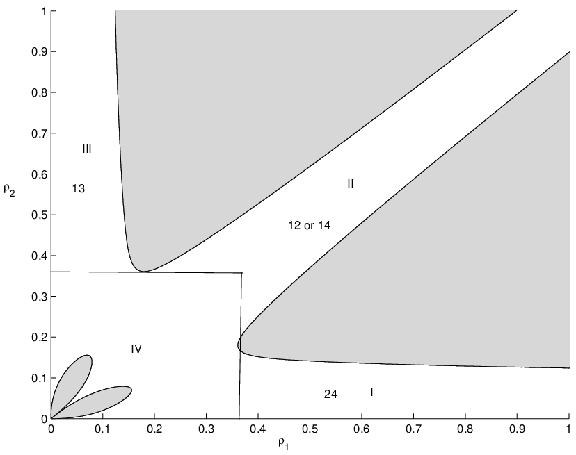
To monitor the hierarchies and its changes from one state to another we solve numerically equations (6.9) to (6.12) at any time to give the locations of the four bodies in the phase space with respect to each other. We will explain section 6.3 how we solve these equations. Once we find the position co-ordinates of all the four bodies, then it is not difficult to determine what hierarchy state the CS5BP system is in. See section 6.7 for the definition of hierarchy states for the CS5BP. To monitor the hierarchy changes during the integration time we make use of figure (6.2). Please note that figure (6.2) is different for each set of initial conditions. Region I and III represent single binary areas while region II represent double binary areas. If the system is in region I we say that it is in the 24 type of hierarchy state, if it is in region II we say that it is in the 12 or 14 hierarchy state depending on the distances and . If , then the system is in the 12 type of hierarchy state. Otherwise it is in the 14 type of hierarchy state. If the system is in region III then we say that it is in the 13 type of hierarchy state. But if the system is in region IV then we do not recognize any hierarchy state until it enters one of the other three regions. When the system transfers from one region to another, we record a hierarchy change. For example if the system goes out of region I and enters region IV and then region III we record this as a 24 13 (2313) hierarchy change and vice versa.
Note that this criterion for recognizing a hierarchy change is different from that of ?. Our criterion is based on the sizes of and relative to each other while Széll’s criterion is also based on changes from libration to rotation and vice versa of the angle between and . In practical terms, both methods produce similar frequencies of hierarchy type changes.
6.3 The Integrator
The equations of motion for the CS5BP, equations (6.9) to (6.12), are highly non-linear second order coupled differential equations. It is not possible to find their analytical solution. Therefore we have to use some numerical technique for integrating this system of the differential equation. The software must take as input data, the initial parameters of the differential equations and give as output data, the solution ( position and velocity coordinates) of differential equations belonging to the input data. To develop the integrator we first needed to find an accurate and fast numerical method and then develop an environment where the input and output data is efficiently handled.
The numerical method, we chose, for this integration project is a 15th order method with a adaptive step size control called the Radau method of Everhart [everhart]. This method makes use of Gauss-Radau spacing. We have adopted the FORTRAN code from the example of Everhart’s three body problem. We used Microsoft Visual C++ 6.0 to construct the environment of the integrator.
6.4 Initial Conditions
The numerical integrations of (6.9) to (6.12) require initial values for and . In order to satisfy the initial conditions of the CS5BP we immediately have
| (6.13) |
We choose a grid of values of and so that they range within the intervals (0, 3] and (0, 2.5], separated by an increment size 0.05. The initial velocities of and of are calculated using the following relations.
| (6.14) |
| (6.15) |
Where and are the components of and respectively, is the angular momentum of the system, is negative of the energy and is the potential given in chapter 4. The components of and are set to be zero for .
Our aim in this chapter is to examine the motion and stability of a variety of the CS5BP systems each with a different Szebehely constant . We also wish to compare systems with the same Szebehely constant. Thus we select the initial conditions so that they result in the same . For a given , the variables and can be calculated from equations (6.14) and (6.15).
We investigate the following sets of mass ratios of the CS5BP with several values of for each set of mass ratios. Diagram of the initial configuration for each set of mass ratios are given in table (6.1), along with section in which each system is discussed.
- 1.
The Four Body Cases i.e the CSFBP
- (a)
and , in CSFBP notation .
- (b)
, and , in CSFBP notation .
- (c)
, and , in CSFBP notation .
- (d)
, and , in CSFBP notation .
- (a)
- 2.
Equal mass case of the CS5BP i.e.
- 3.
Four equal masses with a varying central mass
- (a)
and ; Four equal masses with a very small central mass
- (b)
and ; Four equal masses with a comparatively larger central mass but still smaller than the outer bodies
- (c)
and ; Four equal masses with a large central mass and smaller outer bodies.
- (a)
- 4.
Three equal masses and two increasing symmetrically
- (a)
and
- (b)
and
- (c)
and
- (a)
- 5.
Non-equal masses
- (a)
, and
- (b)
, and
- (c)
, and
- (a)
The values of were chosen so as to represent each important region of the Szebehely ladder. Recall that , , and , the rungs of the Szebehely ladder, represent boundaries for at which topology of the phase space changes.
In order to analyze the behavior of the motion, for each case, approximately 3000 integrations were performed for over 1 million time-steps each. A total of 933000 = 279000 orbits were investigated numerically. Therefore the total integration time was well over 34 million time steps.
Initially the system is in the 12 (DB) or 24 (SB) hierarchy state when , see figure (7.3a), and it is in the 12 (DB) or 13 (SB) hierarchy state when , see figure (7.3b). Overall the CSFBP system is initially either in the 12 (DB), 13 (SB) or 24 (SB) hierarchy states. We do not initially place the system in a 14 hierarchy state, since it is equivalent to the 12 hierarchy state where only the numbering of the bodies differ. Both the cases 1) initially two larger masses in the centre and two smaller masses located outside ( ), and 2)two smaller masses in the centre and two larger masses located outside () are dealt with.
| Diagram | mass ratios | Section number |
| CSFBP | ||
| O–O––O–O | Section 7.5.1 | |
| O–O––O–O | ||
| o–O––O–o | ||
| o–O––O–o | ||
| Equal mass case of the CS5BP | ||
| O–O–O–O–O | Section 7.5.2 | |
| Four equal masses with a varying central mass | ||
| O–O–o–O–O | Section 7.5.3 | |
| O–O–O–O–O | ||
| o–o–O–o–o | ||
| Three equal masses and two increasing | ||
| symmetrically | ||
| O–O–O–O–O | Section 7.5.4 | |
| O–O–O–O–O | ||
| O–O–O–O–O | ||
| Non-equal masses | ||
| O–O–o–O–O | Section 7.5.5 | |
| O–o–o–o–O | ||
| O–o–O–o–O |
6.5 Hierarchical Stability of the CS5BP
We have given an analytical stability criterion for the CS5BP, in chapter 5, and we have shown that the CS5BP is hierarchically stable for . We have also shown that it is possible for the CS5BP to move from one hierarchy state to another for . We aim to understand the behavior of the CS5BP during the transition from the phase space being connected to it being disconnected.
To discuss the hierarchical stability of the CS5BP, we selected five values i.e. , , , and where is the critical value of denoted by for each mass ratio. The main reason for integrating for was to validate that the integrator was working properly and the numerical investigation agreed with the analytical prediction; i.e that the phase space is disconnected for and therefore the system is hierarchically stable.
For each set we integrated numerically approximately 3000 different orbits for about 1 million time steps of integration time. In order to study the hierarchical stability for each set we gathered data from the numerical integrations outputs on the number of hierarchy changes.
We have constructed two kinds of tables for each set, namely
- 1.
The frequency distribution of hierarchy changes: Columns represent fixed values while rows represent the number of each type of hierarchy changes. The number of hierarchy changes were calculated by determining the total number of hierarchy changes of each type which occurred throughout the many different integrations with the same set.
- 2.
Percentage of hierarchy changes: Columns represent fixed values while rows represent percentage of hierarchy changes.
Now we will discuss the hierarchical stability of the CS5BP for different mass ratios. First we will discuss the case which is a special case of the CS5BP called the CSFBP in the following section.
6.5.1 Hierarchical stability of the CSFBP, ( and )
In this section we will discuss the case of the CS5BP which is the CSFBP (Széll, 2003). Széll (2003) discussed a special case of the CSFBP for hierarchical stability. He discussed the case when or in other words when the larger masses were nearer to the centre of mass than the smaller masses, see figure (6.3a). Therefore he covered half of the phase space. He also always started in the 12, double binary, or the 24, single binary, hierarchy state or using the CSFBP notation the 12 or 23 hierarchy states. Recall that we have a difference of notation with ?, the CSFBP 13 (DB) hierarchy state is 14 (DB) and its 23 (SB) is 24 (SB) in our case and vice versa, for more details see section 6.1. We will use our notation in the whole thesis and whenever a comparison is necessary we will give the CSFBP notation in brackets as against to ours.

Our study of the case will complete Széll’s analysis of hierarchical stability of the CSFBP, as we will consider both and cases, see figure (6.3).
Equal mass case of the CSFBP (or in the CSFBP notation )
The critical values in this case are and . The results of integration are contained in Table (6.2).
There are no hierarchy changes for which confirm the analytical results we obtained in chapter 6. The most likely hierarchy changes for and are 12 24 and 12 13 and vice versa. The 12 24 hierarchy changes die out for higher values, while the 12 13 remain dominant. For higher values, the 13 12 hierarchy changes joins the race for the most likely hierarchy changes and remains considerably close to the 12 13 hierarchy changes. All of the above changes are from SB to DB and vice versa.
The most unlikely hierarchy changes are from double binary to double binary. These kind of hierarchy changes usually do not happen directly. There is usually a third kind of hierarchy change of intermediate hierarchy state which takes the system in to a new configuration. If we look at the average number of hierarchy changes from different hierarchy states we come to the conclusion that the 12 is the most unstable while 14 is comparatively more stable than all others. For example there are nearly twelve hundred hierarchy changes from the 12 hierarchy state to another, which is the most, and there are a little above five hundred from the 14 hierarchy state to another.
and or in CSFBP notation
The critical values in this case are . The total number of hierarchy changes of each for different values of are listed in Table (6.4). The corresponding percentages of different hierarchy changes are given in Table (6.5).
For the phase space is disconnected and therefore there are no hierarchy changes. At there are no hierarchy changes to or from the 24 hierarchy state which is exactly what the analytical stability criterion predicts i.e. there are no 12 24, 1424, 13 24, 24 12, 24 14 and 24 13 hierarchy changes.
The most likely hierarchy changes for small values are the 12 24. And the most unlikely hierarchy changes are the 24 14 and 14 24. Overall hierarchy changes from 14 to any other hierarchy state for all values are very small except for small values eg. where the 14 12 and 12 14 are the highest hierarchy changes. Hierarchy changes from double binary to double binary are very small as one would expect.
The main characteristics of this case is similar to those of the equal mass case. With small , we have more hierarchy changes and as increases the number of hierarchy changes decreases. The most unlikely hierarchy changes are still from double binary to double binary.
The main difference in this case and the equal mass case is that we have fewer hierarchy changes. Therefore the system is hierarchically more stable. Moreover in the equal mass case we were not able to identify any, comparatively, stable hierarchy states as all hierarchy states were equally unstable, but in this case we have some hierarchy states which can be considered hierarchically stable. For example Hierarchy changes from the 14 (DB) hierarchy state is approximately 1 percent, which is very nearly stable. As we decrease the value of we will be getting closer to a perturbed two+two body system and therefore we should expect a comparatively more stable situation.
and (or in CSFBP notation )
The critical values in this case are . The total number of hierarchy changes of each for different values of are listed in Table (6.6). The corresponding percentages of different hierarchy changes are given in Table (6.7).
There are no hierarchy changes with , since this value is greater than and therefore the phase space is disconnected.
At the Szebehely constant is a little less than and the phase space is partially disconnected. Therefore the hierarchy changes to or from the 24 hierarchy state are forbidden. In table (6.6) it can be seen that there are no 12 24, 14 24, 13 24, 24 12, 24 14 and 24 13 hierarchy changes, confirming numerically the analytical stability criterion.
As we were expecting from our experience of the previous , case the number of hierarchy changes decrease further as we decrease the value of . But the main characteristics remain the same. With small , 12 24, 24 12, and 13 24 hierarchy changes are dominant. This makes sense physically since as is increased, the situation of two large masses in the centre forming a single binary with two smaller masses orbiting their centre of mass (eg the 24 hierarchy) will begin to dominate the system. We can see this growing dominance of 24 hierarchies visually in the projection of allowed motion for this case figure (6.4) which shows an increased region of allowed motion. When is increased the number of hierarchy changes drop dramatically and the system is comparatively much more stable than the previous cases discussed so far. Again the most unlikely hierarchy changes are from double binary to double binary.
The main difference between the previous case and this case is that the system is hierarchically more stable as the system is now closer to the perturbed two+two body system.

and (or in CSFBP notation )
The critical values in this case are . The total number of hierarchy changes of each for different values of are listed in Table (6.8). The corresponding percentages of different hierarchy changes are given in Table (6.9).
There are only five hierarchy changes for the smallest value, which are the only hierarchy changes for the 15,000 orbits integrated for one million time steps of integration time. These few hierarchy changes are from 13 24, 24 13 and 24 12. The very small number of hierarchy changes indicate that the system is generally hierarchically stable. This is so because the system is close to a slightly perturbed two body system.
Comparison with Széll’s Analysis
To compare our analysis of the Caledonian Symmetric Problem (CSFBP) with Széll’s we have the following similarities and differences. Recall the difference in method of research with ? which might produce some differences.
- 1.
? counts for only half of the phase space (). This might produce a bias in favor of some hierarchy states.
- 2.
Our hierarchy changing criterion is different from ? as our criterion is based on the size of and relative to each other, while Széll’s criterion is also based on change from libration to rotation or vice versa of the angle between and .
? number and percent of hierarchy changes are tabulated in Appendix 1. Recall that when making comparisons you must take account of Széll’s different numbering of the four bodies from our numbering.
Differences
- 1.
For (or CSFBP notation ), the 12 24 and 24 12, (in CSFBP notation 12 and 23 12), hierarchy changes are much higher in our case than in Széll’s case. They are twenty percent to fourteen percent in our case and four percent to two percent in Széll’s case. See tables (6.2) and (6.3) and table 1 and 2 in appendix 1. These differences are most likely because of the inclusion of the second half of the phase space into our research which almost doubles the number of starting conditions for 12 hierarchy state. See appendix for ? results. When the value of increases, the hierarchy changes discussed above decrease in our case while it increases in Széll’s case.
- 2.
For all values of the Szebehely constant in the (or CSFBP notation ) case, the 12 24 (CSFBP notation 12 23)hierarchy changes are very high in our case while it is very small in Széll’s case. The 24 13 (CSFBP notation 23 14) hierarchy changes are very small in our case and stand at a maximum of nine percent. In Széll’s case they are very high and stands at thirty six percent maximum and ten percent minimum. See tables (6.4) and (6.5) and table 3 and 4 in appendix 1. These differences are also most likely because of the inclusion of the second half of the phase space. The size of the region of real motion in the non e-qual mass cases for the 13 (CSFBP notation 14) hierarchy state is very small therefore we have fewer starting conditions for this hierarchy state and thus we will have fewer hierarchy changes to or from this hierarchy state.
- 3.
For (or CSFBP notation ), the 13 24 hierarchy changes are very small (maximum fifteen percent) in our case and becomes zero near the critical value of the Szebehely constant which is the prediction of the analytical stability criterion. In Széll’s case these hierarchy changes are comparatively very high (maximum forty percent) and do not become zero near the critical value of the Szebehely constant which is against the prediction of the analytical stability criterion. See tables (6.6) and (6.7). Széll (2003) do not give any reason for this, see appendix for their results.
- 4.
For (0r CSFBP notation ), the 24 14 (CSFBP notation 23 13) hierarchy changes are zero in our case while it goes up to fifteen percent in Széll’s case.
- 5.
For (0r ), the 12 13 (CSFBP notation 12 14) and 12 24 (CSFBP notation 12 23) hierarchy changes are zero in our case while they are non-zero in Széll’s case and 12 13 (CSFBP notation 12 14) change increases from zero to thirty one percent when increases.
Similarities
- 1.
the main characteristics of both the analysis remain the same. The number of hierarchy changes decrease as the value of increases and the number of hierarchy changes are zero for
- 2.
- 3.
- 4.
For , in CSFBP notation ,the 14 24 (CSFBP: 13 23) hierarchy changes are the most unlikely in both cases.
- 5.
For , in CSFBP notation , the 13 24 (CSFBP: 14 23) and 24 13 (CSFBP: 23 14) hierarchy changes are the most likely in both the cases. Also the number of hierarchy changes are very small with 12 13, 14 12, 14 13 and 13 14 (CSFBP: 12 14, 13 12, 13 14, and 14 13) being zero.
| 12 13 | 179 | 143 | 150 | 125 | 104 | 0 |
|---|---|---|---|---|---|---|
| 12 14 | 5 | 0 | 10 | 22 | 12 | 0 |
| 12 24 | 204 | 162 | 24 | 33 | 11 | 0 |
| 13 12 | 91 | 9 | 141 | 119 | 90 | 0 |
| 13 14 | 66 | 10 | 21 | 20 | 28 | 0 |
| 13 24 | 56 | 18 | 28 | 27 | 20 | 0 |
| 14 12 | 5 | 0 | 11 | 13 | 19 | 0 |
| 14 13 | 60 | 32 | 24 | 41 | 38 | 0 |
| 14 24 | 80 | 84 | 36 | 37 | 26 | 0 |
| 24 12 | 146 | 130 | 32 | 33 | 21 | 0 |
| 24 13 | 130 | 90 | 32 | 33 | 41 | 0 |
| 24 14 | 85 | 74 | 26 | 25 | 26 | 0 |
| Total | 1022 | 678 | 509 | 503 | 410 | 0 |
| 12 13 | 17.51 | 21.09 | 22.12 | 18.44 | 15.34 | 0 |
| 12 14 | 0.49 | 0 | 1.47 | 3.24 | 1.77 | 0 |
| 12 24 | 19.96 | 24.89 | 3.54 | 4.87 | 1.62 | 0 |
| 13 12 | 8.9 | 1.33 | 20.8 | 17.55 | 13.27 | 0 |
| 13 14 | 6.46 | 1.47 | 3.1 | 2.95 | 4.13 | 0 |
| 13 24 | 5.48 | 2.65 | 4.13 | 3.98 | 2.95 | 0 |
| 14 12 | 0.49 | 0 | 1.62 | 1.92 | 2.8 | 0 |
| 14 13 | 5.87 | 4.72 | 3.54 | 6.05 | 5.6 | 0 |
| 14 24 | 7.83 | 12.39 | 5.31 | 5.46 | 3.83 | 0 |
| 24 12 | 14.29 | 19.17 | 4.72 | 4.87 | 3.1 | 0 |
| 24 13 | 12.72 | 13.27 | 4.72 | 4.87 | 6.05 | 0 |
| 24 14 | 8.32 | 10.91 | 3.83 | 3.69 | 3.83 | 0 |
| 12 13 | 132 | 98 | 121 | 9 | 0 |
|---|---|---|---|---|---|
| 12 14 | 1 | 5 | 5 | 16 | 0 |
| 12 24 | 360 | 348 | 90 | 0 | 0 |
| 13 12 | 55 | 61 | 73 | 2 | 0 |
| 13 14 | 2 | 5 | 3 | 0 | 0 |
| 13 24 | 136 | 138 | 46 | 0 | 0 |
| 14 12 | 5 | 11 | 3 | 16 | 0 |
| 14 13 | 5 | 8 | 6 | 0 | 0 |
| 14 24 | 0 | 2 | 2 | 0 | 0 |
| 24 12 | 78 | 57 | 22 | 0 | 0 |
| 24 13 | 77 | 56 | 22 | 0 | 0 |
| 24 14 | 0 | 3 | 1 | 0 | 0 |
| Total | 851 | 792 | 394 | 43 | 0 |
| 12 13 | 16 | 12 | 31 | 21 | 0 |
|---|---|---|---|---|---|
| 12 14 | 0 | 1 | 1 | 37 | 0 |
| 12 24 | 42 | 44 | 24 | 0 | 0 |
| 13 12 | 6 | 8 | 19 | 5 | 0 |
| 13 14 | 0 | 1 | 1 | 0 | 0 |
| 13 24 | 16 | 17 | 12 | 0 | 0 |
| 14 12 | 1 | 1 | 1 | 37 | 0 |
| 14 13 | 1 | 1 | 2 | 0 | 0 |
| 14 24 | 0 | 0 | 1 | 0 | 0 |
| 24 12 | 9 | 7 | 6 | 0 | 0 |
| 24 13 | 9 | 7 | 6 | 0 | 0 |
| 24 14 | 0 | 0 | 0 | 0 | 0 |
| 12 13 | 41 | 17 | 4 | 8 | 0 |
|---|---|---|---|---|---|
| 12 14 | 15 | 0 | 0 | 0 | 0 |
| 12 24 | 78 | 3 | 2 | 0 | 0 |
| 13 12 | 19 | 5 | 4 | 4 | 0 |
| 13 14 | 2 | 0 | 0 | 0 | 0 |
| 13 24 | 46 | 1 | 3 | 0 | 0 |
| 14 12 | 9 | 0 | 0 | 0 | 0 |
| 14 13 | 12 | 0 | 0 | 0 | 0 |
| 14 24 | 0 | 0 | 0 | 0 | 0 |
| 24 12 | 47 | 0 | 2 | 0 | 0 |
| 24 13 | 37 | 0 | 4 | 0 | 0 |
| 24 14 | 0 | 0 | 0 | 0 | 0 |
| Total | 306 | 27 | 19 | 12 | 0 |
| 12 13 | 13 | 63 | 21 | 67 | 0 |
|---|---|---|---|---|---|
| 12 14 | 5 | 0 | 0 | 0 | 0 |
| 12 24 | 25 | 11 | 11 | 0 | 0 |
| 13 12 | 6 | 19 | 21 | 33 | 0 |
| 13 14 | 1 | 0 | 0 | 0 | 0 |
| 13 24 | 15 | 4 | 16 | 0 | 0 |
| 14 12 | 3 | 0 | 0 | 0 | 0 |
| 14 13 | 4 | 0 | 0 | 0 | 0 |
| 14 24 | 0 | 0 | 0 | 0 | 0 |
| 24 12 | 15 | 4 | 11 | 0 | 0 |
| 24 13 | 12 | 0 | 21 | 0 | 0 |
| 24 14 | 0 | 0 | 0 | 0 | 0 |
| 12 13 | 0 | 0 | 0 | 0 | 0 |
|---|---|---|---|---|---|
| 12 14 | 0 | 0 | 0 | 0 | 0 |
| 12 24 | 0 | 0 | 0 | 0 | 0 |
| 13 12 | 0 | 0 | 0 | 0 | 0 |
| 13 14 | 0 | 0 | 0 | 0 | 0 |
| 13 24 | 2 | 0 | 0 | 0 | 0 |
| 14 12 | 0 | 0 | 0 | 0 | 0 |
| 14 13 | 0 | 0 | 0 | 0 | 0 |
| 14 24 | 0 | 0 | 0 | 0 | 0 |
| 24 12 | 1 | 0 | 0 | 0 | 0 |
| 24 13 | 2 | 0 | 0 | 0 | 0 |
| 24 14 | 0 | 0 | 0 | 0 | 0 |
| Total | 5 | 0 | 0 | 0 | 0 |
| 12 13 | 0 | 0 | 0 | 0 | 0 |
|---|---|---|---|---|---|
| 12 14 | 0 | 0 | 0 | 0 | 0 |
| 12 24 | 0 | 0 | 0 | 0 | 0 |
| 13 12 | 0 | 0 | 0 | 0 | 0 |
| 13 14 | 0 | 0 | 0 | 0 | 0 |
| 13 24 | 40 | 0 | 0 | 0 | 0 |
| 14 12 | 0 | 0 | 0 | 0 | 0 |
| 14 13 | 0 | 0 | 0 | 0 | 0 |
| 14 24 | 0 | 0 | 0 | 0 | 0 |
| 24 12 | 20 | 0 | 0 | 0 | 0 |
| 24 13 | 40 | 0 | 0 | 0 | 0 |
| 24 14 | 0 | 0 | 0 | 0 | 0 |
6.5.2 Equal mass case of the CS5BP,
The critical values in this case are and . The results are contained in Table (6.10).
There are no hierarchy changes for which is also the prediction of the analytical criterion. The most likely hierarchy changes for are the 14 24 and 24 14. When we increase the value of to 0.06 the 12 14 changes become the most likely hierarchy change which is from double binary to double binary. The most unlikely hierarchy changes are for all the values are those involving changes to and from 13.
The main characteristic of this case is similar to that of the CSFBP i.e. the number of hierarchy changes decreases as the value of increases; however there are some differences as follows.
- 1.
There are fewer hierarchy changes overall than for the equal mass case of the CSFBP which means that the extra central mass has played a stabilizing role in terms of hierarchical stability and therefore the equal mass CS5BP is more stable than the equal mass CSFBP.
- 2.
| 12 13 | 14 | 0 | 0 |
|---|---|---|---|
| 12 14 | 54 | 50 | 0 |
| 12 24 | 19 | 10 | 0 |
| 13 12 | 8 | 2 | 0 |
| 13 14 | 18 | 6 | 0 |
| 13 24 | 10 | 1 | 0 |
| 14 12 | 16 | 9 | 0 |
| 14 13 | 17 | 11 | 0 |
| 14 24 | 83 | 15 | 0 |
| 24 12 | 18 | 20 | 0 |
| 24 13 | 15 | 7 | 0 |
| 24 14 | 67 | 10 | 0 |
| Total | 339 | 141 | 0 |
| 12 13 | 4 | 0 | 0 |
|---|---|---|---|
| 12 14 | 16 | 36 | 0 |
| 12 24 | 6 | 7 | 0 |
| 13 12 | 2 | 1 | 0 |
| 13 14 | 5 | 4 | 0 |
| 13 24 | 3 | 1 | 0 |
| 14 12 | 5 | 6 | 0 |
| 14 13 | 5 | 8 | 0 |
| 14 24 | 24 | 11 | 0 |
| 24 12 | 5 | 14 | 0 |
| 24 13 | 4 | 5 | 0 |
| 24 14 | 20 | 7 | 0 |
6.5.3 Four equal masses with a varying central mass
In this section we introduce a stationary mass to the centre of the equal mass CSFBP and will use it to discover the effect of changing its mass on the hierarchical stability of the system. First we place a small mass at the centre of mass and then we increase it until the mass of the central body is much higher than the outer bodies. We discuss the following three different sets of mass ratios:
- 1.
and : Four equal masses with a very small central mass;
- 2.
and : Four equal masses with a comparatively larger central mass but still smaller than the outer bodies;
- 3.
and : Four equal masses with a large central mass and small outer bodies.
Four equal masses with a very small central mass ( and )
There are no hierarchy changes for which is also the prediction of the analytical stability criterion. The most likely hierarchy changes for small are 12 13 and 13 12. We have seen in the equal mass CS5BP that the single binary to double binary hierarchy changes and vice versa were small FOR large . These have increased after reducing the size of the central mass with in particular to and from 13 changes become larger.
The main difference between this case and the equal mass CSFBP is that we have fewer hierarchy changes. Compared to the equal mass CS5BP, this case has more hierarchy changes. An increasing central mass appears to stabilize the system. We shall see this confirmed in the next two sections.
Four equal masses with a slightly bigger central mass ( and )
We have increased the mass of the central body further but is still smaller than the four outer bodies. The total number of hierarchy changes decreased further but are still more than we had in the equal mass case of the CS5BP. The introduction of the central mass is indeed playing a stabilizing role. The most likely hierarchy changes in this case are 14 24 which were the most unlikely in the previous case with a smaller central mass. The most unlikely hierarchy changes are from 13 to any other hierarchy state for .
The main characteristic of both the cases remain the same. There are no hierarchy changes for and the number of hierarchies decreases as the value of the Szebehely constant increases.
Four equal masses with a very large central mass ( and )
We have further increased the mass of the central body so that the central body is 96 times bigger than the outer bodies i.e. . This system is close to a planetary system with a star in the centre with four planets.
The total number of hierarchy changes does not decrease much and is almost the same as we had in the previous case suggesting a similar level of instability. This is deceiving if we do not look at the individual members of the table. Most of the hierarchy changes are coming from 14 24 and vice versa. For small (), 14 24 and 24 14 changes contribute 74 percent to the total number of hierarchy changes and for large (), they contribute more than 99.9 percent of the total hierarchy changes. See tables (6.16) and (6.17).
There are no hierarchy changes from 12 13, 12 14, 13 12, 14 12 and 14 13 throughout the integrations carried out for this case. This system is comparatively much more stable than any other case of four equal masses with or without a stationary central mass.
As we have seen from all other cases of four equal masses with a stationary central mass and without a stationary central mass, the number of hierarchy changes decreases as the central mass increases. In the equal mass case of the CSFBP with no central mass the number of hierarchy changes were highest then after the introduction of the central mass the number of hierarchy changes decreased as we increased the central mass. Therefore now we can conjecture that the larger the central mass the more stable the system becomes.
| 12 13 | 96 | 60 | 0 |
|---|---|---|---|
| 12 14 | 30 | 12 | 0 |
| 12 24 | 22 | 20 | 0 |
| 13 12 | 83 | 65 | 0 |
| 13 14 | 31 | 25 | 0 |
| 13 24 | 26 | 10 | 0 |
| 14 12 | 44 | 31 | 0 |
| 14 13 | 63 | 51 | 0 |
| 14 24 | 26 | 5 | 0 |
| 24 12 | 28 | 15 | 0 |
| 24 13 | 39 | 40 | 0 |
| 24 14 | 19 | 8 | 0 |
| Total | 507 | 342 | 0 |
| 12 13 | 19 | 18 | 0 |
|---|---|---|---|
| 12 14 | 6 | 4 | 0 |
| 12 24 | 4 | 6 | 0 |
| 13 12 | 16 | 19 | 0 |
| 13 14 | 6 | 7 | 0 |
| 13 24 | 5 | 3 | 0 |
| 14 12 | 9 | 9 | 0 |
| 14 13 | 12 | 15 | 0 |
| 14 24 | 5 | 1 | 0 |
| 24 12 | 6 | 4 | 0 |
| 24 13 | 8 | 12 | 0 |
| 24 14 | 4 | 2 | 0 |
| 12 13 | 45 | 4 | 0 |
|---|---|---|---|
| 12 14 | 35 | 27 | 0 |
| 12 24 | 29 | 19 | 0 |
| 13 12 | 22 | 2 | 0 |
| 13 14 | 22 | 10 | 0 |
| 13 24 | 22 | 15 | 0 |
| 14 12 | 30 | 20 | 0 |
| 14 13 | 32 | 25 | 0 |
| 14 24 | 93 | 37 | 0 |
| 24 12 | 34 | 14 | 0 |
| 24 13 | 24 | 12 | 0 |
| 24 14 | 75 | 29 | 0 |
| Total | 462 | 214 | 0 |
| 12 13 | 10 | 2 | 0 |
|---|---|---|---|
| 12 14 | 8 | 13 | 0 |
| 12 24 | 6 | 9 | 0 |
| 13 12 | 5 | 1 | 0 |
| 13 14 | 5 | 5 | 0 |
| 13 24 | 5 | 7 | 0 |
| 14 12 | 6 | 9 | 0 |
| 14 13 | 7 | 12 | 0 |
| 14 24 | 20 | 17 | 0 |
| 24 12 | 7 | 7 | 0 |
| 24 13 | 5 | 6 | 0 |
| 24 14 | 16 | 14 | 0 |
| 12 13 | 0 | 0 | 0 |
|---|---|---|---|
| 12 14 | 0 | 0 | 0 |
| 12 24 | 32 | 0 | 0 |
| 13 12 | 0 | 0 | 0 |
| 13 14 | 1 | 0 | 0 |
| 13 24 | 26 | 0 | 0 |
| 14 12 | 0 | 0 | 0 |
| 14 13 | 0 | 1 | 0 |
| 14 24 | 136 | 52 | 0 |
| 24 12 | 32 | 0 | 0 |
| 24 13 | 27 | 0 | 0 |
| 24 14 | 196 | 93 | 0 |
| Total | 450 | 146 | 0 |
| 12 13 | 0 | 0 | 0 |
|---|---|---|---|
| 12 14 | 0 | 0 | 0 |
| 12 24 | 7 | 0 | 0 |
| 13 12 | 0 | 0 | 0 |
| 13 14 | 0 | 0 | 0 |
| 13 24 | 6 | 0 | 0 |
| 14 12 | 0 | 0 | 0 |
| 14 13 | 0 | 1 | 0 |
| 14 24 | 30 | 36 | 0 |
| 24 12 | 7 | 0 | 0 |
| 24 13 | 6 | 0 | 0 |
| 24 14 | 44 | 64 | 0 |
6.5.4 Three equal masses and two increasing symmetrically
In this section we will discuss a new case of the Caledonian Symmetric Five Body Problem. This is a completely different situation from those discussed earlier and little comparison with the previous cases will be made. Here we take the masses of three of the bodies to be equal and two of them to be varying symmetrically from being very small to very large and effectively approaching a situation of a perturbed two body problem. The three bodies with equal masses will comprise of two outer bodies and the central body i.e. . will increase to the largest masses from being the smallest. We will discuss the following three cases.
- 1.
and
- 2.
and
- 3.
and
and
There are no hierarchy changes for . Since this value is greater than the critical value, this fact shows that the numerical integrations follow well the analytical stability criterion.
The most unlikely hierarchy changes are 14 24. The 12 13, 13 12, 13 24, 24 13 and 24 14 hierarchy changes are also very small for small (). The 14 24 and 13 24 hierarchy changes remains the smallest for all values of .
For small , 12 14 and 14 12 hierarchy changes are the most likely and remain amongst the highest throughout the integrations carried out for this case of the CS5BP. These hierarchy changes remain the highest throughout the integration.
At the Szebehely constant is near and the phase space is partially disconnected. Therefore the hierarchy changes to or from the 13 hierarchy state are not allowed. This is numerically confirmed in table (6.16) where there are no 12 13, 13 12, 13 14, 13 24, 14 13 and 24 13 hierarchy changes.
The main characteristic of this case is similar to all other cases of the CS5BP. With small we have more hierarchy changes and as increases the number of hierarchy changes decrease.
and
In this case we increase the value of to 0.275 and consequently the value of decreases and hence we have .
There are no hierarchy changes for . For which is near the critical value there are no hierarchy changes from and to the 24 hierarchy state which is also the prediction of analytical stability criterion. The most likely hierarchy changes for small () are 14 24 and 12 24. When increases the 14 24 hierarchy changes decrease and the 12 24 changes remains the most likely until it dies out for large (). The most unlikely hierarchy changes are 12 14 and 13 14.
The main characteristic of this case and all other cases remain the same i.e. the number of hierarchy changes decreases as increases.
and
The critical values in this case are . Results are contained in tables (6.22) and (7.23).
In this case we further decrease the value of and and consequently the value of increases. As therefore this can be considered a perturbed two body problem.
There are no hierarchy changes for any value of we have investigated. See table (6.22). We have investigated about 15,000 orbits each for 1 million time steps of integration time and there are no hierarchy changes. Therefore this is the most stable of the CS5BP systems we have discussed so far in this chapter.
| 12 13 | 15 | 7 | 11 | 0 | 0 |
|---|---|---|---|---|---|
| 12 14 | 108 | 24 | 21 | 15 | 0 |
| 12 24 | 45 | 26 | 24 | 15 | 0 |
| 13 12 | 22 | 6 | 6 | 0 | 0 |
| 13 14 | 78 | 7 | 10 | 0 | 0 |
| 13 24 | 11 | 3 | 3 | 0 | 0 |
| 14 12 | 103 | 24 | 28 | 21 | 0 |
| 14 13 | 84 | 7 | 3 | 0 | 0 |
| 14 24 | 6 | 2 | 1 | 1 | 0 |
| 24 12 | 35 | 14 | 8 | 4 | 0 |
| 24 13 | 15 | 6 | 8 | 0 | 0 |
| 24 14 | 14 | 5 | 5 | 7 | 0 |
| Total | 536 | 130 | 128 | 63 | 0 |
| 12 13 | 3 | 5 | 9 | 0 | 0 |
|---|---|---|---|---|---|
| 12 14 | 20 | 18 | 16 | 24 | 0 |
| 12 24 | 8 | 20 | 19 | 24 | 0 |
| 13 12 | 4 | 5 | 5 | 0 | 0 |
| 13 14 | 15 | 5 | 8 | 0 | 0 |
| 13 24 | 2 | 2 | 2 | 0 | 0 |
| 14 12 | 19 | 18 | 22 | 33 | 0 |
| 14 13 | 16 | 5 | 2 | 0 | 0 |
| 14 24 | 1 | 2 | 1 | 2 | 0 |
| 24 12 | 7 | 11 | 6 | 6 | 0 |
| 24 13 | 3 | 5 | 6 | 0 | 0 |
| 24 14 | 3 | 4 | 4 | 11 | 0 |
| 12 13 | 38 | 24 | 16 | 0 | 0 |
|---|---|---|---|---|---|
| 12 14 | 26 | 13 | 74 | 14 | 0 |
| 12 24 | 67 | 70 | 99 | 0 | 0 |
| 13 12 | 20 | 20 | 8 | 0 | 0 |
| 13 14 | 14 | 7 | 38 | 3 | 0 |
| 13 24 | 47 | 26 | 27 | 0 | 0 |
| 14 12 | 24 | 17 | 72 | 22 | 0 |
| 14 13 | 30 | 18 | 36 | 4 | 0 |
| 14 24 | 86 | 42 | 16 | 0 | 0 |
| 24 12 | 53 | 28 | 37 | 0 | 0 |
| 24 13 | 44 | 17 | 34 | 0 | 0 |
| 24 14 | 47 | 35 | 24 | 0 | 0 |
| Total | 496 | 317 | 480 | 43 | 0 |
| 12 13 | 8 | 8 | 3 | 0 | 0 |
|---|---|---|---|---|---|
| 12 14 | 5 | 4 | 15 | 33 | 0 |
| 12 24 | 14 | 22 | 21 | 0 | 0 |
| 13 12 | 4 | 6 | 2 | 0 | 0 |
| 13 14 | 3 | 2 | 8 | 7 | 0 |
| 13 24 | 9 | 8 | 6 | 0 | 0 |
| 14 12 | 5 | 5 | 15 | 51 | 0 |
| 14 13 | 6 | 6 | 8 | 9 | 0 |
| 14 24 | 17 | 13 | 3 | 0 | 0 |
| 24 12 | 11 | 9 | 8 | 0 | 0 |
| 24 13 | 9 | 5 | 7 | 0 | 0 |
| 24 14 | 9 | 11 | 5 | 0 | 0 |
| 12 13 | 0 | 0 | 0 | 0 | 0 |
|---|---|---|---|---|---|
| 12 14 | 0 | 0 | 0 | 0 | 0 |
| 12 24 | 0 | 0 | 0 | 0 | 0 |
| 13 12 | 0 | 0 | 0 | 0 | 0 |
| 13 14 | 0 | 0 | 0 | 0 | 0 |
| 13 24 | 0 | 0 | 0 | 0 | 0 |
| 14 12 | 0 | 0 | 0 | 0 | 0 |
| 14 13 | 0 | 0 | 0 | 0 | 0 |
| 14 24 | 0 | 0 | 0 | 0 | 0 |
| 24 12 | 0 | 0 | 0 | 0 | 0 |
| 24 13 | 0 | 0 | 0 | 0 | 0 |
| 24 14 | 0 | 0 | 0 | 0 | 0 |
| Total | 0 | 0 | 0 | 0 | 0 |
| 12 13 | 0 | 0 | 0 | 0 | 0 |
|---|---|---|---|---|---|
| 12 14 | 0 | 0 | 0 | 0 | 0 |
| 12 24 | 0 | 0 | 0 | 0 | 0 |
| 13 12 | 0 | 0 | 0 | 0 | 0 |
| 13 14 | 0 | 0 | 0 | 0 | 0 |
| 13 24 | 0 | 0 | 0 | 0 | 0 |
| 14 12 | 0 | 0 | 0 | 0 | 0 |
| 14 13 | 0 | 0 | 0 | 0 | 0 |
| 14 24 | 0 | 0 | 0 | 0 | 0 |
| 24 12 | 0 | 0 | 0 | 0 | 0 |
| 24 13 | 0 | 0 | 0 | 0 | 0 |
| 24 14 | 0 | 0 | 0 | 0 | 0 |
6.5.5 Non-Equal mass cases of the CS5BP
The cases of the CS5BP we have discussed so far had at least two or more of the mass ratios equal which included, and , , and , and and . In this section we discuss the cases of the CS5BP where none of the mass ratios are equal. We will discuss the following three sets of mass ratios:
- 1.
, and
- 2.
, and
- 3.
, and
, and
There are no hierarchy changes for as was predicted by the analytical stability criterion. For there are no hierarchy changes to or from the 24 hierarchy state which is exactly what the analytical stability criterion predicts.
The most likely hierarchy changes are always to or from the 24 hierarchy state until it becomes disconnected from all other hierarchy states. For small (), the 24 13 hierarchy changes are the highest, for , the 13 24 hierarchy changes is the highest and for large (), the 24 13 hierarchy changes are again the highest which means that the 24 hierarchy state is the most unstable for small values of the Szebehely constant, . Also the most number of hierarchy changes are from the 24 hierarchy state which is another reason for branding the 24 hierarchy state the most unstable for small .
The most unlikely hierarchy changes are from the 14 hierarchy state for and 0.04. This suggests that the 14 hierarchy state is the most stable hierarchy state but perhaps it is the result of not starting in the 14 hierarchy state. Fewer starts in the 14 hierarchy mean fewer changes from it are possible. At large, , the 14 hierarchy state appears to be contributing more than 50 percent to the total hierarchy changes and turns out to be unstable. For large values of the Szebehely constant near the critical value the 24 hierarchy state is the most stable opposite to the fact that it is the most unstable situation for small .
The main characteristic of this case and all other cases of the CS5BP discussed so far remain the same. There are no hierarchy changes for and the number of hierarchy changes decrease as the value of increases. There is a sudden decrease in the total number of hierarchy changes near but this is not unexpected as at this point the 24 hierarchy state which was the main contributor disconnects and therefore the total number of hierarchy changes drop.
, and
We increase the value of from 0.01 to 0.2 from the last case and the total number of hierarchy changes drop dramatically. As we said earlier, the bigger the central mass, the more stable the system would be and this behavior compliments our statement.
There are no hierarchy changes for . For large, the number of hierarchy changes are zero which is another reason to believe that this system is comparatively more stable than the , and case discussed earlier. The number of hierarchy changes from the 14 hierarchy state are very small throughout the integrations performed for this set of mass ratios and becomes zero for and therefore 14 is the most stable hierarchy state. Recall that 14 was the most stable hierarchy state in the previous case too. The 24 12 and 24 13 hierarchy changes are also very small and is the most unlikely for and . See table (6.26).
The most likely hierarchy changes for and are 12 13. For the highest number of hierarchy changes are from 13 to 24. See table (6.26).
, and
The total number of hierarchy changes further dropped as the value of increased and decreased. There are no hierarchy changes for and . There are no hierarchy changes from the 14 hierarchy state except one 14 24 hierarchy changes for , see table (6.28). Therefore the 14 hierarchy state continue to be the most stable for all the three sets of mass ratios discussed in this section. There are also no 12 14 and 14 12 hierarchy changes which is the double binary to double binary. For this particular set of mass ratios the double binary hierarchy states i.e. 12 and 14 appear to be more stable as there are very few hierarchy changes from 12 as well.
The most likely hierarchy changes are to or from the 24 hierarchy state as the size of the region of real motion is larger than the others for 24 hierarchy state. The 24 13 and the 13 24 hierarchy changes are the highest for and for . For the 24 12 and 12 24 hierarchy changes are the highest.
It is very interesting to see that in all the three sets of mass ratios discussed in this section, the 14 hierarchy state which is a double binary was the most stable and the 24 hierarchy state, which a single binary, was the most unstable.
The main characteristic of all the cases of the CS5BP discussed in this chapter remains the same. There are no hierarchy changes for the Szebehely constant greater than the critical value and the number of hierarchy changes decreases as is increased.
| 12 13 | 58 | 50 | 56 | 14 | 0 |
|---|---|---|---|---|---|
| 12 14 | 14 | 7 | 22 | 12 | 0 |
| 12 24 | 48 | 40 | 50 | 0 | 0 |
| 13 12 | 56 | 34 | 21 | 2 | 0 |
| 13 14 | 9 | 7 | 6 | 0 | 0 |
| 13 24 | 38 | 67 | 17 | 0 | 0 |
| 14 12 | 10 | 12 | 14 | 20 | 0 |
| 14 13 | 16 | 12 | 9 | 10 | 0 |
| 14 24 | 6 | 9 | 0 | 0 | 0 |
| 24 12 | 85 | 53 | 33 | 0 | 0 |
| 24 13 | 93 | 60 | 49 | 0 | 0 |
| 24 14 | 9 | 5 | 0 | 0 | 0 |
| Total | 442 | 356 | 277 | 58 | 0 |
| 12 13 | 13 | 14 | 20 | 24 | 0 |
|---|---|---|---|---|---|
| 12 14 | 3 | 2 | 8 | 21 | 0 |
| 12 24 | 11 | 11 | 18 | 0 | 0 |
| 13 12 | 13 | 10 | 8 | 3 | 0 |
| 13 14 | 2 | 2 | 2 | 0 | 0 |
| 13 24 | 9 | 19 | 6 | 0 | 0 |
| 14 12 | 2 | 3 | 5 | 34 | 0 |
| 14 13 | 4 | 3 | 3 | 17 | 0 |
| 14 24 | 1 | 3 | 0 | 0 | 0 |
| 24 12 | 19 | 15 | 12 | 0 | 0 |
| 24 13 | 21 | 17 | 18 | 0 | 0 |
| 24 14 | 2 | 1 | 0 | 0 | 0 |
| 12 13 | 84 | 55 | 1 | 0 | 0 |
|---|---|---|---|---|---|
| 12 14 | 16 | 16 | 4 | 0 | 0 |
| 12 24 | 12 | 18 | 18 | 0 | 0 |
| 13 12 | 26 | 12 | 5 | 0 | 0 |
| 13 14 | 19 | 19 | 0 | 0 | 0 |
| 13 24 | 4 | 10 | 30 | 0 | 0 |
| 14 12 | 9 | 6 | 0 | 0 | 0 |
| 14 13 | 19 | 19 | 0 | 0 | 0 |
| 14 24 | 19 | 28 | 0 | 0 | 0 |
| 24 12 | 8 | 5 | 6 | 0 | 0 |
| 24 13 | 8 | 13 | 5 | 0 | 0 |
| 24 14 | 26 | 35 | 0 | 0 | 0 |
| Total | 250 | 246 | 69 | 0 | 0 |
| 12 13 | 34 | 24 | 1 | 0 | 0 |
|---|---|---|---|---|---|
| 12 14 | 6 | 7 | 6 | 0 | 0 |
| 12 24 | 5 | 8 | 26 | 0 | 0 |
| 13 12 | 10 | 5 | 7 | 0 | 0 |
| 13 14 | 8 | 8 | 0 | 0 | 0 |
| 13 24 | 2 | 4 | 43 | 0 | 0 |
| 14 12 | 4 | 3 | 0 | 0 | 0 |
| 14 13 | 8 | 8 | 0 | 0 | 0 |
| 14 24 | 8 | 12 | 0 | 0 | 0 |
| 24 12 | 3 | 2 | 9 | 0 | 0 |
| 24 13 | 3 | 6 | 7 | 0 | 0 |
| 24 14 | 10 | 15 | 0 | 0 | 0 |
| 12 13 | 0 | 3 | 0 | 0 | 0 |
|---|---|---|---|---|---|
| 12 14 | 0 | 0 | 0 | 0 | 0 |
| 12 24 | 8 | 6 | 2 | 0 | 0 |
| 13 12 | 0 | 3 | 0 | 0 | 0 |
| 13 14 | 0 | 0 | 0 | 0 | 0 |
| 13 24 | 17 | 3 | 0 | 0 | 0 |
| 14 12 | 0 | 0 | 0 | 0 | 0 |
| 14 13 | 0 | 0 | 0 | 0 | 0 |
| 14 24 | 0 | 0 | 1 | 0 | 0 |
| 24 12 | 14 | 6 | 1 | 0 | 0 |
| 24 13 | 17 | 4 | 0 | 0 | 0 |
| 24 14 | 2 | 0 | 1 | 0 | 0 |
| Total | 58 | 25 | 5 | 0 | 0 |
| 12 13 | 0 | 12 | 0 | 0 | 0 |
|---|---|---|---|---|---|
| 12 14 | 0 | 0 | 0 | 0 | 0 |
| 12 24 | 14 | 24 | 40 | 0 | 0 |
| 13 12 | 0 | 12 | 0 | 0 | 0 |
| 13 14 | 0 | 0 | 0 | 0 | 0 |
| 13 24 | 29 | 12 | 0 | 0 | 0 |
| 14 12 | 0 | 0 | 0 | 0 | 0 |
| 14 13 | 0 | 0 | 0 | 0 | 0 |
| 14 24 | 0 | 0 | 20 | 0 | 0 |
| 24 12 | 24 | 24 | 20 | 0 | 0 |
| 24 13 | 29 | 16 | 0 | 0 | 0 |
| 24 14 | 3 | 0 | 20 | 0 | 0 |
6.6 Conclusions
The numerical investigations shows that the introduction of a small stationary mass to the centre of mass of the Caledonian Symmetric Four Body Problem (CSFBP) plays a stabilizing role. The number of hierarchy changes decreases as we increase the value of i.e. the central mass. This can be applied to a system of four planets and one star at the centre of mass of the system. We have seen that such system is hierarchically stable, see for example the analysis and tables provided for and .
The numerical investigations support the analytical predictions i.e. that the phase space is disconnected for . In some cases the analytical curves predicted that the phase space is partially disconnected eg. for . This is also supported by the numerical investigations.
The stability of the four and five body systems increases as the value of or decreases. With small or the system is close to a three body system perturbed by two bodies of negligible mass. In the case of or very small as compared to the other mass ratio then, the system is close to a perturbed two body system.
Numerical investigations of all the CS5BP systems discussed in this chapter reveal that as the value of the Szebehely constant increases the number of hierarchy changes decreases and hence their hierarchical stability improves. Therefore it can be stated for the Szebehely constant near zero the system will be very unstable, for increasing it will become more stable and for greater than the critical value it will be hierarchically stable for all time.
We have seen that the studies of the CSFBP and the CS5BP have given valuable information to understand better the general problems. Therefore it is of interest to generalize the CS5BP system in the next chapter for any number of bodies.
Chapter 7 The Caledonian Symmetric N Body Problem
In chapter 5 we investigated the Caledonian Symmetric five Body Problem (CS5BP), which is a symmetrically reduced five body problem containing all possible symmetries in the phase space. We have found an analytical stability criterion for the CS5BP. In chapter 5 we numerically verified this stability criterion and have shown that , the Szebehely constant, plays a very important role in determining the hierarchical stability criterion of the CS5BP.
In this chapter we generalize the CS5BP to the CSNBP i.e the Caledonian Symmetric N Body Problem in such a way that it can be easily used for any number of bodies such as three, four (CSFBP) and five (CS5BP) etc. In section 7.1 we define the CSNBP. The equations of motion and Sundman’s inequality, the key to the stability criterion, are given in sections 7.2 and 7.3 respectively. We then derive in sections 7.4 and 7.5 the analytical stability criterion for the CSNBP. The conclusions are given in section 7.6.
7.1 Definition of the Caledonian Symmetric N Body Problem (CSNBP)
The CSNBP is formulated by using all possible symmetries. The main feature of the model is its use of two types of symmetries. 1. past-future symmetry and 2. dynamical symmetry. Past future symmetry exists in an n-body system when the dynamical evolution of the system after is a mirror image of the dynamical evolution of the system before . It occurs whenever the system passes through a mirror configuration, a configuration in which the velocity vectors of all the bodies are perpendicular to all the position vectors from the centre of mass of the system (Roy and Ovenden, 1955).
Let us consider bodies , , , , , of masses , , , , respectively existing in three dimensional Euclidean space. The radius and velocity vectors of the bodies with respect to the centre of mass of the five body system are given by and respectively, . Let the centre of mass of the system be denoted by . The CSNBP has the following conditions:
- 1.
All bodies are finite point masses with:
(7.1) - 2.
is stationary at , the centre of mass of the system. and are moving symmetrically to each other with respect to the centre of mass of the system. Likewise and are moving symmetrically to each other, see figure (7.1). Thus
(7.2) This dynamical symmetry is maintained for all time .
- 3.
At time the bodies are collinear with their velocity vectors perpendicular to their line of position. This ensures past-future symmetry and is described by:
(7.3)
Figure (7.1) gives the dynamical configuration of the CSNBP.
It is useful to define the masses as ratios to the total mass. Let the total mass of the system be
| (7.4) |
Let be the mass ratios defined as for . Equation (7.4) then becomes
| (7.5) |
Thus
| (7.6) |
and
| (7.7) |
We simplify the problem yet further by studying solely the coplanar CSNBP, where the radius and velocity vectors are coplanar. Figure (7.1) gives the dynamical configuration of the coplanar CSNBP at some time . In the next sections we will derive an analytical stability criterion for the CSNBP. This criterion was applied to the CS5BP for a wide range of mass ratios in chapter 5.
7.2 The Equations of Motions
Let there be bodies of masses Then their equations of motion may be written as
| (7.8) |
where being unit vectors, along the rectangular axes respectively, being the rectangular coordinates of body and being the center of mass of the system.
The force function is given by
| (7.9) |
where
Then the energy of the system may be written as
| (7.10) |
where is the kinetic energy given by
| (7.11) |
Note: remains stationary at the centre of mass so that there is no contribution to the kinetic energy, angular momentum and moment of inertia from The angular momentum is given by
| (7.12) |
We may also write the moment of inertia of the system as
| (7.13) |
Now we may introduce the following symmetries.
- 1.
By the Roy-Ovenden mirror theorem the orbital history of the system after is a mirror image of the history after , given that their velocity vectors are perpendicular to their relative radius vectors at .
- 2.
The dynamic symmetry at any time . Divide the bodies into two sets of bodies and and let in the set have mass and position and velocity vectors and at time . Let the body in the set have mass and position and velocity vectors and at time The body has mass and position and velocity vectors and at time
Then the kinetic energy , the angular momentum and the moment of inertia may be written as
| (7.14) |
| (7.15) |
| (7.16) |
Now consider the force function given by (7.9). The figure (7.1) defined by any two symmetric pairs and a fifth body at the centre of mass is always a parallelogram of changing shape and orientation. Now

| (7.17) |
also
| (7.18) |
Consider Let
Then
| (7.19) |
Also
| (7.20) |
But so that
| (7.21) |
Therefore the six mutual radius vectors in the parallelogram may be written as
| (7.22) |
| (7.23) |
| (7.24) |
Now using the above symmetries the force function can be written as
| (7.25) |
7.3 Sundman’s Inequality
Sundman’s inequality may be written as (see Orbital Motion by Archie Roy (2004))
| (7.26) |
Now
| (7.27) |
so that
| (7.28) |
Let Then for real motion, we must have
| (7.29) |
| (7.30) | |||||
Let be the total mass of the system, so that
| (7.31) |
Let
| (7.32) |
Then (7.31) becomes
| (7.33) |
thus
| (7.34) |
Thus the Sundman’s inequality becomes
| (7.35) | |||||
Let us now introduce dimensionless variables and a new dimensionless constant , called the Szebehely constant Steves and Roy (2001) defined by the following equations
| (7.36) | |||
| (7.37) |
where . Then Sundman inequality takes the following form
| (7.38) | |||||
The geometry of triangles places the following constraint on the radius vectors.
| (7.39) |
Then from (7.37) and (7.39) we get the following relation between the new variables,
| (7.40) |
7.4 Regions of motion in the CSNBP
In this section we construct explicit formulae for the boundary surface of real motion.
It is useful to parameterize the surface in terms of variables and . We introduce two more variables namely and which are defined as follows
| (7.41) |
| (7.42) |
In the new variables, the kinematic constraints of (7.40) become
| (7.43) |
Then Sundman’s inequality takes the following form after introducing the above new variables,
| (7.44) | |||||
Hence
| (7.45) |
where
| (7.46) | |||||
and
| (7.47) |
Taking the equality sign in (7.45) which defines a boundary between real and imaginary motion.
| (7.48) |
this implies that
| (7.49) |
After solving this quadratic equation and then simplifying we get the following
| (7.50) |
Define by
| (7.51) |
so that
| (7.52) |
or
| (7.53) |
The value of depends explicitly on , if
- 1.
there are two real roots for
- 2.
there is a double real root for
- 3.
there are two imaginary roots for
7.5 Maximum and Minimum extensions of the real motion projected in the phase space
We define a new function , given by
| (7.54) |
We may write
| (7.55) |
where
| (7.56) |
and
| (7.57) |
Therefore (7.51) becomes
| (7.58) | |||
By the close inspection of and we find the following extreme values of
| (7.59) |
Therefore the equations giving minimum projections are
| (7.63) |
Proceeding on the same lines as for we get
| (7.64) |
And thus
| (7.65) | |||
The equations giving the maximum projections are:
| (7.66) |
7.6 Summary and Conclusions
We have generalized the Caledonian Symmetric Five Body Problem (CS5BP) to the Caledonian Symmetric N Body Problem (CSNBP) and derived a general form of the stability criterion involving the Szebehely constant . Research in chapters 6 and 7 show that the general form of the stability criterion can be used for four and five body symmetrical systems. ? has shown that a guarantee of complete hierarchical stability for all time is not possible for the six or more body problems because, unlike the phase space of the CS5BP and CSFBP, the phase space of the CSNBP is a connected manifold and transition from one hierarchy to another is always possible. However it is hoped that the general stability criterion can still be useful in determining restrictions placed on the ability of the system to change from one specific hierarchy to another in cases of more than five body configurations. It may also be possible to find a hierarchical stability criterion that gives partial stability for some hierarchies in a similar manner as the criterion found for the four and five body problem. Also, although there may be no guarantee of hierarchical stability for all time for , it may be that numerically and effectively there is hierarchical stability, since the likelihood of changing from one hierarchy to another becomes very small as the connections between the hierarchies in the phase space narrow. In other words, a measure of the size of relative to may well give an indication of when a system is very unlikely to change its hierarchy, even though theoretically it is still possible.
Chapter 8 Summary and Conclusions
We have investigated the Caledonian Symmetric Body Problem with particular focus on the Caledonian Symmetric Four Body Problem (CSFBP) and Caledonian Symmetric Five Body Problem (CS5BP). Both the CSFBP and the CS5BP are symmetrically restricted problems with all possible symmetries utilized. We have also studied, numerically, a slightly perturbed non-symmetric extension of the CSFBP by using the general four body equations.
In this chapter we provide a brief summary of the results obtained in this thesis. For this purpose we divide this chapter into four sections. In Section 8.1 we summarize the results obtained in Chapter 3 which includes equilibrium solutions of four body problem and its linear stability analysis. In Section 8.2 we summarize the results of Chapter 4 dealing with the slightly perturbed Caledonian Symmetric Four Body Problem (CSFBP). In Section 8.3 we summarize the results of both analytical and numerical work undertaken to understand the global characteristics of the Caledonian Symmetric Five Body Problem (CS5BP). In Section 8.4 we summarize the results of Chapter 7 dealing with the Caledonian Symmetric N Body Problem (CSNBP).
8.1 Equilibrium configurations of four body problem and its linear stability analysis
The main goal of the first part of the thesis was to review the literature on analytical solutions to four and five body problems (chapter 2), to find equilibrium solutions for the four body problem (Chapter 3) and to discuss their linear stability (Chapter 4).
In Section 3.1 of chapter 3 we gave a detailed review of the equilibrium configurations of equal mass cases of the four body problem [BonnieRoy1998]. In Section 3.2 we discussed the non equal mass cases of the four body problem. The non equal mass cases have two pairs of equal masses of masses and with being the smaller one. We defined the ratio between and as . We allowed to reduce from 1 to 0 to obtain the Lagrange five equilibrium points and of the Copenhagen problem [BonnieRoy1998]. We completed the analysis of ? to include two more examples of equilibrium solutions of four body problem:
- 1.
The Triangular equilibrium configuration of four body problem with the two bigger masses making the base of the triangle.
- 2.
The Triangular equilibrium configuration of four body problem with the two smaller masses making the base of the triangle.
We allowed the two smaller masses to reduce from 1 to 0. Figures (3.9) and (3.11) showed the evolution of all the four masses when goes to zero from 1 in the above two cases of the triangular equilibrium configurations. In the Triangular Case-I for we get the two well known equal mass solutions i.e. the equilateral triangle solution and the isosceles triangle solution. For the triangular case-I as is reduced from 1 to 0 there always exists two continuous family of solutions: 1) Solution 1 starting at with the isosceles triangle solution and ending as with ; and 2) solution 2 starting at with the equilateral triangle solution and ending as with . In the Triangular Case-II for the equilateral triangle solution is obtained. In this case there is a continuous family of solutions for between 1 and 0.9972.
8.2 Stability analysis of the CSFBP
In chapter 4 we analyzed the evolution of the nearly symmetric Caledonian Symmetric Four Body systems over a range of initial conditions. We identified the stable and unstable regions of orbits by integrating over 1 million time steps. The possible endpoints of the numerical integration were: 1. close encounter between any two of the bodies occurs, 2. the dynamical Symmetry is broken or 3. 1 million time steps of integration. Two types of systems were analyzed, the symmetric and nearly symmetric CSFBP by using a general four body integrator. The general four body integrator was developed using the Microsoft Visual C++ software. The results obtained were processed using Matlab 6.5 to produce the graphs given in Figures (4.3) to (4.18)
We analyzed the phase space of the symmetric and nearly symmetric CSFBP’s in detail for the and cases. Graphs of the phase space of the CSFBP’s with different values were determined. Each grid point on the graphs denoting initial conditions of an orbit, Figures (4.3) to (4.18), was color coded according to the different final outcomes of the evolution of the orbits.
We found that the size of the stable regions in the phase space of the CSFBP is dependent on the value of the Szebehely constant. The larger the value of the Szebehely constant the more stable overall is the CSFBP system across the phase space. For the equal mass case of the CSFBP the phase space was very chaotic as most of the orbits were collision orbits with the single binary regions being the most chaotic. In the single binary cases, almost all of the orbits were collision orbits. In the case, the SB2 region is the most chaotic and was comparatively very very small. The SB1 region is the most stable as overall there were few collisions. When comparing the two cases, and with each other, the case is the most stable. In the case a large number of orbits fail the symmetry breaking criterion. We know that those orbits are not necessarily unstable. Therefore it will be interesting to investigate, in future, the long term stability of the equal mass case of the symmetric and nearly symmetric CSFBP past the symmetry breaking point.
8.3 Topological stability of the CS5BP and numerical verification of the analytical results
The main goal of this part of the thesis (Chapter 5, 6) was to derive an analytical stability criterion to discuss the global hierarchical stability of the CS5BP and then to confirm the prediction of these theoretical results using numerical integrations. In order to do the first part we introduced a stationary mass to the centre of mass of the CSFBP. The resulting system was named The Caledonian Symmetric Five Body problem (CS5BP).
In Section 1 of Chapter 5 we defined the CS5BP in such a way that the CSFBP became a special case of the CS5BP. We derived the Sundman’s inequality in its simplest possible form which is the key to the derivation of the stability criterion. In Section 3 to 5 we derived the analytical stability criterion. We showed that the hierarchical stability of the CS5BP for a range of different mass ratios solely depends on the Szebehely constant, which is a function of the total energy and angular momentum. We also showed that will guarantee that the CS5BP for all values of the mass ratios will be hierarchically stable. It is also shown that when or , the 14 hierarchy state is hierarchically stable for while in all other cases the 24 hierarchy state is hierarchically stable at . In all cases hierarchical stability for all states occurred when . Of course when , hierarchical stability for all time occurs when
In Chapter 6 we confirmed the theoretical results of Chapter 5 with the help of numerical integrations, i.e. we showed that the Szebehely constant can be used to predict hierarchical stability. We also confirmed that when the value of was increased, the system became more hierarchically stable. In order to do this an appropriate form of equations of motion were derived and a numerical integrator was developed using Fortran and Microsoft Visual C++ software. Initial conditions were set in such a way that the whole phase space was covered. We used the Matlab 6.5 Software package to process the results. The results of thousands of integrations were analyzed in Section 5 and 6 and the results were collected in different kinds of tables.
The table of hierarchy changes contained the number of hierarchy changes throughout the whole range of different integrations. It can easily be seen from these tables that as we increase the value of the Szebehely constant, the number of hierarchy changes drop until it becomes zero for . Therefore it confirms the analytical predictions of Chapter 6. For values of , , the analytically predicted hierarchically stable states were verified as well. These tables also showed that the introduction of a stationary mass into the centre of mass of the CSFBP played a stabilizing role. The number of hierarchy changes decreased as we increased the value of the central mass. Also when one of the or was very small we had fewer number of hierarchy changes.
Our analysis in Chapter 6, also extended and completed the analysis of ? for the CSFBP, since he checked the hierarchical stability of the CSFBP for only half of the phase space. We have discussed the CSFBP as a special case of the CS5BP, where , and covered the whole phase space.
8.4 The Caledonian Symmetric N Body Problem (CSNBP)
In Chapter 7 we generalized the Caledonian Symmetric Five Body Problem (CS5BP) to the Caledonian Symmetric N Body Problem (CSNBP) which is the most general form of the Caledonian problem. ? showed that there cannot be any hierarchical stability criterion for the six or more body problem which is valid for all time. Our generalization showed that the Szebehely constant still exists and still defines the topological behavior of the phase space. We have shown in Chapter 5 and 6 that there is a relation between the Szebehely constant and the hierarchical stability. Therefore it is very likely that this constant will also play some role in determining the hierarchical stability of the Body Problem where . It has been proven by ? that it cannot give complete hierarchical stability criterion for all time, but perhaps it can give a criterion that stipulates the hierarchical stability of certain states of hierarchy as did in the CSFBP and CS5BP. Or perhaps even though there is no guarantee of hierarchical stability for all time using as a stability criterion, it may be that the criterion can provide a measure that in effect provide stability. i.e. analytically it is possible for the system to change from one hierarchy to another but effectively it does not because the chances of this occurring are so slim. We will address these question in the future.
Chapter 9 Future Work
We investigated Caledonian Symmetric N Body Problems. The main focus was on the Caledonian Symmetric Five Body Problem (CS5BP) with the Caledonian Symmetric Four Body Problem (CSFBP) studied as a special case. Research on the CS5BP and hence the CSFBP is far from complete. In every chapter we answered some very interesting questions but with every answer more questions arose which we would like to answer in the future. We will list some of these questions in this chapter with some explanations on how these questions might be addressed.
Section 9.1, 9.2 and 9.3 discusses the questions still unanswered, with some proposed methods of tackling the solutions for the following areas respectively, CSFBP, CS5BP and CSNBP.
9.1 Future lines of research on the CSFBP
In Chapter 4 we investigated the phase space of the CSFBP for stable and unstable regions using the general four body integrator. We investigated the four body problem with two types of initial conditions i.e. symmetric initial conditions and nearly symmetric initial condition where symmetry was broken slightly in the -component of .
In the equal mass case there are a large number of orbits which fails the symmetry criterion. We know that because an orbit fails to maintain its symmetry does not necessarily mean that it is unstable. Therefore it will be interesting to repeat the analysis of Chapter 4 for those regions of the phase space of the CSFBP, in the equal mass case , that failed the symmetry, without the symmetry restrictions. This research can be done with our existing numerical tools except for a slight modification in the integrator. We could use the same equations of motion and initial conditions given in Chapter 4.
The long-term integration of the general four body equations is a very important exercise but at the same time very time consuming too. For example only long-term integrations can tell you which of the perturbed system will remain close to the symmetric CSFBP systems. There is no alternate method for this particular exercise except long-term integration.
There are, however some fast chaos detection methods which can be used to study the chaotic behavior of the CSFBP. Széll, érdi, Sándor and Steves (2003) have investigated the chaotic behavior of the CSFBP using the fast chaos detection methods of Relative Lyapunov Indicators (RLI) and Smaller Alignment Indices (SALI). By using the general four body equations, the CSFBP system becomes closer to the general four body system. It would be interesting to investigate the phase space of the CSFBP by using the fast chaos detection methods like RLI and SALI with the general four body equations.
This exercise will provide us with the unique opportunity of comparing these results with our results obtained in Chapter 4 and Széll, érdi, Sándor and Steves (2003) results. We expect to get similar results to Széll, érdi, Sándor and Steves (2003) about the connection between the chaotic and regular behavior of the phase space of the CSFBP with the Szebehely constant i.e. the phase space of the CSFBP is more regular for near and particularly for . We also think that by using the general four body integrator the phase space of the CSFBP will be more chaotic which is indicated by the results in Chapter 4. To be able to do this exercise we would have to modify the integrator or perhaps write a new integrator.
Another aspect of the CSFBP which is completely unexplored is an investigation of the non-coplanar case. The degrees of freedom will increase which will make it comparatively more challenging than the coplanar case. The analytical results obtained by Steves and Roy (2001) will not change, but we will have to modify the equations of motion and hence the integrator to carry out this research. The three dimensional CSFBP model will be a very good approximation of the general four body model near a symmetrical system. The results obtained in this case could be used to model three dimensional symmetrical quadruple stellar and planetary systems.
We believe that apart from being an approximation to the general four body problem, the CSFBP has theoretical as well as practical applications. The phase space of the CSFBP is a subspace of the phase space of the general four body problem. Therefore some typical behavior of the CSFBP may occur in the general four body problem. We would like to examine how the disconnectedness of the restricted phase space influences the global phase space nearby.
9.2 Future lines of research on the CS5BP
In Chapter 5 we developed a symmetrically restricted five body problem called the Caledonian Symmetric Five Body problem (CS5BP), for which we derived an analytical stability criterion valid for all time. Following in the footsteps of Steves and Roy (1998, 2000, 2001) we have shown that the hierarchical stability of the CS5BP depends solely on a parameter called the Szebehely constant, . We verified this stability criterion numerically in Chapter 7. The CS5BP is modelled by introducing a stationary mass to the centre of mass of the CSFBP and we have seen that the bigger the central mass, the more stable the CS5BP system becomes. This generates some very interesting questions.
The characteristics of the CS5BP studied in Chapter 5 and 6 are its global characteristics. In future we would like to look at the finer details of the CS5BP and study it locally. We will repeat the exercise of Chapter 4 for the CS5BP i.e. we will perform long term integrations for different mass ratios of the CS5BP with the general five body integrator for both symmetric and nearly symmetric cases. This will help us to discover the effect on the stability of the general system near the symmetric system, of adding a central body to the CSFBP. We will also be able to find out if the system remains close to symmetry for a longer time than it was found in the CSFBP.
To be able to complete this research we would need to extend the general four body integrator to include five bodies. We would also need to find suitable initial conditions and derive the equations of motion for the general CS5BP. We should also be prepared to dedicate a lot of CPU time.
Another method of studying the CS5BP locally is to use the fast chaos detection methods like RLI and SALI. Proceeding along the same lines as we suggested for the CSFBP, we plan to study the chaotic and regular behavior of the CS5BP. In this research we will have the flexibility to vary the value of the central mass. Therefore we can approximate this CS5BP system by CSFBP by approximating the central mass to zero. This exercise will provide us with the unique opportunity of comparing these results with the results gained by investigating the long-term evolution of CS5BP orbits that are both symmetric and nearly symmetric. We expect to get results similar to the long term integrations.
Like the CSFBP the non-coplanar case of the CS5BP is completely unexplored. Recall that in this case the degrees of freedom increases in the non-coplanar case and therefore will be more challenging to explore. The method of research will be the same as was for the CSFBP. In fact we can analyze the CS5BP first and then let the mass of the central body be equal to zero in order to analyze the CSFBP. The three dimensional CS5BP model could be a good approximation of the general five body model. These results can be used to model planetary systems.
After completing the proposed research on the CS5BP in this section we should be able to answer the following very important question.
Does the central mass of the CS5BP forces the system to remain close to symmetry for longer than the CSFBP and what role does the central mass play in the overall stability/instability of the CS5BP in the more general problem.
Our current analysis of the CS5BP suggests that if the mass of the central body is bigger than the other bodies, then the system will be more stable.
9.3 Future lines of research on the CSNBP
In chapter 7 we have generalized the CS5BP to any number of bodies to give the CSNBP. In the CSNBP there exist critical values of the Szebehely constant but we know that they do not predict hierarchical stability for all time because unlike the phase space of the CS5BP the phase space of the CSNBP is a connected manifold and transition from one hierarchy state to another is always possible. Although complete hierarchical stability is not possible, we think that the Szebehely constant could still have some role to play in the hierarchical stability of more than five body systems. For example for a very large value of , greater than , the six or seven body system should be more stable than it will be for a smaller . We plan to investigate this numerically and confirm or contradict our expectations.
A very interesting application of the CSNBP can be in Galactic Dynamics or stellar cluster dynamics. For example by taking N to be a very large number or in other words by taking it may be possible to model globular clusters or galaxies and their stability at least in an empirical sense.
Appendix A
Results of ? on the numerical investigation of hierarchical stability of the CSFBP
In this appendix results on the numerical investigations of the hierarchical stability of the CSFBP are given [anrashieStab], which include tables on total number of hierarchy changes and percentage of hierarchy changes for different values of .
Total number of hierarchy changes
| 12 13 | 0 | 1 | 0 | 3 | 0 | 0 | 0 |
| 12 14 | 230 | 136 | 120 | 79 | 7 | 0 | 0 |
| 12 23 | 143 | 111 | 74 | 87 | 10 | 0 | 0 |
| 13 12 | 0 | 2 | 2 | 4 | 0 | 0 | 0 |
| 13 14 | 133 | 79 | 88 | 68 | 0 | 0 | 0 |
| 13 23 | 64 | 97 | 75 | 69 | 9 | 0 | 0 |
| 14 12 | 137 | 106 | 97 | 56 | 2 | 0 | 0 |
| 14 13 | 95 | 112 | 108 | 65 | 4 | 0 | 0 |
| 14 23 | 1119 | 185 | 158 | 42 | 0 | 0 | 0 |
| 23 12 | 80 | 164 | 151 | 170 | 56 | 0 | 0 |
| 23 13 | 217 | 198 | 191 | 184 | 57 | 0 | 0 |
| 23 14 | 1316 | 267 | 236 | 42 | 1 | 0 | 0 |
Percentage of hierarchical changes
| 12 13 | 0.0 | 0.1 | 0.0 | 0.3 | 0.0 | 0.0 | 0.0 |
|---|---|---|---|---|---|---|---|
| 12 14 | 6.5 | 9.3 | 9.2 | 9.1 | 4.8 | 0.0 | 0.0 |
| 12 23 | 4.0 | 7.6 | 5.7 | 10.0 | 6.8 | 0.0 | 0.0 |
| 13 12 | 0.0 | 0.1 | 0.2 | 0.5 | 0.0 | 0.0 | 0.0 |
| 13 14 | 3.8 | 5.4 | 6.8 | 7.8 | 0.0 | 0.0 | 0.0 |
| 13 23 | 1.8 | 6.7 | 5.8 | 7.9 | 6.2 | 0.0 | 0.0 |
| 14 12 | 3.9 | 7.3 | 7.5 | 6.4 | 1.4 | 0.0 | 0.0 |
| 14 13 | 2.7 | 7.7 | 8.3 | 7.5 | 2.7 | 0.0 | 0.0 |
| 14 23 | 31.7 | 12.7 | 12.2 | 4.8 | 0.0 | 0.0 | 0.0 |
| 23 12 | 2.3 | 11.2 | 11.6 | 19.6 | 38.4 | 0.0 | 0.0 |
| 23 13 | 6.1 | 13.6 | 14.7 | 21.2 | 39.0 | 0.0 | 0.0 |
| 23 14 | 37.2 | 18.3 | 18.2 | 4.8 | 0.7 | 0.0 | 0.0 |
Total number of hierarchical changes
| 12 13 | 0 | 1 | 3 | 2 | 0 | 0 |
| 12 14 | 166 | 49 | 41 | 51 | 3 | 0 |
| 12 23 | 64 | 49 | 32 | 38 | 0 | 0 |
| 13 12 | 2 | 0 | 0 | 0 | 0 | 0 |
| 13 14 | 28 | 30 | 37 | 50 | 1 | 0 |
| 13 23 | 33 | 33 | 38 | 18 | 0 | 0 |
| 14 12 | 38 | 27 | 31 | 37 | 1 | 0 |
| 14 13 | 31 | 27 | 32 | 30 | 1 | 0 |
| 14 23 | 481 | 220 | 147 | 90 | 3 | 0 |
| 23 12 | 69 | 65 | 57 | 62 | 0 | 0 |
| 23 13 | 47 | 62 | 64 | 61 | 0 | 0 |
| 23 14 | 541 | 244 | 177 | 84 | 1 | 0 |
Percentage of hierarchical changes
| 12 13 | 0.0 | 0.1 | 0.5 | 0.4 | 0.0 | 0.0 |
|---|---|---|---|---|---|---|
| 12 14 | 11.1 | 6.1 | 6.2 | 9.8 | 30.0 | 0.0 |
| 12 23 | 4.3 | 6.1 | 4.9 | 7.3 | 0.0 | 0.0 |
| 13 12 | 0.1 | 0.0 | 0.0 | 0.0 | 0.0 | 0.0 |
| 13 14 | 1.9 | 3.7 | 5.6 | 9.6 | 10.0 | 0.0 |
| 13 23 | 2.2 | 4.1 | 5.8 | 3.4 | 0.0 | 0.0 |
| 14 12 | 2.5 | 3.3 | 4.7 | 7.1 | 10.0 | 0.0 |
| 14 13 | 2.1 | 3.3 | 4.9 | 5.7 | 10.0 | 0.0 |
| 14 23 | 32.1 | 27.3 | 22.3 | 17.2 | 30.0 | 0.0 |
| 23 12 | 4.6 | 8.1 | 8.6 | 11.9 | 0.0 | 0.0 |
| 23 13 | 3.1 | 7.7 | 9.7 | 11.7 | 0.0 | 0.0 |
| 23 14 | 36.1 | 30.2 | 26.9 | 16.1 | 10.0 | 0.0 |
Total number of hierarchical changes
| 12 13 | 0 | 0 | 0 | 1 | 0 |
| 12 14 | 17 | 16 | 7 | 6 | 0 |
| 12 23 | 14 | 7 | 0 | 0 | 0 |
| 13 12 | 0 | 1 | 0 | 1 | 0 |
| 13 14 | 3 | 1 | 6 | 5 | 0 |
| 13 23 | 3 | 3 | 4 | 0 | 0 |
| 14 12 | 3 | 4 | 1 | 6 | 0 |
| 14 13 | 1 | 0 | 3 | 7 | 0 |
| 14 23 | 105 | 38 | 13 | 2 | 0 |
| 23 12 | 2 | 4 | 4 | 0 | 0 |
| 23 13 | 5 | 6 | 8 | 0 | 0 |
| 23 14 | 113 | 41 | 7 | 2 | 0 |
Percentage of hierarchical changes
| 12 13 | 0.0 | 0.0 | 0.0 | 3.3 | 0.0 |
| 12 14 | 6.4 | 13.2 | 13.2 | 20.0 | 0.0 |
| 12 23 | 5.3 | 5.8 | 0.0 | 0.0 | 0.0 |
| 13 12 | 0.0 | 0.8 | 0.0 | 3.3 | 0.0 |
| 13 14 | 1.1 | 0.8 | 11.3 | 16.7 | 0.0 |
| 13 23 | 1.1 | 2.5 | 7.5 | 0.0 | 0.0 |
| 14 12 | 1.1 | 3.3 | 1.9 | 20.0 | 0.0 |
| 14 13 | 0.4 | 0.0 | 5.7 | 23.3 | 0.0 |
| 14 23 | 39.5 | 31.4 | 24.5 | 6.7 | 0.0 |
| 23 12 | 0.8 | 3.3 | 7.5 | 0.0 | 0.0 |
| 23 13 | 1.9 | 5.0 | 15.1 | 0.0 | 0.0 |
| 23 14 | 42.5 | 33.9 | 13.2 | 6.7 | 0.0 |
Total number of hierarchical changes
| 12 13 | 0 | 0 | 0 | 0 | 0 |
| 12 14 | 0 | 1 | 5 | 0 | 0 |
| 12 23 | 2 | 2 | 0 | 0 | 0 |
| 13 12 | 0 | 0 | 0 | 0 | 0 |
| 13 14 | 0 | 0 | 2 | 0 | 0 |
| 13 23 | 1 | 2 | 0 | 0 | 0 |
| 14 12 | 0 | 0 | 1 | 0 | 0 |
| 14 13 | 0 | 1 | 3 | 0 | 0 |
| 14 23 | 56 | 4 | 2 | 0 | 0 |
| 23 12 | 0 | 2 | 1 | 0 | 0 |
| 23 13 | 1 | 1 | 1 | 0 | 0 |
| 23 14 | 75 | 9 | 1 | 0 | 0 |
Percentage of hierarchical changes
| 12 13 | 0.0 | 0.0 | 0.0 | 0.0 | 0.0 |
|---|---|---|---|---|---|
| 12 14 | 0.0 | 4.5 | 31.3 | 0.0 | 0.0 |
| 12 23 | 1.5 | 9.1 | 0.0 | 0.0 | 0.0 |
| 13 12 | 0.0 | 0.0 | 0.0 | 0.0 | 0.0 |
| 13 14 | 0.0 | 0.0 | 12.5 | 0.0 | 0.0 |
| 13 23 | 0.7 | 9.1 | 0.0 | 0.0 | 0.0 |
| 14 12 | 0.0 | 0.0 | 6.3 | 0.0 | 0.0 |
| 14 13 | 0.0 | 4.5 | 18.8 | 0.0 | 0.0 |
| 14 23 | 41.5 | 18.2 | 12.5 | 0.0 | 0.0 |
| 23 12 | 0.0 | 9.1 | 6.3 | 0.0 | 0.0 |
| 23 13 | 0.7 | 4.5 | 6.3 | 0.0 | 0.0 |
| 23 14 | 55.6 | 40.9 | 6.3 | 0.0 | 0.0 |
References
- [2] [] Albouy, A. and Llibre, J.: 2002, Spatial central configurations for the 1+4 body problem, Contemporary Mathematics 292, 1–16.
- [4] [] Arenstrof, R. F.: 1982, Central configurations of four bodies with one inferior mass, Celestial Mechanics 28, 9–15.
- [6] [] Everhart, E.: 1985, An efficient integrator that uses gauss-radau spacings, in R. D. Caruci A, Valsecchi G.B. (ed.), The Dynamics of Comets: Their Origin and Evolution.
- [8] [] Giacaglia, G. E. O.: 1967, Regularization of the restricted problem of four bodies, The Astronomical Journal 72(5), 674–678.
- [10] [] Glass, K.: 1997, Equilibrium configurations for a system of particles in the plane, Physics Letters A 235, 591–596.
- [12] [] Gomatan, J., Steves, B. A. and Roy, A. E.: 1999, Some equal mass four-body equlibrium configurations: Linear stability, in B. A. Steves and A. E. Roy (eds), The Dynamics of Small Bodies in the Solar System: A Major key to Solar System Stdies, pp. 373–378.
- [14] [] Hadjidemetriou, J. D.: 1980, The restricted planetary four body problem, Celestial mecahnics 21, 63–71.
- [16] [] Huang, S.-S.: 1960, Very restricted four-body problem, Astronomical Journal 70, 347.
- [18] [] Jiang-Hui, J., Xin-hao, L. and Lin, L.: 2000, The phase space structure of the rhomboidal four-body problem, Chines Astronomy and Astrophysics 24, 381–386.
- [20] [] Kalvouridis, T. J.: 1999, A planar case of the body problem: The ’ring’ problem, Astrophysics and Space Science 260, 309–325.
- [22] [] Kozak, D. and Oniszk, E.: 1998, Equilibrium points in the restricted four body problem: Sufficient condition for linear stability, Romanian Astronomical Journal 8(1), 27–31.
- [24] [] Loks, A. and Sergysels, R.: 1985, Zero velocity hypersurfaces for the general planar four body problem, Astronomy and Astrophysics 149, 462–464.
- [26] [] Majorana, A.: 1981, On a four body problem, Celestial Mechanics 25, 267–270.
- [28] [] Marchal, C. and Saari, D.: 1975, Hill regions for the general three-body problem, Celestial Mechanics 12(115).
- [30] [] Martinez, R. and Simo, C.: 1999, Simultaneous binary collision in the planar four body problem, Nonlinearity 12, 903–930.
- [32] [] Matas, V.: 1968, Generalization of the hill’s surface in the case of a special restricted four body problem, BAC 19(6), 354–361.
- [34] [] Michalodimitrakis, M.: 1981, The circular restricted four body problem, Astrophysics and Space Science 75, 289–305.
- [36] [] Mikola, S., Saarinen, S. and Valtonen, M.: 1984, Dynamical evolution of fragmenting gas clouds, Astrophysics and Space Science 104(2), 297–321.
- [38] [] Mioc, V. and Blaga, C.: 1999, A class of relative equilibria in the manev five-body problem, Hvar Obs. Bull 23(1), 41–48.
- [40] [] Mioc, V. and Stavinschi, M.: 2000, Manev, bulgarian author of a classical alternative to relativity, Balkan Meeting of young Astronomers, Belogradchick .
- [42] [] Mohn, L. and Kevorkian, J.: 1967, Some limiting cases of the restricted four-body problem, The Astronomical journal 72(8), 959–963.
- [44] [] Moulton, F.: 1910, The straight line solutions of the problem of n bodies, Annals of Mathematics 12, 1–15.
- [46] [] Murray, C. D. and Dermot, S. F.: 1999, Solar System Dynamics, Cambridge university Press.
- [48] [] Ollongren, A.: 1988, On a restricted five body problem: An analysis with computer algebra, in M. J. Valtonen (ed.), The Few Body Problem, Kluewer Academic publishers.
- [50] [] Palmore, J.: 1975, Classifying relative equilibria, Bulletin of American Mathematical Society 81, 489.
- [52] [] Roberts, G. E.: 1998, A continuum of relative equilibria in the 5-body problem, Mathematical Physics Preprint Archive, pp. 98–554.
- [54] [] Roy, A. E.: 2004, Orbital Motion, 4th edn, Adam Hilger.
- [56] [] Roy, A. E. and Steves, B. A.: 1998, Some special restricted four-body problems-ii: From caledonian to copenhagen, Planetary and Space Science 46(11/12), 1475–1486.
- [58] [] Roy, A. E. and Steves, B. A.: 2000, The caledonian symmetrical double binary four-body problem: Surfaces of zero velocity using the energy integral, Celestial Mechanics and Dynamical Astronomy 78, 299–318.
- [60] [] Sergysels, R. and Loks, A.: 1987, Restrictions on the motion in the general four body problem, Astronomy and Astrophysics 182, 163–166.
- [62] [] Simo, C.: 1978, Relative equilibrium solutions in the four body problem, Celestial Mechanics 18, 165–184.
- [64] [] Steves, B. A. and Roy, A. E.: 2001, Surfaces of separation in the caledonian symmetrical double binary four body problem, in B. A. Steves and A. E. Roy (eds), The Restless Universe: Application of Gravitational N-Body Dynamics to Planetary, Stellar and Galactic systems, pp. 301–325.
- [66] [] Sweatman, W. L.: 2002, The symmetrical one dimensional newtonian four body problem: A numerical investigation, Celestial Mechanics and Synamical Astronomy 82, 179–201.
- [68] [] Szebehely, V.: 1967, Theory of Orbits, Academic Press, New York.
- [70] [] Szebehely, V. and Giacaglia, G. E. O.: 1964, The Astronomical Journal 69, 230.
- [72] [] Széll, A.: 2003, Investigation of the Caledonain Symmetric Four-Body Problem, PhD thesis, Glasgow Caledonian University, Glasgow.
- [74] [] Széll, A., Érdi, B., Sándor, Z. and Steves, B.: 2004, Chaotic and stable behavior in the caledonian symmetric four body problem, Monthly Notices of Royal Astronomical Society (347), 380–388.
- [76] [] Széll, A., Steves, B. and Érdi, B.: 2004a, The hierarchical stability of quadruple stellar and planetary systems using the csfbp model, Astronomy and Astrophysics p. accepted for publication.
- [78] [] Széll, A., Steves, B. and Érdi, B.: 2004b, Numerical escape criterion for a symmetric four body problem, Astronomy and Astrophysics p. accepted for publication.
- [80] [] Széll, A., Steves, B. and Roy, A.: 2002, Numerical investigation of the phase space of the caledonian symmetric double binary problem, 2nd Workshop of Young Researchers in Astronomy and Astrophysics (PADEU) pp. 1–6.
- [82] [] Vidal, C.: 1999, The tetrahedral 4-body problem with rotation, Celestial Mechanics and Dynamical Astronomy 71, 15–33.
- [84] [] Zare, K.: 1976, The effects of integrals on the totality of solutions of dynamical systems, Celestial Mechanics 14(76).
- [86] [] Zare, K.: 1977, Bifurcation points in the planar problem of three bodies, Celestial Mechanics 16(35).
- [88] [] Zhiming, Y. and Yisui, S.: 1988, The central configuration of general four body problem, Scientia Sinica XXXI(6), 724–733.
- [89]
Accompanying material
B.A. Steves, M.S. Afridi, A.E. Roy, ”The Caledonian Symmetric Five Body Problem”, Monthly Notices of Royal Astronomical Society, submitted for publication