Scattering Models for Ultracold AtomsJournal: Annals of Physics

The alkali atoms H, Li, Na, K, Rb, Cs, and Fr can be labeled by an integer $n=1$, 2, 3, 4, 5, 6, and 7. The electronic structure of the $n^{\rm th}$ alkali atom can be roughly approximated by a single valence electron in the $nS$ state of a Coulomb field created by the closed shells of the inner electrons and the nucleus, which together have total electric charge $+1$. Thus the energy scale of the first electronic excitation of the Rb atom can be estimated from the hydrogen spectrum: $E_{\rm electronic}\approx E_{\rm Rydberg}/n^{2}$, where $E_{\rm Rydberg}=13.6$ eV.

An alkali atom in its electronic ground state has multiple spin states. There are two contributions to its spin: the electronic spin $\bm{S}$ with quantum number $s={1\over 2}$ and the nuclear spin $\bm{I}$ with quantum number $i$. The $2(2i+1)$ spin states can be labeled $|m_{s},m_{i}\rangle$, where $m_{s}$ and $m_{i}$ specify the eigenvalues of $S_{z}$ and $I_{z}$. The Hamiltonian for a single atom includes a hyperfine term that can be expressed in the form

This term splits the ground state of the atom into two hyperfine multiplets with energies differing by $E_{\rm hf}$. The eigenstates can be labeled by the eigenvalues of the hyperfine spin $\bm{F}=\bm{I}+\bm{S}$. The associated quantum numbers $f$ and $m_{f}$ specify the eigenvalues of $\bm{F}^{2}$ and $F_{z}$. The eigenvalues of $H_{\rm hyperfine}$ are

The hyperfine multiplet consists of $2i+2$ states with $f=i+{1\over 2}$ and $2i$ states with $f=i-{1\over 2}$.

In the presence of a magnetic field $\bm{B}=B\bm{\hat{z}}$, the Hamiltonian for a single atom has a magnetic term. The magnetic moment $\mu$ of the atom is dominated by the term proportional to the spin of the electron: $\mu$ = $\mu\,\bm{S}/({1\over 2}\hbar)$. The magnetic term in the Hamiltonian can be expressed in the form

If $B\neq 0$, this term splits the two hyperfine multiplets into $2(2i+1)$ hyperfine states. In a weak magnetic field satisfying $\mu B\ll E_{\rm hf}$, each hyperfine multiplet is split into $2f+1$ equally-spaced Zeeman levels $|f,m_{f}\rangle$. In a strong magnetic field satisfying $\mu B\gg E_{\rm hf}$, the states are split into a set of $2i+1$ states with $m_{s}=-{1\over 2}$ whose energies increase linearly with $B$ and a set of $2i+1$ states with $m_{s}=+{1\over 2}$ whose energies decrease linearly with $B$. Each of those states is the continuation in $B$ of a specific hyperfine state $|f,m_{f}\rangle$ at small $B$. It is convenient to label the states by the hyperfine quantum number $f$ and $m_{f}$ for general $B$, in spite of the fact that those states are not eigenstates of $\bm{F}^{2}$ if $B\neq 0$. We denote the eigenstates of $H_{\rm hyperfine}+H_{\rm magnetic}$ by $|f,m_{f};B\rangle$ and their eigenvalues by $E_{f,m_{f}}(B)$. The two eigenstates with the maximal value of $|m_{f}|$ are independent of $B$:

Their eigenvalues are exactly linear in $B$:

If $B\neq 0$, each of the other eigenstates $|f,m_{f};B\rangle$ is a linear superposition of the two states $|f=i-{1\over 2},m_{f}\rangle$ and $|f=i+{1\over 2},m_{f}\rangle$.

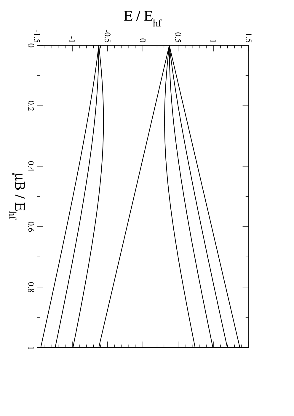
As an illustration, we take ⁸⁷Rb atoms, whose nuclear spin quantum number is $i={3\over 2}$. Since Rb is the $5^{\rm th}$ alkali atom, the energy scale of its first electronic excitation is approximately $E_{\rm Rydberg}/5^{2}\approx 0.55$ eV. At $B=0$, the electronic ground state is split into hyperfine multiplets with $f=1$ and $f=2$, with the $f=2$ multiplet higher in energy by $E_{\rm hf}=2.83\times 10^{-5}$ eV. Thus the hyperfine splitting is more than 4 orders of magnitude smaller than the energy scale for electronic excitations. The magnetic moment $\mu$ of a Rb atom is approximately that of an electron: $\mu\approx 2\mu_{B}$, where $\mu_{B}$ is the Bohr magneton. The magnetic energy scale $\mu B$ is comparable to $E_{\rm hf}$ when $B$ is about 2400 Gauss. The dependence of the hyperfine energy levels on the magnetic field is illustrated in Fig. 1.

If the atoms have sufficiently low energy that none of their electronic excitations can be excited, they can be described as point particles with multiple spin states that interact nonlocally through a potential. In the case of two alkali atoms, their interactions at sufficiently low energies can be described by the Born-Oppenheimer potentials $V_{s}(r)$ and $V_{t}(r)$ for atoms whose valence electrons are in spin-singlet and spin-triplet states, respectively. The spin-dependent potential can be written as an outer-product operator acting on the space of 2-atom spin states $|m_{s},m_{i}\rangle\otimes|m_{s}^{\prime},m_{i}^{\prime}\rangle$:

The asymptotic behaviors of the two potentials at large $r$ are

where $E_{0}$ is the scattering threshold for two atoms in the absence of the hyperfine and magnetic interactions. The scattering thresholds are split by the hyperfine and magnetic interactions in Eqs. (1) and (3). The threshold for two atoms in the states $|f,m_{f};B\rangle$ and $|f^{\prime},m_{f}^{\prime};B\rangle$ is $2E_{0}+E_{f,m_{f}}(B)+E_{f^{\prime},m_{f}^{\prime}}(B)$.

There are also 3-body and higher $n$-body interactions between atoms. Their effects are generally believed to be negligible in most cases, and we will ignore them. We will also ignore relativistic effects and retardation effects, which change the ultimate asymptotic behavior of the van der Waals potential from $1/r^{6}$ to $1/r^{7}$.

The nucleus of an atom with atomic number $Z$ and atomic mass number $A$ contains $Z$ protons and $A-Z$ neutrons. The atom also contains $Z$ electrons to neutralize the electric charge. Thus the total number of fermionic constituents in the atom is $A+Z$. The atom is a boson if $A+Z$ is even and a fermion if $A+Z$ is odd. In the case of alkali atoms, the atomic number $Z$ is always odd. Thus an alkali atom is a boson if $A$ is odd and a fermion if $A$ is even.

If two atoms are in the same spin state $|f,m_{f};B\rangle$, their wavefunction $\psi(\bm{r}_{1},\bm{r}_{2})$ must satisfy a symmetrization condition. If the atom is a boson, the wavefunction must be symmetric under interchange of the two coordinates: $\psi(\bm{r}_{2},\bm{r}_{1})=+\psi(\bm{r}_{1},\bm{r}_{2})$. If the atom is a fermion, the wavefunction must be antisymmetric under interchange of the two coordinates. More generally, two atoms can be in superpositions of the various hyperfine states, in which case their wavefunction has multiple components $\psi_{m_{s1}m_{i1},m_{s2}m_{i2}}(\bm{r}_{1},\bm{r}_{2})$. The symmetrization condition must be applied to the spin quantum numbers as well as to the coordinate dependence of the wavefunction. If the atom is a boson, the components of the wavefunction must satisfy

We can now specify the fundamental theory. The Hamiltonian is the sum of a one-body term for every particle and a 2-body term for every pair of particles. The one-body term is the sum of the kinetic energy $\bm{P}^{2}/(2m)$, the hyperfine term in Eq. (1), and the magnetic term in Eq. (3). The 2-body potentials are given in Eq. (6). The bosonic or fermionic nature of the atoms is implemented through constraints on the states. If the atom is a boson, the $N$-particle wavefunction must be symmetric under interchange of any pair of atoms. If the atom is a fermion, the $N$-particle wavefunction must be antisymmetric under such an interchange.

The fundamental theory can be formulated as a quantum field theory. This formulation involves $2(2i+1)$ quantum fields $\psi_{m_{s}m_{i}}(\bm{r})$ that can be arranged into a column vector $\Psi(\bm{r})$. The Hamiltonian is

where $r_{12}=|\bm{r}_{1}-\bm{r}_{2}|$. We have set $\hbar=1$ to simplify the expression. Dimensional analysis can be used to reintroduce $\hbar$ if desired. The quantum fields $\psi_{m_{s}m_{i}}(\bm{r})$ satisfy equal-time commutation relations. If the atom is a boson, the commutation relations are

If the atom is a fermion, the commutation relations are replaced by anti-commutation relations. The commutation relations imply that the quantum field $\psi_{m_{s}m_{i}}(\bm{r})$ annihilates an atom in the spin state $|m_{i},m_{s}\rangle$ at the point $\bf r$. They also enforce the constraint that quantum states must be symmetric under interchange of two atoms in the same spin state.

The fundamental theory has several symmetries:

• •

  phase symmetry. The Hamiltonian $H_{\rm fun}$ is invariant under phase transformations: $\Psi(\bm{r})\to e^{i\theta}\Psi(\bm{r})$. This symmetry is associated with the conservation of the number of atoms.

• •

  translational symmetry. If the magnetic field $\bm{B}(t)$ is homogeneous, $H_{\rm fun}$ is invariant under translations in space: $\bm{r}\to\bm{r}+\bm{a}$. This implies the conservation of the total momentum $\bm{P}$.

• •

  time translational symmetry. If the magnetic field $\bm{B}(\bm{r})$ is static, the theory is invariant under translations in time: $t\to t+a$. This implies the conservation of the total energy $E$, which is the eigenvalue of the Hamiltonian $H_{\rm fun}$.

• •

  rotational symmetry. The Hamiltonian is invariant under rotations generated by the total angular momentum operator $\bm{J}=\bm{L}+\bm{S}+\bm{I}$, where $\bm{L}$ is the orbital angular momentum, provided the magnetic field $\bm{B}$ is also transformed by the rotation. If $\bm{B}=0$, this symmetry implies the conservation of the total angular momentum $\bm{J}$. If $\bm{B}=B\bm{\hat{z}}$, it implies the conservation of the component $J_{z}$.

• •

  parity symmetry. The Hamiltonian is invariant under the reflection $\bm{r}\to-\bm{r}$.

The fundamental theory also has Galilean symmetry. Since the Hamiltonian is the generator of translations in time, the column vector of quantum fields can be extended to a time-dependent operator $\Psi(\bm{r},t)$:

The transformation of this time-dependent operator under a Galilean boost with velocity vector $\bm{v}$ is

This symmetry is not associated with a conservation law, because its generators do not commute with the Hamiltonian.

If we restrict our attention to low energies with respect to a given scattering threshold, the fundamental theory has additional approximate symmetries. If the atoms have sufficiently low kinetic energy, their total orbital angular momentum $\bm{L}$ can be neglected. If $\bm{B}=0$, the total hyperfine spin $\bm{F}=\bm{I}+\bm{S}$ is then conserved. If there is a nonzero magnetic field $\bm{B}=B\bm{\hat{z}}$, the component $F_{z}$ is conserved. The restriction on the energy may also impose a restriction on the possible spin states of the atoms. In this case, the conservation of total atom number may be replaced by a more restrictive conservation law. If $B=0$, the energy restriction could allow only atoms in a specific hyperfine multiplet with quantum number $f$, in which case the total number of atoms in those $2f+1$ hyperfine states will be conserved. If $B$ is large, the energy restriction may require all the atoms to be in the same spin state, in which case the number of atoms in that spin state will be conserved.

If two atoms in the hyperfine states $|f_{1},m_{f1};B\rangle$ and $|f_{2},m_{f2};B\rangle$ collide, they can either scatter elastically or they can scatter into a different pair of hyperfine states $|f_{1}^{\prime},m_{f1}^{\prime};B\rangle$ and $|f_{2}^{\prime},m_{f2}^{\prime};B\rangle$. The scattering rate for each scattering channel is determined by the $T$-matrix element, which is a function of the relative wavenumbers $\bm{k}$ and $\bm{k}^{\prime}$ for the initial and final states. If the collision energy relative to the scattering threshold is sufficiently small, elastic scattering is dominated by the $S$-wave orbital angular momentum channel and the $T$-matrix element ${\mathcal{T}}_{f_{1}m_{f1},f_{2}m_{f2}}(k)$ for elastic scattering reduces to a function of $k=|\bm{k}|=|\bm{k}^{\prime}|$ only. The low-energy limit of the $T$-matrix element is given by the scattering lengths for the hyperfine channel. If the two hyperfine states are distinct, we denote the scattering length by $a_{f_{1}m_{f1},f_{2}m_{f2}}$. The low-energy limit of the $T$-matrix element is

If the two atoms are in the same hyperfine state $|f,m_{f};B\rangle$, we denote the scattering length by $a_{fm_{f}}$. The low-energy limit of the $T$-matrix element is

If the atoms are fermions, the scattering length $a_{fm_{f}}$ vanishes because the wavefunction for an S-wave state must be symmetric under interchange of the coordinates. The cross section for the scattering of distinct hyperfine states are obtained by squaring the T-matrix element ${\mathcal{T}}_{f_{1}m_{f1},f_{2}m_{f2}}(k)$ and multiplying it by the flux factor $m/(2k)$ and by the phase space factor $mk/(2\pi)$. If the two atoms are in the same hyperfine state, the phase space factor is multiplied by a factor of ${1\over 2}$ to compensate for the double-counting of the states of the identical particles. Thus the low-energy limit of the cross section for the elastic scattering of two atoms in the $|f,m_{f};B\rangle$ hyperfine state is

In the absence of the hyperfine and magnetic interactions, scattering through the spin-singlet and spin-triplet potentials in Eq. (6) determines the spin-singlet and spin-triplet scattering lengths $a_{s}$ and $a_{t}$. The spin-triplet scattering length $a_{t}$ is the scattering length for a pair of atoms that are both in the same hyperfine state given in Eq. (4). The only effect of the hyperfine and magnetic terms on this channel is to change the scattering threshold. If it were not for the hyperfine term in Eq. (1), the scattering lengths for all the other hyperfine channels could be expressed as linear combinations of $a_{s}$ and $a_{t}$ using Clebsch-Gordon coefficients. Because of the hyperfine term, it is necessary to solve the coupled-channel Schrödinger equation numerically to determine the scattering lengths for all the other hyperfine channels. However, if the scattering lengths $a_{s}$ and $a_{t}$ are known, there is a simple approximation to the coupled-channel problem that reproduces the low-energy scattering observables, including the scattering lengths, quite accurately [1]. As illustrated in Fig. 2, the spin-singlet and spin-triplet potentials $V_{s}(r)$ and $V_{t}(r)$ in Eq. (6) can be replaced by their asymptotic forms in Eq. (7) together with boundary conditions at a small separation $r_{0}$. The boundary conditions are tuned so that the spin-singlet and spin-triplet scattering lengths have the desired values $a_{s}$ and $a_{t}$ for $B=0$ and $E_{\rm hf}=0$. Those same boundary conditions are then used for nonzero values of $B$ and $E_{\rm hf}$. Thus the low-energy scattering problem for all the hyperfine channels is essentially determined by just 5 parameters: $a_{s}$, $a_{t}$, $C_{6}$, $E_{\rm hf}$, and $\mu B$.

We now focus on a specific hyperfine channel. To be definite, we take the alkali atom to be a boson. We also take the two atoms to be in the same hyperfine state $|f,m_{f};B\rangle$, so they are identical bosons. We choose the origin of energy to be the scattering threshold for that channel: $2E_{0}+2E_{f,m_{f}}(B)$. The T-matrix element for S-wave scattering of two particles with collision energy $E=k^{2}/m$ can be expressed in the form

where $\delta_{0}(k)$ is the S-wave phase shift. If there are no lower hyperfine channels into which the atoms can scatter, the unitarity of the S-matrix implies that the phase shift is real valued. The low-energy behavior of the phase shift is given by the effective range expansion:

which defines the scattering length $a=a_{fm_{f}}$ and the effective range $r_{s}$. Taking the limit $k\to 0$ in Eq. (16) and using Eq. (17), we recover the limiting expression for the T-matrix element in Eq. (14).

If the fundamental theory had only short-range potentials, $k\cot\delta_{0}(k)$ would be an analytic function of $k^{2}$ at $k=0$ and it would therefore have a power series expansion in $k^{2}$. However, the asymptotic behavior of the potentials $V_{s}(r)$ and $V_{t}(r)$, as given in Eq. (7), is $1/r^{6}$. As a consequence, beginning at order $k^{4}$, there are logarithms of $k$ in the coefficients of the powers of $k$. Thus $k\cot\delta_{0}(k)$ has a well-behaved expansion in powers of $k^{2}$ only to order $k^{2}$. Thus the scattering length and the effective range defined by Eq. (17) are the only well-defined coefficients in the effective range expansion for atoms.

The important energy scales for low-energy alkali atoms include the hyperfine splitting $E_{\rm hyperfine}$, the magnetic energy scale $\mu B$, and the van der Waals energy scale defined by

For Rb atoms, the van der Waals energy scale is $E_{\rm vdW}=6.4\times 10^{-9}$ eV. This is more than 3 orders of magnitude smaller than the hyperfine splitting $E_{\rm hf}$. The magnetic energy scale $\mu B$ is comparable to $E_{\rm vdW}$ when the magnetic field is about 0.54 Gauss. The van der Waals energy scale corresponds to a temperature of $7.4\times 10^{-5}$ K. We consider atoms to be ultracold if their kinetic energies are much smaller than the van der Waals energy scale. In subsequent sections, we will review scattering models that can describe such ultracold atoms.

The natural scale for the scattering length $a$ of a specific hyperfine state is the van der Waals length defined by

A scattering length can be orders of magnitude larger than $\ell_{\rm vdw}$ only if there is a fine-tuning of some parameter in the Hamiltonian. If $|a|$ is much larger than $\ell_{\rm vdw}$, we refer to $a$ as a large scattering length. If $a$ is large, ultracold atoms have an important energy scale that is much smaller than the van der Waals energy scale $E_{\rm vdw}$, namely $\hbar^{2}/(ma^{2})$.

For particles with short-range interactions, the scattering length $a$ is considered to be large if its absolute value is much larger than the range. Particles with large scattering lengths have universal low-energy properties that depend on the scattering length but are insensitive to other details of the interactions. The known universal properties have been summarized in a recent review [2]. In the case of atoms, the relevant range is the van der Waals length scale $\ell_{\rm vdw}$ defined in Eq. (19). In the 2-atom sector, the universal properties are rather simple. The cross section for elastic scattering of bosonic atoms in the same spin state with energy in the region $|E|\ll E_{\rm vdW}$, where $E_{\rm vdW}$ is the van der Waals energy scale defined in Eq. (18), is given by the universal formula

Shallow bound states whose binding energies are much smaller than $E_{\rm vdW}$ are also universal. If $a<0$, there are no such bound states. If $a>0$, there is a single shallow bound state with binding energy

We will refer to this state as the shallow dimer.

The natural scale for the scattering lengths $a_{s}$ and $a_{t}$ is the van der Waals length defined in Eq. (19). The scattering length $a_{s}$ or $a_{t}$ can be much larger than $\ell_{\rm vdw}$ only if the depth of the potential $V_{s}(r)$ or $V_{t}(r)$ is tuned so that there is a bound state very close to the threshold. If $a_{s}$ or $a_{t}$ is large, several of the scattering lengths $a_{fm_{f}}$ of the hyperfine channels will also be large. Examples of alkali atoms that have large scattering lengths at zero magnetic field are ⁶Li ($a_{t}\approx-2160~a_{0}$), ⁸⁵Rb ($a_{s}\approx+2800~a_{0}$), and ¹³³Cs ($a_{t}\approx+2400~a_{0}$).

A large scattering length $a_{fm_{f}}$ in a specific hyperfine channel can be obtained by tuning the magnetic field $B$ to a Feshbach resonance $B_{i}$. If the magnetic field is near $B_{i}$, there is a diatomic molecule near the scattering threshold for two atoms in the $|f,m_{f};B\rangle$ hyperfine state. The diatomic molecule is a bound state of atoms in a spin state with a higher threshold. Since the magnetic moment of the diatomic molecule differs from twice the magnetic moment of the $|f,m_{f};B\rangle$ atom, the energy of the molecule can be made to cross the scattering threshold by changing the magnetic field $B$. The Feshbach resonance occurs at the value $B_{i}$ for which the molecule is at resonance with two atoms at the scattering threshold. The existence of Feshbach resonances in Cs atoms was first pointed out by Tiesinga, Verhaar, and Stoof [3]. The first Feshbach resonances to be observed were the resonances at 853 G and 907 G for ²³Na atoms in the $|1,-1\rangle$ hyperfine level [4] and the resonance at 155 G for ⁸⁵Rb atoms in the $|2,-2\rangle$ hyperfine level [5]. The physics of Feshbach resonances in cold atoms has been summarized in a recent review [6].

At a generic value $B_{0}$ of the magnetic field, the scattering length $a(B)$ for a specific hyperfine channel varies slowly as a function of the magnetic field $B$. It can therefore be expanded as a power series around $B=B_{0}$:

At a Feshbach resonance, the scattering length is not a smooth function of $B$. When the magnetic field is well below the Feshbach resonance $B_{i}$, the scattering length has some off-resonant value $a_{\rm bg}$. As $B$ increases through the value $B_{i}$, $a(B)$ diverges to $+\infty$ or $-\infty$, jumps discontinuously to $-\infty$ or $+\infty$, and then approaches the original off-resonant value $a_{\rm bg}$. The scattering length must pass through zero at some value of $B$, either before or after $B_{i}$. If we denote that value by $B_{i}+\Delta_{i}$, the scattering length can be expressed as

where $a_{\rm bg}(B)$ is a smooth function of the magnetic field that can be expanded as a power series around $B_{i}$ as in Eq. (22). The parameters $B_{i}$ and $\Delta_{i}$ are convenient, because it is often possible to measure the locations of divergences and zeroes of the scattering length more accurately than its value $a(B)$ at any particular value of $B$.

One class of models that can be used to describe the behavior of ultracold atoms in the spin state of interest is potential models. A potential model is specified by interaction potentials between the constituents of the model. In the simplest potential models, the only constituents are atoms in the spin state of interest. In this case, the potential model is specified by a single potential $V(r)$. The potential $V(r)$ must be tuned so that the solutions to the single-channel Schrödinger equation for that potential give the same results for low-energy scattering cross sections and low-energy bound states as the solution to the coupled-channel Schrödinger equation for the fundamental theory. The potential $V(r)$ need not resemble either of the potentials $V_{s}(r)$ or $V_{t}(r)$ in the fundamental theory as long as it accurately reproduces low-energy observables for atoms in the spin state of interest. If we restrict our attention to sufficiently low energies that the scattering length $a$ is the only relevant interaction parameter, then all that is required is that the potential be short-ranged and give the correct scattering length.

A potential model can be formulated as a quantum field theory. If the only constituents in the model are atoms in a single hyperfine state $|f,m_{f};B\rangle$, there is a single quantum field $\psi(\bm{r})$ which annihilates atoms in that hyperfine state. The Hamiltonian is

The time-dependent quantum field $\psi(\bm{r},t)$ satisfies equal-time commutation relations. If the atom is a boson, the commutation relations are

A more elaborate potential model could describe $N-1$ additional spin states of the atoms. The model would be specified by the diagonal potentials for each pair of spin states and by coupling potentials between pairs of spin states. These potentials need not resemble those of the fundamental theory as long as the solutions to the Schrödinger equation for all the coupled channels reproduce the predictions of the fundamental theory for low-energy observables involving the spin state of interest.

Another class of models that can be used to describe the low-energy behavior of the atoms is scattering models. A scattering model can be specified by the $T$-matrix elements for scattering of the constituents of the model along with any additional parameters that are required to make the model well-defined. In the simplest scattering models, the only constituents are atoms in a single spin state. At sufficiently low energies, the atoms have only S-wave scattering and the T-matrix element reduces to a function ${\mathcal{T}}(k)$ of the magnitude of the relative momentum $k$ only. Since it is specified in terms of the low-energy observables ${\mathcal{T}}(k)$, a scattering model provides a particularly natural description for ultracold atoms.

A more elaborate scattering model could include other spin states of the atom as additional degrees of freedom. In this case, the T-matrix elements for all the pairs of spin states could be part of the specification of the model. In contrast to potential models, diatomic molecules can also be included as explicit degrees of freedom in a scattering model. In this case, T-matrix elements involving the diatomic molecules could also be part of the specification of the model.

A scattering model can be formulated as a quantum field theory. If the T-matrix element ${\mathcal{T}}(k)$ that is part of the specification of the scattering model is an analytic function of $k^{2}$ at $k=0$, the T-matrix element can be reproduced by a local quantum field theory. A local quantum field theory is one whose interactions only involve the quantum fields and their derivatives at the same point in space. If a local quantum field theory has a Hamiltonian formulation, its Hamiltonian can be expressed as the integral over space of a Hamiltonian density:

If the quantum field $\psi(\bm{r})$ that annihilates atoms in the spin state of interest is the only quantum field in the model, the free term in the Hamiltonian density is

The interaction term in the Hamiltonian density must be a polynomial in $\psi$ and $\psi^{\dagger}$ and their gradients, such as

One advantage of a Hamiltonian quantum field theory is that it guarantees that the space of quantum states is a Hilbert space. Since the Hamiltonian $H$ is a hermitian operator, its eigenstates $|n\rangle$ form a complete set of states. The completeness relation can be expressed formally as $\sum_{n}|n\rangle\langle n|=1$. If we express the S-matrix in the form ${\mathcal{S}}=1+i{\mathcal{T}}$, the completeness relation can be used to express the unitarity condition ${\mathcal{S}}^{\dagger}{\mathcal{S}}=1$ in the form

This form of the unitarity condition is called the Optical Theorem. Note that the right side is the sum of positive-definite terms.

It is sometimes useful to consider a more general class of quantum field theories that have a Lagrangian formulation but do not necessarily have a Hamiltonian formulation. The Lagrangian for a local quantum field theory can be expressed as the integral over space of a Lagrangian density:

If the quantum field $\psi(\bm{r})$ that annihilates atoms in the spin state of interest is the only quantum field in the model, the free term in the Lagrangian density is

This form is manifestly real. If we ignore terms that are total time derivatives or total divergences, it can be written in a more compact form:

If the quantum field theory has a Hamiltonian formulation, the interaction term in the Lagrangian density is simply ${\mathcal{L}}_{\rm int}=-{\mathcal{H}}_{\rm int}$. However, Lagrangian quantum field theories are a more general class of models than Hamiltonian quantum field theories. They can, for example, have interaction terms that involve time derivatives, such as

More generally, ${\mathcal{L}}_{\rm int}$ must be a polynomial in $\psi$, $\psi^{\dagger}$, their gradients, and their time-derivatives.

If all we have is a Lagrangian formulation of the quantum field theory, there is no guarantee that the Optical Theorem will have the form in Eq. (29), where ${\rm Im}\,\langle i|{\mathcal{T}}|i\rangle$ is expressed as the sum of positive-definite terms. The general expression may have the form

where the states labeled $|n\rangle$ and $|m\rangle$ together form a complete set. One way to interpret such a relation is that the space of quantum states is a complex vector space with indefinite norm. The completeness relation for this vector space has the form $\sum_{n}|n\rangle\langle n|-\sum_{m}|m\rangle\langle m|=1$. The states $|m\rangle$ can be interpreted as states with negative norm.

The problem of negative-norm states arises in covariant formulations of Quantum Electrodynamics. However, one can use gauge invariance to show that there is a physical subspace of the complex vector space spanned by the positive-norm states $|n\rangle$ such that if $|i\rangle$ is in the physical subspace, ${\rm Im}\,\langle i|{\mathcal{T}}|i\rangle$ can be written as the sum of positive-definite terms:

This requires a cancelation between positive and negative terms in Eq. (34). In QED, this cancelation is guaranteed by gauge invariance. In a scattering model for atoms, there is no obvious mechanism to guarantee such a cancelation. Thus the existence of negative-definite terms in the imaginary part of a diagonal T-matrix element is more problematic.

The symmetries of the fundamental theory can be used to constrain the Hamiltonian or the Lagrangian of a local quantum field theory. We will give the constraints only for the simple case of a single quantum field $\psi(\bm{r},t)$:

• •

  phase symmetry. The phase transformation is $\psi(\bm{r},t)\to e^{i\theta}\psi(\bm{r},t)$. Invariance under this transformation requires that every term in ${\mathcal{H}}_{\rm int}$ or ${\mathcal{L}}_{\rm int}$ have an equal number of factors of $\psi$ and $\psi^{\dagger}$.

• •

  translational symmetry. This is implemented automatically in a local quantum field theory for which ${\mathcal{H}}_{\rm int}$ or ${\mathcal{L}}_{\rm int}$ is a function of $\psi$, $\psi^{\dagger}$, their gradients, and their time-derivatives.

• •

  time translational symmetry. This is also implemented automatically in a local quantum field theory.

• •

  rotational symmetry. If the model involves only a single quantum field $\psi(\bm{r},t)$, a rotation acts only on its vector argument $\bm{r}$. The requirement of rotational symmetry is that ${\mathcal{H}}_{\rm int}$ or ${\mathcal{L}}_{\rm int}$ be a scalar under rotations. This requires each gradient $\nabla^{i}$ to have its index $i$ contracted with that of another gradient $\nabla^{i}$ or with a Levi-Civita tensor $\epsilon^{ijk}$.

• •

  parity symmetry. This can be used to exclude terms in ${\mathcal{H}}_{\rm int}$ or ${\mathcal{L}}_{\rm int}$ with a Levi-Civita tensor.

Galilean symmetry imposes strong constraints on the interaction terms in ${\mathcal{H}}_{\rm int}$ or ${\mathcal{L}}_{\rm int}$. The Galilean transformation with velocity vector $\bm{v}$ in the fundamental theory is given in Eq. (12). The corresponding Galilean transformation for the field $\psi(\bm{r},t)$ is

One way to construct interaction terms that are Galilean invariant is to construct them out of building blocks with simple behavior under Galilean transformations. One simple building block is the product $\psi^{\dagger}\psi$, which is Galilean invariant. Thus terms constructed out of $\psi^{\dagger}\psi$ and its gradients, such as $\nabla^{i}(\psi^{\dagger}\psi)$ and $\nabla^{i}\nabla^{j}(\psi^{\dagger}\psi)$, are Galilean invariant. The first term in ${\mathcal{H}}_{\rm int}$ in Eq. (28) is Galilean invariant, because it can be expressed as $(\psi^{\dagger}\psi)^{2}$. The second term in ${\mathcal{H}}_{\rm int}$ is also Galilean invariant, because it can be expressed in the form $\nabla(\psi^{\dagger}\psi)\cdot\nabla(\psi^{\dagger}\psi)$.

Another simple building block is $\psi{\stackrel{{\scriptstyle\leftrightarrow}}{{\nabla}}}{}^{2}\psi$, where the operator $\stackrel{{\scriptstyle\leftrightarrow}}{{\nabla}}{}^{2}$ is defined by

The operator $\psi{\stackrel{{\scriptstyle\leftrightarrow}}{{\nabla}}}{}^{2}\psi$ transforms under Galilean transformations in the same way as $\psi^{2}$. A further set of simple building blocks is the combination $[i\frac{\partial}{\partial t}+\nabla^{2}/(2Nm)]\psi^{N}$, where $N=1,2,\ldots$. They transform under Galilean transformations in the same way as $\psi^{N}$. This combination with $N=1$ appears in the expression for ${\mathcal{L}}_{\rm free}$ in Eq. (32). This combination with $N=2$ appears in the interaction term in Eq. (33).

If the energy restriction allows atoms in multiple spin states related by a symmetry, the symmetry can be imposed on the corresponding quantum fields $\psi_{m}(\bm{r},t)$. For example, if $B=0$, the $2f+1$ spin states in a hyperfine multiplet form an irreducible $(2f+1)$-dimensional representation of the $SU(2)$ symmetry group of angular momentum. There is also a $U(1)$ symmetry corresponding to multiplying all the fields $\psi_{m}(\bm{r},t)$ by the same phase.

In a quantum field theory, physical observables can be conveniently encoded in the correlation functions of the theory. The physical observables in the 2-atom sector can be encoded in the amputated connected Green’s function ${\mathcal{A}}$ for two atoms in the asymptotic past to evolve into two atoms in the asymptotic future. In general, this amplitude is a function of the energies $E_{1}$ and $E_{2}$ and the momenta $\bm{p}_{1}$ and $\bm{p}_{2}$ of the two incoming atoms and the energies $E_{1}^{\prime}$ and $E_{2}^{\prime}$ and the momenta $\bm{p}_{1}^{\prime}$ and $\bm{p}_{2}^{\prime}$ of the two outgoing atoms. The atoms can be off their energy shells: $E_{i}$ need not be equal to $p_{i}^{2}/(2m)$. The total energy $E$ and the total momentum $\bm{P}$ are conserved: $E_{1}+E_{2}=E_{1}^{\prime}+E_{2}^{\prime}=E$ and $\bm{p}_{1}+\bm{p}_{2}=\bm{p}_{1}^{\prime}+\bm{p}_{2}^{\prime}=\bm{P}$. Galilean invariance constrains the amplitude to be a function of $E-\bm{P}^{2}/(4m)$ and the relative momenta $\bm{k}={1\over 2}(\bm{p}_{1}-\bm{p}_{2})$ and $\bm{k}^{\prime}={1\over 2}(\bm{p}_{1}^{\prime}-\bm{p}_{2}^{\prime})$. We can simplify the problem by working in the center-of-mass frame $\bm{P}=0$. If the energy is restricted to be low enough that there is S-wave scattering only, the amplitude in the center-of-mass frame depends only on the magnitudes of $\bm{k}$ and $\bm{k}^{\prime}$, so it reduces to a function ${\mathcal{A}}(E;k,k^{\prime})$ of three variables.

The amplitude ${\mathcal{A}}(E;k,k^{\prime})$ encodes all information about low-energy 2-atom scattering. The T-matrix element ${\mathcal{T}}(k)$ for the S-wave scattering of two atoms with relative momentum $\bm{k}$ into two atoms with relative momentum $\bm{k}^{\prime}$ is obtained by evaluating ${\mathcal{A}}(E;k,k^{\prime})$ at the on-shell point obtained by setting all the atoms on their energy shells: $E=2(k^{2}/2m)=2({k^{\prime}}^{2}/2m)$, which requires $k=k^{\prime}$. The T-matrix element is

The cross section for the elastic scattering of two identical bosonic atoms with total kinetic energy $E=k^{2}/m$ is obtained by squaring the T-matrix element and multiplying by the phase space factor $mk/(4\pi)$ and by the flux factor $m/(2k)$:

Information about S-wave bound states is also encoded in ${\mathcal{A}}(E;k,k^{\prime})$ through its poles in the energy $E$. The amplitude ${\mathcal{A}}(E;k,k^{\prime})$ is a double-valued function of the energy variable $E$, which takes its values on the two-sheeted complex plane with a branch point at $E=0$ and a branch cut along the positive $E$ axis. The interpretation of the pole in $E$ depends on where the pole resides in the complex $E$ plane. For simplicity, we assume that the atom has no spin states with lower energy. A pole on the negative real axis of the physical sheet of the complex energy $E$ corresponds to a stable bound state. A pole on the negative real axis of the unphysical sheet is called a virtual state. A pole on the unphysical sheet just below the positive real axis corresponds to a scattering resonance.

One complication of local quantum field theories is that they are inherently singular at short distances. The theory is well-defined only if it is modified in some way to suppress the effects of particles that approach arbitrarily close to each other or that have arbitrarily high energy. A convenient way to do this is to impose an upper limit on the wavevector of virtual particles: $|\bm{k}|<\Lambda$. The variable $\Lambda$ is called the ultraviolet cutoff. The singularities then appear in the limit $\Lambda\to\infty$. However, it is possible to avoid the singularities by using a procedure called renormalization. The parameters of the model, such as $\lambda_{0}$ and $\rho_{0}$ in Eq. (28), are made functions of $\Lambda$ in such a way that the model has a well-behaved and nontrivial limit as $\Lambda\to\infty$.

There are two rather different approaches to renormalization. The simplest approach conceptually is called Gell-Mann-Low renormalization. This is the approach that was followed in the original development of renormalized perturbation theory for Quantum Electrodynamics. A quantum field theory model can be specified by a Hamiltonian density with a finite number of interaction terms:

If the coupling constants $c_{n}(\Lambda)$ can be tuned as functions of the ultraviolet cutoff so that physical observables have well-behaved and nontrivial limits as $\Lambda\to\infty$, the model is called renormalizable. It may be necessary to add operators to the set $\{{\mathcal{O}}_{1},\ldots,{\mathcal{O}}_{N}\}$ or remove some of the operators to make the model renormalizable. In nonrelativistic quantum field theories in which the total number of particles cannot change, the physical observables can be classified according to the particle number. If the coupling constants can be tuned so that all $N$-particle observables have well-behaved limits as $\Lambda\to\infty$, the model is called renormalizable in the $N$-atom sector. If the model is renormalizable in the $N$-atom sector, it is renormalizable in the $n$-atom sector for all $n<N$. In this paper, we will for the most part consider only the constraints from renormalizability in the 2-atom sector.

The other approach to renormalization is called Wilsonian renormalization. This approach was followed by Ken Wilson when he developed the renormalization group to understand strongly-interacting quantum field theories. One begins by considering the most general model consistent with the symmetries. The Hamiltonian density in Eq. (40) is generalized to one with infinitely many operators ${\mathcal{O}}_{n}$, each with its own coupling constant $c_{n}(\Lambda)$. The free term ${\mathcal{H}}_{\rm free}$ is included as just another operator with a coupling constant $c_{\rm free}(\Lambda)$. We define the engineering dimension $d_{n}$ of an operator ${\mathcal{O}}_{n}$ by specifying the dimensions of $\psi$ and $\nabla$ to be $\frac{3}{2}$ and 1, respectively. For this purpose, the mass $m$ is treated as a dimensionless conversion factor. The engineering dimension of the free term in Eq. (27) is then 5. An $N$-atom operator with $N$ factors of $\psi$, $N$ factors of $\psi^{\dagger}$, and $D$ factors of the gradient $\nabla$ has engineering dimension $3N+D$. It is convenient to introduce dimensionless coupling constants $\hat{c}_{n}(\Lambda)$ defined by

The condition that low-energy observables defined by the Hamiltonian be independent of $\Lambda$ defines a flow on the infinite-dimensional space of dimensionless coupling constants $\hat{c}_{n}$. This flow can have a fixed point whose coordinates $c_{n}^{*}$ are independent of $\Lambda$. The corresponding fixed-point Hamiltonian ${\mathcal{H}}^{*}$ describes a scale-invariant system. Near the fixed point, a convenient basis of operators consists of scaling operators ${\mathcal{O}}_{n}^{*}$ that have the property that when their coupling constants are infinitesimally small, they scale as definite powers of $\Lambda$:

We refer to the exponent $\gamma_{n}$ as the scaling dimension of the operator ${\mathcal{O}}_{n}^{*}$. An operator with scaling dimension $\gamma_{n}<0$ is called relevant, because it becomes increasingly important as $\Lambda$ decreases towards 0 and thus has a dramatic effect on the physics at low energies. An operator with scaling dimension $\gamma_{n}>0$ is called irrelevant, because it decreases in importance as $\Lambda$ decreases towards 0. An operator with scaling dimension $\gamma_{n}=0$ is called marginal. The Hamiltonian density can be expanded around the fixed point in terms of the scaling operators:

Once the scaling operators have been identified and their scaling dimensions $\gamma_{n}$ determined, the model can be truncated to include only a finite number of terms in the Hamiltonian. A consistent truncation must include all the operators that are relevant and marginal. The behavior of the system near the fixed point can be described more accurately by including irrelevant operators. The accuracy of the description can be systematically improved by adding operators with increasing values of $\gamma_{n}$.

The simplest example of a renormalization group fixed point is the free theory with the Hamiltonian density ${\mathcal{H}}_{\rm free}$ in Eq. (27). This fixed point is called the trivial fixed point. The forms of the scaling operators depend on the choice of ultraviolet cutoff or regularization. With a scale-invariant regularization scheme, such as dimensional regularization, the scaling operators consist of terms that all have the same engineering dimensions. A scaling operator with $N$ factors of $\psi$, $N$ factors of $\psi^{\dagger}$, and $D$ factors of $\nabla$ has scaling dimension $3N+D-5$. The 2-body interaction terms in Eq. (28) are irrelevant operators with scaling dimensions 1 and 3, respectively. The simplest 3-body interaction term $(\psi^{\dagger})^{3}\psi^{3}$ is an irrelevant operator with scaling dimension 4. The successive truncation of the Hamiltonian to include operators with increasingly higher scaling dimension corresponds to a combination of the gradient expansion and an expansion in the number of particles.

The system of nonrelativistic particles with short-range interactions also has a nontrivial fixed point. In terms of the effective range expansion in Eq. (17), the fixed point corresponds to the limit in which the scattering length $a$ is infinite and the effective range $r_{s}$ and all higher coefficients in the expansion are 0. The dimensions of the scaling operators at the fixed point were deduced by Kaplan, Savage and Wise [7, 8] and by van Kolck [9]. There is a relevant operator with scaling dimension $-1$ which if added to the fixed-point Hamiltonian gives a model with a finite scattering length. There are also irrelevant operators with scaling dimensions 1, 3, 5, ….

The Zero-Range Model can be described by a quantum field theory with the single complex field $\psi$. The Hamiltonian density is the sum of the free term in Eq. (27) and the interaction term

The interaction term corresponds to a momentum-independent vertex with the Feynman rule $-i\lambda_{0}$. Such an interaction is singular, so the model requires an ultraviolet cutoff $\Lambda$ on the momenta of virtual atoms.

The Zero-Range Model is renormalizable in the 2-body sector. As shown in Sec. 4.2, the bare coupling constant $\lambda_{0}$ in Eq. (45) can be adjusted as a function of $\Lambda$ so that 2-body observables do not depend on $\Lambda$. The scattering length has the desired value $a$ if the bare coupling constant is

This expression can be inverted to express the scattering length as a function of the bare coupling constant and the cutoff:

The expression for the bare coupling constant in Eq. (46) provides a simple illustration of Wilsonian renormalization, which was discussed in Sec. 3.7. The operator $(\psi^{\dagger}\psi)^{2}$ in Eq. (45) has engineering dimension 6. The corresponding dimensionless coupling constant is therefore $\Lambda\lambda_{0}(\Lambda)$. This dimensionless coupling constant has fixed points for two values of the scattering length: $a=0$ and $a=\pm\infty$. The trivial fixed point $a=0$ corresponds to a noninteracting theory. For infinitesimal values of $a$, the dimensionless coupling constant is $\Lambda\lambda_{0}(\Lambda)\approx 8\pi a\Lambda/m$. Thus near the trivial fixed point, $(\psi^{\dagger}\psi)^{2}$ is an irrelevant operator with scaling dimension 1. The nontrivial fixed point $a=\pm\infty$ is commonly referred to as the unitary limit. At the fixed point, the dimensionless coupling constant is $\hat{\lambda}_{0}^{*}\approx-4\pi^{2}/m$. For infinitesimal values of $1/a$, the deviation of the dimensionless coupling constant from its fixed-point value is $\Lambda\lambda_{0}(\Lambda)-\hat{\lambda}_{0}^{*}\approx-2\pi^{3}/(ma\Lambda)$. Thus near the unitary fixed point, $(\psi^{\dagger}\psi)^{2}$ is a relevant operator with scaling dimension $-1$.

The amputated connected Green’s function for 2 atoms to evolve into 2 atoms can be calculated analytically by summing the series of diagrams shown in Fig. 3. Each vertex gives a factor of $-i\lambda_{0}$. Each loop gives the product of two propagators, which must be integrated over the momenta and energies of the virtual atoms. In the center-of-mass frame, the integral is

References

- [1] P.S. Julienne and B. Gao, “Simple Theoretical Models for Resonant Cold Atom Interactions,” arXiv:physics/06090, to be published in the Proceedings of the 20th International Conference on Atomic Physics, Innsbruck, Austria, July 2006.
- [2] E. Braaten and H. W. Hammer, “Universality in Few-body Systems with Large Scattering Length,” Phys. Rept. 428, 259 (2006) [arXiv:cond-mat/0410417].
- [3] E. Tiesinga, B.J. Verhaar, and H.T. Stoof, “Threshold and resonance phenomena in ultracold ground-state collisions,” Phys. Rev. A 47, 4114 (1993).
- [4] S. Inouye, M.R. Andrews, J. Stenger, H.-J. Miesner, D.M. Stamper-Kurn, and W. Ketterle, “Observation of Feshbach Resonances in a Bose-Einstein condensate,” Nature 392, 151 (1998).
- [5] Ph. Courteille, R.S. Freeland, D.J. Heinzen, F.A. van Abeelen, and B.J. Verhaar, “Observation of a Feshbach Resonance in Cold Atom Scattering,” Phys. Rev. Lett. 81, 69 (1998).
- [6] T. Köhler, K. Góral, and P.S. Julienne, “Production of cold molecules via magnetically tunable Feshbach resonances.” Rev. Mod. Phys. 78, 1311 (2006).
- [7] D.B. Kaplan, M.J. Savage and M.B. Wise, “A new expansion for nucleon nucleon interactions,” Phys. Lett. B 424, 390 (1998) [arXiv:nucl-th/9801034].
- [8] D.B. Kaplan, M.J. Savage and M.B. Wise, “Two-nucleon systems from effective field theory,” Nucl. Phys. B 534, 329 (1998) [arXiv:nucl-th/9802075].
- [9] U. van Kolck, “Effective field theory of short-range forces,” Nucl. Phys. A 645, 273 (1999) [arXiv:nucl-th/9808007].
- [10] V. Efimov, “Energy Levels Arising from Resonant Two-body Forces in a Three-body System,” Phys. Lett. 33B, 563 (1970).
- [11] V. Efimov, “Weakly-bound States of Three Resonantly-interacting Particles,” Sov. J. Nucl. Phys. 12, 589 (1971) [Yad. Fiz. 12, 1080 (1970)].
- [12] P. F. Bedaque, H. W. Hammer and U. van Kolck, “Renormalization of the three-body system with short-range interactions,” Phys. Rev. Lett. 82, 463 (1999) [arXiv:nucl-th/9809025].
- [13] P. F. Bedaque, H. W. Hammer and U. van Kolck, “The Three-Boson System with Short-Range Interactions,” Nucl. Phys. A 646, 444 (1999) [arXiv:nucl-th/9811046].
- [14] L. Platter, H. W. Hammer and U. G. Meissner, “The Four-Boson System with Short-Range Interactions,” Phys. Rev. A 70, 052101 (2004) [arXiv:cond-mat/0404313].
- [15] H. W. Hammer and L. Platter, “Universal Properties of the Four-Body System with Large Scattering Length,” Eur. Phys. J. A 32, 113 (2007) [arXiv:nucl-th/0610105].
- [16] D.R. Phillips, S.R. Beane and T.D. Cohen, “Nonperturbative regularization and renormalization: Simple examples from nonrelativistic quantum mechanics,” Annals Phys. 263, 255 (1998) [arXiv:hep-th/9706070].
- [17] C.J. Fewster, “Generalized point interactions for the radial Schrodinger equation via unitary dilations,” J. Phys. A 28, 1107 (1995) [arXiv:hep-th/9412050].
- [18] J.F. Yang and J.H. Huang, “Renormalization of scattering: contact potential,” Phys. Rev. C 71, 034001 (2005) [Erratum-ibid. C 71, 069901 (2005)] [arXiv:nucl-th/0409023].
- [19] D.B. Kaplan, M.J. Savage and M.B. Wise, “Nucleon-Nucleon Scattering from Effective Field Theory,” Nucl. Phys. B 478, 629 (1996) [arXiv:nucl-th/9605002].
- [20] M.C. Birse, J.A. McGovern and K.G. Richardson, “A renormalization-group treatment of two-body scattering,” Phys. Lett. B 464, 169 (1999) [arXiv:hep-ph/9807302].
- [21] K. Harada, K. Inoue and H. Kubo, “Wilsonian RG and Redundant Operators in Nonrelativistic Effective Field Theory,” Phys. Lett. B 636, 305 (2006) [arXiv:nucl-th/0511020].
- [22] K. Harada and H. Kubo, “Anomalous dimensions determine the power counting: Wilsonian RG analysis of nuclear EFT,” Nucl. Phys. B 758, 304 (2006) [arXiv:nucl-th/0605004].
- [23] K. Harada, H. Kubo and A. Ninomiya, “More about the Wilsonian analysis on the pionless NEFT,” arXiv:nucl-th/0702074.
- [24] T.D. Cohen, B.A. Gelman and U. van Kolck, “An effective field theory for coupled-channel scattering,” Phys. Lett. B 588, 57 (2004) [arXiv:nucl-th/0402054].
- [25] M. J. Savage, “The intermediate state in scattering from effective field theory,” Phys. Rev. C 55, 2185 (1997) [arXiv:nucl-th/9611022].
- [26] D.B. Kaplan, “More effective field theory for nonrelativistic scattering,” Nucl. Phys. B 494, 471 (1997) [arXiv:nucl-th/9610052].
- [27] S.J.J.M.F. Kokkelmans, J.N. Milstein, M.L. Chiofalo, R. Walser, and M.J. Holland, “Resonance superfluidity: Renormalization of resonance scattering theory,” Phys. Rev. A 65, 053617 (2002).