Hard spectator interactions in
at order
Volker Pilipp
Dissertation
an der Fakultät für Physik
der Ludwig–Maximilians–Universität
München
vorgelegt von
Volker Pilipp
aus München
München, den 31. Mai 2007
Erstgutachter: Prof. Dr. Gerhard Buchalla
Zweitgutachter: Priv. Doz. Dr. Stefan Dittmaier
Tag der mündlichen Prüfung: 30. Juli 2007
Zusammenfassung
In der vorliegenden Arbeit diskutiere ich die hard spectator interaction Amplitude von zur nächstführenden Ordnung in QCD (d.h. ). Dieser spezielle Teil der Amplitude, dessen führende Ordnung bei beginnt, ist im Rahmen der QCD Faktorisierung definiert. QCD Faktorisierung ermöglicht, in führender Ordnung in einer Entwicklung in die kurz- und die langreichweitige Physik zu trennen, wobei die kurzreichweitige Physik in einer störungstheoretischen Entwicklung in berechnet werden kann. Gegenüber anderen Teilen der Amplitude erfahren hard spectator interactions formal eine Verstärkung durch die zusätzlich zur -Skala hinzutretende hartkollineare Skala , die zu einem größeren numerischen Wert von führt.
Aus rechentechnischer Sicht liegen die hauptsächlichen Herausforderungen dieser Arbeit in der Tatsache begründet, dass die Feynmanintegrale, mit denen wir es zu tun haben, bis zu fünf äußere Beine haben und drei unabhängige Skalenverhältnisse enthalten. Diese Feynmanintegrale müssen in Potenzen in entwickelt werden. Ich werde integration by parts Identitäten vorstellen, mit denen die Anzahl der Masterintegrale reduziert werden kann. Ebenso werde ich diskutieren, wie man mit Differenzialgleichungsmethoden die Entwicklung der Masterintegrale in erhält. Im Anhang ist eine konkrete Implementierung der integration by parts Identitäten für ein Computeralgebrasystem vorhanden.
Schließlich diskutiere ich numerische Sachverhalte, wie die Abhängigkeit der Amplituden von der Renormierungsskala und die Größe der Verzweigungsverhältnisse. Es wird sich herausstellen das die nächstführende Ordnung der hard spectator interactions wichtig jedoch klein genug ist, so dass die Gültigkeit der Störungstheorie bestehen bleibt.
Abstract
In the present thesis I discuss the hard spectator interaction amplitude in at NLO i.e. at . This special part of the amplitude, whose LO starts at , is defined in the framework of QCD factorization. QCD factorization allows to separate the short- and the long-distance physics in leading power in an expansion in , where the short-distance physics can be calculated in a perturbative expansion in . Compared to other parts of the amplitude hard spectator interactions are formally enhanced by the hard collinear scale , which occurs next to the -scale and leads to an enhancement of .
From a technical point of view the main challenges of this calculation are due to the fact that we have to deal with Feynman integrals that come with up to five external legs and with three independent ratios of scales. These Feynman integrals have to be expanded in powers of . I will discuss integration by parts identities to reduce the number of master integrals and differential equations techniques to get their power expansions. A concrete implementation of integration by parts identities in a computer algebra system is given in the appendix.
Finally I discuss numerical issues like scale dependence of the amplitudes and branching ratios. It will turn out that the NLO contributions of the hard spectator interactions are important but small enough for perturbation theory to be valid.
Chapter 1 Introduction
The present situation of particle physics is the following. On the one hand we have got an extremely successful standard model that describes physics up to energy scales current accelerators are able to reach. On the other hand it has limitations and problems, e.g. the arbitrariness of the standard model parameters, the fact that the Higgs particle has not yet been found, the stabilisation of the Higgs mass under loop corrections (fine tuning problem) or the question why the electroweak scale is so much lower than the Planck scale (hierarchy problem). So most particle physicists expect new physics to show up at energy scales that are beyond the range of present accelerators but will be reached by future colliders. Within the next year LHC at CERN will start running and in the following years will collect data from proton proton collisions at a centre of mass energy of 14 TeV. This will allow us to obtain information about new physics by producing not yet observed particles directly. On the other hand physics beyond the standard model can be discovered by precision measurements of low energy quantities which are influenced by new physics particles because of quantum effects. The currently running experiments BaBar and Belle and after the start of LHC also LHCb are dedicated to examine decays of -mesons, where new physics is expected to be seen in CP asymmetries.
However in order to find new physics by indirect search, some parameters of the standard model have to be determined more precisely. To this end LHCb will make an important contribution. Above all the Wolfenstein parameters and [1, 2] that occur in the parametrisation of the Cabibbo-Kobayashi-Maskawa (CKM) matrix and determine its complex phase, which leads to CP asymmetry in the standard model, are up to now only very imprecisely known [3]:
| (1.1) |
These parameters, which influence weak interactions of quarks, can be determined with higher accuracy by -meson decays. In order to reduce their large uncertainties on the experimental side better statistics is needed, which is expected to be improved in the next few years, and on the theoretical side we have to get hadronic physics under control. This is due to the fact that weak interactions of quarks, from which and are measured, are always spoiled by non-perturbative strong interactions, because quarks are bound in hadronic states like mesons. Hadronic physics, however, is governed by the energy scale , where QCD cannot be handled perturbatively.
There are several advantages in observing -meson decays. One of them is due to the production of -mesons itself: There exists an extremely clean source to produce -mesons: The resonance , a bound state of a pair, has a mass that is only slightly larger than twice the mass of the -meson and decays nearly completely into pairs. This resonance is used at the -factories BaBar and Belle.
Another advantage is the possibility to obtain clean information about the complex phase of the CKM matrix by measurement of quantum mechanical oscillations in the system. The lifetime of -mesons, which is about , is large enough to observe those oscillations in the detector [4, 5]. By measuring the time dependent CP violation it is possible to obtain the CKM angles , and , which determine and , with small hadronic uncertainties (see e.g. chapter 1 of [6]). The “golden channel” , where the dependence on hadronic quantities is strongly suppressed by small CKM parameters, allows a quite precise determination of [7]. In the same way the decay could be used for a precise determination of the angle . However other than in the “golden channel” in the case of hadronic physics plays a subdominant but non-negligible role.
At this point another convenient property of the -meson comes into play. The mass of the -quark introduces a hard scale, at which is small enough to make perturbation theory possible. However the bound state of the -quark in the -meson is dominated by physics of the soft scale , where perturbation theory breaks down. While inclusive decays can be handled in the framework of operator product expansion, for exclusive decays, which the present thesis deals with, the framework of QCD factorization has been proposed [8, 9]. This framework makes it possible to disentangle the soft and hard physics at leading power in an expansion in . Decay amplitudes are then obtained in perturbative expansions, which come with hadronic parameters that have to be determined in experiment or by non perturbative methods like QCD sum rules or lattice QCD.
Whereas the corrections for the transition matrix elements of have been calculated in [10], the present thesis deals with the contribution of a specific part of the amplitude. This part, which consists of the hard spectator interaction Feynman diagrams, will be defined in the next section. There I will also argue, that it is reasonable to consider the hard spectator interactions separately. The calculation of the rest of the corrections has been partly performed by Guido Bell in his PhD thesis [11, 12]. There the complete imaginary part and a preliminary result of the real part of the amplitude is given. My calculation of the hard spectator scattering amplitude is not the first one as it has been calculated recently by [13, 14]. It is however the first pure QCD calculation, whereas [13, 14] used the framework of soft-collinear effective theory (SCET) [15, 16, 17] an effective theory, where the expansion in is performed at the level of the Lagrangian rather than of Feynman integrals. It is the main result of this thesis to confirm the results of [13, 14] and to show by explicit calculation that pure QCD and SCET lead to the same result in this special case.
From a technical point of view the calculation in this thesis consists of the evaluation of about 60 one-loop Feynman diagrams. The challenges of this task are due to the fact that these diagrams come with up to five external legs and three independent ratios of scales. In order to reduce the number of master integrals and to perform power expansions of the Feynman integrals, integration by parts methods and differential equation techniques will prove appropriate tools. Most parts of the calculation will be performed by a computer algebra system, whereas the algorithms and the necessary steps to obtain input results for the programs will be discussed in detail. As I did not obtain the completed corrections, the phenomenological part of this thesis is restricted to the reproduction of the branching ratios numerically obtained in [13]. Other observables like CP asymmetries are not improved by my partial result alone.
This thesis is organised as follows: In chapter 2 I start with an introduction to QCD factorization and define in this framework the hard spectator scattering amplitude. After defining my notations I demonstrate the calculation of the LO of the hard spectator interactions and end the chapter by explaining the technical details of the integration by parts methods and differential equation techniques.
Chapter 3 is the most technical of all. There all of the Feynman diagrams that contribute are listed and their evaluation is discussed in detail. Furthermore NLO corrections to the wave functions and evanescent operators occurring at this order are dealt with.
After presenting the complete analytical results and the numerical analysis in chapter 4 I end up with the conclusions.
Chapter 2 Preliminaries
2.1 Hard spectator interactions and QCD factorization
Though the decay of the -meson is caused by weak interactions, strong interactions play a dominant role. It is however not possible to handle the QCD effects completely perturbatively. This is due to the energy scales that are contained in the -meson: Whereas at the mass of the -quark is a small parameter, the bound state of the quarks leads to an energy scale of which spoils perturbation theory. The idea of QCD factorization [8, 9] is to separate these scales. At leading power in we obtain the amplitude for in the following form:
| (2.1) | |||||
Two different types of quantities enter this formula. On the one hand the hadronic physics is contained in the form factor and the wave functions and , which will be defined in the next section more precisely. These quantities contain the information about the bound states of the mesons. They have to be determined by non-perturbative methods like QCD sum rules or lattice calculations. Alternatively, because they are at least partly process independent, they might be extracted in the future from experiment. On the other hand the hard scattering kernels and contain the physics of the hard scale and the hard collinear scale and can be calculated perturbatively.
Here I would like to make two remarks to (2.1):
First I want to note that (2.1) is only valid in leading power in the expansion in . Higher orders in this expansion lead to endpoint singularities i.e. the integrals over the variables , and diverge at the endpoints. This leads to a mixture of the physics of the soft scale into and and spoils QCD factorization. However there are corrections that are formally of subleading power but numerically enhanced and cannot be handled within the framework of QCD factorization. They have to be estimated in the numerical analysis.
The second remark concerns the separation of the hard scattering kernel into and . The Feynman diagrams that contribute to can be distributed into two different classes.

The class of diagrams where there is no hard interaction of the spectator quark (fig. 2.1) contributes to .
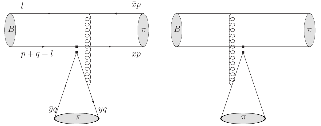
The hard spectator scattering diagrams, which are shown in LO in in fig. 2.2, contribute to . Through the soft momentum of the constituent quark of the -meson the hard collinear scale comes into play. This leads to the fact that in contrast to , which is completely governed by the scale , has to be evaluated at the hard-collinear scale. This leads to an enhancement of and makes the NLO corrections (i.e. ) of the hard spectator interaction diagrams more important. These corrections of are the topic of the present thesis. Hard spectator scattering corrections to the penguin diagram (third diagram of fig. 2.1) are beyond the scope of this thesis. The cancellation of the dependence on the renormalisation scale of this class of diagrams is completely independent of the “tree amplitude” i.e. the diagrams of fig. 2.2 and higher order corrections. For phenomenological applications, however, they should be taken into account.
2.2 Notation and basic formulas
2.2.1 Kinematics
For the process we will assign the momenta and to the pions which fulfil the condition
| (2.2) |
This is the leading power approximation in as we count the mass of the pion as . Let us define two Lorentz vectors , by:
| (2.3) |
In the rest frame of the decaying meson can be defined to be in the direction of and to be in the direction of . Light cone coordinates for the Lorentz vector are defined by:
| (2.4) |
So one can decompose into:
| (2.5) |
such that
| (2.6) |
We denote the mass of the -meson with and the mass of the -quark with . The difference such that we cannot distinguish those masses in leading power. However setting
| (2.7) |
in Feynman integrals might lead to additional infrared divergences. So we have to perform the integral before we can make the substitution (2.7) unless we are sure that we do not produce infrared divergences. If we calculate Feynman integrals, it is convenient to set
| (2.8) |
such that . The dependence on can be reconstructed by giving the correct mass dimension to the physical quantities.
2.2.2 Colour factors
In our calculations we will use the following three colour factors, which arise from the algebra:
| (2.9) |
where is the number of colours.
2.2.3 Meson wave functions
The pion light cone distribution amplitude is defined by
| (2.10) |
The ellipsis stands for the Wilson line
| (2.11) |
which makes (2.10) gauge invariant. For the definition of the -meson wave function we need the special kinematics of the process. Following [9] let us define
| (2.12) |
In the calculation of matrix elements we get terms like:
| (2.13) |
We will only consider the case that the dependence of the amplitude on is like this:
| (2.14) |
In this case we can use the -meson wave function on the light cone which is given by [9]:
| (2.15) | |||||
where
| (2.16) |
It is now straight forward to write down the momentum projector of the -meson:
| (2.17) | |||||
At this point we give the following definitions
| (2.18) | |||||
| (2.19) |
2.2.4 Effective weak Hamiltonian
The effective weak Hamiltonian which leads to is given by [18]:
| (2.20) |
where and
| (2.21) | |||||
| (2.22) | |||||
| (2.23) | |||||
| (2.24) | |||||
| (2.25) | |||||
| (2.26) | |||||
| (2.27) |
Explicit expressions for the short-distance coefficients can be obtained from [18]. The decay amplitude of is given by
| (2.28) |
For later convenience we define
| (2.29) |
where () belongs to the first (second) term of (2.1). Because and contain different hadronic quantities, the renormalisation scale dependence of both of them has to vanish separately. So we can set their scales to different values and . As in there occurs only the mass scale we can set . In there occurs also the hard-collinear scale . As we will see this scale is an appropriate choice for .
In order to separate the QCD effects from the weak physics we write the matrix elements of the effective weak Hamiltonian in the following factorised form [10]:
| (2.30) |
where
| (2.31) |
Note that in contrast to [10] the electroweak corrections to the effective weak Hamiltonian are not included in the above equations as in the case of they can be safely neglected.

stands for the contributions of the annihilation topologies, which are shown in fig. 2.3. These contributions do not occur in leading power and cannot be calculated in a model independent way in the framework of QCD factorization. For the exact definition of I refer to [10]. The matrix elements of the operators are defined to be or corresponding to the flavour structure of the -mesons. The penguin contractions that are shown in the third diagram of fig. 2.1 and the contributions of the operators - are by definition contained in the amplitudes -. As we take in the present thesis only the “tree amplitude” (fig. 2.2) into account, we only calculate corrections to the amplitudes and .
The decay amplitudes of can be written in terms of as follows [10]:
| (2.32) |
where
and
| (2.33) |
For the LO and NLO results of the I refer to [10].
The annihilation contributions are parametrised in the following form [10]:
| (2.34) |
where
| (2.35) |
The parameters can be further parametrised by the Wilson coefficients occurring in (2.20) and purely hadronic quantities:
| (2.36) |
where the quantities are given by [10]:
| (2.37) |
Here is defined as in (2.33) and parametrises an integral that is divergent because of endpoint singularities. In section 4.4.2 I will give an estimate of for numerical calculations.
2.3 Hard spectator interactions at LO
The leading order of the hard spectator interactions which start at is shown in fig. 2.2. The hard spectator scattering kernel , which does not depend on the wave functions, can be obtained by calculating the transition matrix element between free external quarks, to which we assign the momenta shown in fig. 2.2. The variables are the arguments of , which arise from the projection on the pion wave function (2.10). In the sense of power counting we count all components of of , while the components of and are or exactly zero. We define the following quantities
| (2.38) |
We will see that in the end the dependence on vanishes in leading power such that we can use (2.17).
We consider the three cases , and . In the case, that the external quarks come with the flavour content of , the LO hard spectator amplitude for the effective operator reads:
| (2.39) | |||||
where the quark antiquark states in the input and output channels of the matrix element form colour singlets. The subscript “spect.” means that only diagrams with a hard spectator interaction are taken into account. The amplitude of vanishes to this order in . In the case of we get the tree amplitude from the matrix element of . The case does not need to be considered separately, because from isospin symmetry follows [19, 10]:
| (2.40) |
On the other hand the full amplitude is the convolution of with the wave functions, given by (2.1). To extract from (2.39) we need the wave functions with the same external states we have used in (2.39), i.e. we have to calculate the matrix elements (2.10) and (2.12), where the pion or -meson states are replaced by free external quark states. To the order we get
| (2.41) | |||||
By using
| (2.42) |
we finally obtain:
| (2.43) | |||||
It should be noted that only the first summand of the above equation contributes after performing the Dirac trace in four dimensions. The second summand is evanescent. This will be important, when we will calculate the NLO corrections of the wave functions (see section 3.3).
If we plug the hadronic wave functions defined by (2.10) and (2.17) into (2.42) i.e. we calculate the matrix element (2.39) between meson states instead of free quark states, we get for the LO amplitude 11 1 At this point I want to apologise to the reader because of a mismatch in my notation: is used for the matrix elements of the effective Operators between both free external quarks and hadronic meson states. It should become clear from the context what is actually meant.:
| (2.44) |
Following (2.1) and the conventions of [13] we write our amplitude in the form:
| (2.45) |
where in the case of we define
| (2.46) |
and in the case we define
| (2.47) |
Because we use the NDR-scheme which preserves Fierz transformations for and , has the same form for both decay channels. From (2.44) and (2.45) we get:
| (2.48) |
According to [10] the contribution of (2.44) to and (see (2.31)) is given by:
| (2.49) |
where
| (2.50) |
and the label II in (2.49) denotes the contribution to as defined in (2.29).
2.4 Calculation techniques for Feynman integrals
2.4.1 Integration by parts method
Integration by parts (IBP) identities were introduced in [20, 21]. An algorithm to reduce Feynman integrals by IBP-identities to master integrals is very well described in [22]. So I will only show the basic principles. Because the topic of my thesis is a one-loop calculation I will restrict to the one-loop case, the generalisation to multi loop is straight forward.
The most general form22 2 Tensor integrals which contain expressions like in the numerator can be reduced to scalar integrals as described in [23] of a one-loop Feynman integral is
| (2.51) |
where , and are the momenta which appear in the internal propagator lines. Without loss of generality we can assume that there is no in the numerator as we can make the replacement
| (2.52) |
Because of our special kinematics we have only three linearly independent momenta , so all of the momenta are linear combinations of . This will simplify the reduction of the Feynman integrals. We will define
| (2.53) |
to be a basis of where and .
Following [23] we can reduce (2.51) by performing algebraic transformations on the integrands, which are defined in the following three rules:
Rule 1.
Consider the case that there exist such that
| (2.54) |
Now we can make the following simplification ():
| (2.55) | |||||
and the scalar product has disappeared from the numerator. If (2.54) cannot be fulfilled we use the identity
| (2.56) |
to reduce our set of integrals further. This identity does not reduce the total number of scalar products in the numerator but the number of different scalar products.
Rule 2.
For scalar products of the form we make the replacement
| (2.57) |
Rule 3.
Now consider the case that our integrand is of the form
| (2.58) |
where . In that case we use the following rule: Choose a set which is a basis of . Choose such that forms a basis of . Complete to a basis of by adding elements of to . Then write as a linear combination of this new basis and apply (if possible) (2.55), (2.56) or (2.57) respectively.
For the following identities which are called integration by parts or IBP identities we will use the fact that in dimensional regularisation an integral over a total derivative with respect to the loop momentum vanishes. Using the definitions of (2.51) we get two further rules:
Rule 4.
| (2.59) | |||||
where and .
Another identity is:
Rule 5.
| (2.60) | |||||
where .
For the IBP identities (2.59) and (2.60) we have used the translation invariance of the dimensional regularised integral. We get another class of identities if we use the invariance under Lorentz transformations. From equation (2.9) of [24] we get
| (2.61) | |||||
We choose . By multiplying of (2.61) with we get
Rule 6.
An implementation in Mathematica of the IBP identities can be found in appendix A.
2.4.2 Calculation of Feynman diagrams with differential equations
In this section I will discuss the extraction of subleading powers of Feynman integrals with the method of differential equations [25, 26, 24]. This method will prove to be easy to implement in a computer algebra system. The idea to obtain the analytic expansion of Feynman integrals by tracing them back to differential equations has first been proposed in [25]. This method, which is demonstrated in [25] by the one-loop two-point integral and in [26] by the two-loop sunrise diagram, uses differential equations with respect to the small or large parameter, in which the integral has to be expanded.
In contrast to [25, 26] I will discuss the case that setting the small parameter to zero gives rise to new divergences. In this case the initial condition is not given by the differential equation itself and also cannot be obtained by calculation of the simpler integral that is defined by setting the expansion parameter to zero. It is not possible to give a general proof, but it seems to be a rule, that one needs the leading power as a “boundary condition”, which can be calculated by the method of regions [27, 28, 29, 30]. The subleading powers can be obtained from the differential equation. In the present section I will discuss which conditions the differential equation has to fulfil in order for this to work.
Description of the method
We start with a (scalar) integral of the form
| (2.63) |
where the propagators are of the form . We assume that there is only one mass hierarchy, i.e. there are two masses such that all of the momenta and masses and are of or of . We expand (2.63) in by replacing all small momenta and masses by and expand in . After the expansion the bookkeeping parameter can be set to .
We obtain a differential equation for by differentiating the integrand in (2.63) with respect to . This gives rise to new Feynman integrals with propagators of the form and scalar products in the numerator. Those Feynman integrals, however, can be reduced to the original integral and to simpler integrals (i.e. integrals that contain less propagators in the denominator) by using integration by parts identities.
Finally we obtain for (2.63) a differential equation of the form
| (2.64) |
where contains only rational functions of and can be expressed by Feynman integrals with a reduced number of propagators. It is easy to see that and are unique if and only if and the integrals contained in are master integrals with respect to IBP-identities, i.e. they cannot be reduced to simpler integrals by IBP-identities. If is divergent in , , and have to be expanded in :
| (2.65) |
Plugging (2.65) into (2.64) gives a system of differential equations for , similar to (2.64). In the next paragraph we will consider an example for this case.
First let us assume that and have the following asymptotic behaviour in :
| (2.66) |
i.e. starts at , and we allow that starts at a negative power of . We count as so the may depend on . This dependence, however, has to be such that
| (2.67) |
The condition (2.67) is fulfilled, if the are of the form of a finite sum
| (2.68) |
The limit however can spoil the expansion (2.66). E.g. so the condition (2.67) is not fulfilled, which is due to the fact that we must not change the order of the limits and .
Further we assume that also starts at
| (2.69) |
and plug this into (2.64) such that we obtain an equation which gives recursively:
| (2.70) |
I want to stress that, because starts at , (2.70) is a recurrence relation, i.e. does not mix into if . As the integral is only well defined if , we need the leading power as “boundary condition” and (2.70) will give us all the higher powers in . It is easy to implement (2.70) in a computer algebra system, because we just need the integration of polynomials and finite powers of logarithms.
A modification is needed if starts at i.e.
| (2.71) |
By replacing we obtain the differential equation
| (2.72) |
which is similar to (2.64) and leads to
| (2.73) |
which is valid for . So, if starts at , the subleading powers result from the leading power.
Examples
We start with a pedagogic example:
Example 2.4.1.
| (2.74) |
where . The exact expression for this integral is given by:
| (2.75) |
We see that diverges for . As described e.g. in [30] we can obtain the leading power by expanding the integrand in the regions and . This leads in the first region to
| (2.76) |
and in the second region to
| (2.77) |
such that we finally obtain
| (2.78) |
This is the result we obtain from the leading power of (2.75). We write the derivative of with respect to in the following form:
| (2.79) |
We obtained the right hand side of (2.79) by decomposing into partial fractions. Of course this decomposition is not unique which is due to the fact that itself is not a master integral but can be further simplified by partial fractioning. From (2.79) and (2.64) we get:
| (2.80) |
such that the coefficients in the expansion in according to (2.66) do not depend on the power label :
| (2.81) |
We obtain for the recurrence relation (2.70):
| (2.82) |
Using the initial value (2.78) it is easy to prove by induction
| (2.83) |
This result coincides with (2.75).
The first nontrivial example, we want to consider, is the following three-point integral:
Example 2.4.2.
| (2.84) |
Here and are collinear Lorentz vectors, which fulfil and , is a real number between and and is a Lorentz vector with and . Furthermore we define
| (2.85) |
We expand in , so we make the replacement and differentiate with respect to . The integral is not divergent in such that we obtain a differential equation of the form (2.64) where the Taylor series of starts at as in (2.66). In only two-point integrals occur, which are easy to calculate. I do not want to give the explicit expressions for and because they are complicated, their exact form is not needed to understand this example and they can be handled by a computer algebra system. Because the leading power of is of , (2.70) gives all of the subleading powers.
We obtain the leading power as follows: First we have to identify the regions, which contribute at leading power. If we decompose into
| (2.86) |
we note that the only regions, which remain at leading power, are the hard region and the hard-collinear region
| (2.87) |
The soft region leads at leading power to a scaleless integral, which vanishes in dimensional regularisation. In the hard region we expand the integrand to
| (2.88) |
By introducing a convenient Feynman parametrisation we obtain for the -dimensional integral over (2.88):
| (2.89) |
In the hard-collinear region we expand the integrand to
| (2.90) |
The integral over (2.90) gives:
| (2.91) |
So adding (2.89) and (2.91) together we get the leading power of (2.84):
| (2.92) |
By plugging (2.92) into (2.70) we obtain at :
| (2.93) |
Now we want to consider the following four-point integral
Example 2.4.3.
| (2.94) |
where we used the same variables, which were introduced in (2.84). This example is very special, because in this case our method will allow us to obtain not only the subleading but also the leading power in . is divergent in such that we obtain after the expansion (2.65) a system of differential equations of the following form:
| (2.95) |
It turns out that in our example takes the simple form
| (2.96) |
such that analogously to (2.72) we can transform (2.95) into
| (2.97) |
This system of differential equations can easily be integrated to:
| (2.98) |
where the superscript denotes the order in as in (2.66) and (2.69). Both and start at . Because (2.98) is valid for , it gives us the leading power expression, which reads:
| (2.99) |
where as in the example above. The exact expression for (2.94) can be obtained from [31]. Thereby (2.99) can be tested.
A simplification for the calculation of the leading power
In the last paragraph I want to return to Example 2.4.2. I will show how we can use differential equations to prove that the integral (2.84) depends in leading power only on the soft kinematical variable and not on . We need derivatives of the integral with respect to and , which we have to express through derivatives with respect to . These derivatives can be applied directly to the integrand, whose dependence on is obvious. We start from the following identities:
| (2.100) | |||||
which lead to
| (2.101) |
where we have set in (2.101). Using (2.101) we can show that in leading power (2.84) depends only on and not on . So we can simplify the calculation of the leading power by making the replacement . The proof goes as follows: From (2.69) we see that the statement “ does not depend on ” is equivalent to
| (2.102) |
Using the first equation of (2.101) we get
| (2.103) |
Because we know (e.g. from power counting) that starts at , (2.102) is proven.
Chapter 3 Calculation of the NLO
3.1 Notation
3.1.1 Dirac structure
In this thesis I used the NDR scheme [32] such that -matrices are anticommuting. We get for the matrix elements of and Dirac structures of the following type:
| (3.1) |
where are - or -quarks. To avoid to specify the flavour, which depends on the decay mode, I introduce for (3.1) the following short notation:
| (3.2) |
The equations of motion lead to:
| (3.3) |
3.1.2 Imaginary part of the propagators
Unless otherwise stated propagators in Feynman integrals always contain an term where and we take the limit after the integration. For example an integral of the form
is just an abbreviation for
If the propagator does not contain the integration momentum quadratically, the will always be given explicitly.
3.2 Evaluation of the Feynman diagrams


The diagrams that contribute to at NLO are listed in fig. 3.1 - 3.7. Fig. 3.1 shows the gluon self energy. This is a subclass of diagrams which factorizes separately. After adding the counter term for the gluon propagator the contribution to is:
| (3.4) | |||||
For (3.4) we have set the number of active quark flavours to and set the mass of the -, -, - and -quark to zero.
For the rest of this section I will consider only those diagrams, for which the calculation of Feynman integrals is not straight forward. I will only show how those Feynman integrals can be calculated in leading power. For higher powers I refer to the methods shown in section 2.4.2. It is important to note, that though for the evaluation of the Feynman integrals arguments depending on power counting have been used, all of the integrals occuring in this section have been tested by methods that do not depend on power counting.
The first class of diagrams with non trivial Feynman integrals are the diagrams in fig. 3.3. The two diagrams from fig. 3.3(a) read
| (3.5) |
| (3.6) |
The denominators of (3.5) and (3.6) are identical up to the substitution . So the Feynman integrals we have to calculate are the same. We can reduce our five-point integrals to four-point integrals by expanding the denominator of the integrand into partial fractions
| (3.7) | |||||
Only the first two summands of the right hand side of this equation give leading power contributions to aII1 and aII2:
| (3.8) | |||||
| (3.9) |
The third one
| (3.10) |
gives only a leading power contribution in the hard-collinear region
| (3.11) |
and the soft region
| (3.12) |
where we introduced the counting and set . In both regions the leading power of the numerators of aII1 and aII2 vanishes because of equations of motion. The fourth summand of (3.7)
| (3.13) |
does not give a leading power contribution at all.
The topologies and are exactly the denominators of the Feynman integrals of the last four diagrams of fig. 3.3:
| aII3 | (3.14) | ||||
| aII4 | (3.15) | ||||
| aII5 | (3.16) | ||||
| aII6 | (3.17) | ||||
where the Feynman diagrams are given in the same order as they occur in fig. 3.3. So we have reduced all the Feynman integrals of fig. 3.3 to the topologies and . Regarding we need the scalar integral
| (3.18) |
By following the procedure of [23] the tensor integrals , and can be reduced to (3.18) and to the two-point master integrals that are listed in appendix B.1. The leading power of (3.18) gets only contributions from the region where is soft i.e. all components of are of . In this region we can expand the integrand of (3.18) to
| (3.19) |
Now we can obtain the leading power of (3.18) by integrating (3.19) over all momenta because there is no other region, which gives a leading power contribution, besides where is soft. The integration of (3.19) can be easily performed by using the following Feynman parametrisation [33]:
| (3.20) |
Finally we obtain for the leading power of (3.18)
| (3.21) |
Regarding the topology we need the tensor integrals , and . This topology can be reduced to two-point master integrals and to the four-point master integral
| (3.22) |
In order to calculate this integral we decompose into
| (3.23) | |||||
where only the integral over the first summand of (3.23) gives a leading power contribution. This integration is straight forward if one uses the Feynman parametrisation (3.20).
Finally we get the leading power of (3.22):
| (3.24) |
Actually it turns out that the sum of the diagrams in fig. 3.3 vanishes in leading power.
The diagrams of fig. 3.4 are straight forward to calculate. It is easy to see that in leading power does not occur within a loop integral. So there are only two linearly independent momenta in the Feynman integrals, which, using similar relations like (3.7) and IBP identities, can be reduced to the master integrals that are listed in appendix B.1.
The diagrams of fig. 3.5(a),(b) are easy to calculate, because they contain only three-point integrals. The next two (fig. 3.5(c)) are given by
| (3.25) | |||||
| (3.26) | |||||
By expanding the denominator of (3.25) or (3.26) into partial fractions we get:
| (3.27) | |||||
where we get leading power contributions only from:
| (3.28) | |||||
| (3.29) | |||||
| (3.30) |
The leading power of (3.28) can be taken from (3.21). We obtain the leading power of (3.29) by making the replacement . Alternatively we can use (B.18) in appendix B.2 and take the leading power afterwards. For (3.30) we obtain the leading power by making the replacement . In contrast to (3.29) this replacement is not so obvious and to calculate this integral exactly is very involved. However we can start with the value, we obtained by this prescription, and show afterwards by solving a partial differential equation that it is correct. We define
| (3.31) |
and derive two differential equations by deriving with respect to and to . As a boundary condition for our differential equations we calculate at the point and . This can be done by decomposing into partial fractions and using IBP identities. We use the fact that the limits and do not lead to extra divergences in and in . So we can solve our differential equations order by order in and . Defining
| (3.32) |
and using the fact that we only need the leading power in we obtain differential equations of the form
| (3.33) |
The coefficients , , , and are straight forward to calculate using IBP identities and the master integrals are given in appendix B.1. It turns out that the leading power integral we obtained by the prescription fulfils our boundary condition for and as well as the set of differential equations (3.33).
The sum of the following two diagrams (fig. 3.5(d)) is
| (3.34) | |||||
As in the previous case the denominator can be decomposed into partial fractions and the remaining four-point master integrals can be calculated in leading power by the replacement . Alternatively we can use the explicit formulas for four-point integrals given in [31] and derive the leading power (and higher powers if necessary) afterwards. This is what I have done in order to get an independent test of my master integrals.
The last two diagrams of this class (fig. 3.5(e)) are given by
| (3.35) | |||||
As in the case before we obtain the leading power of the four-point master integrals by the replacement or by using the formulas in [31]. The denominator of (3.35) however cannot by decomposed into partial fractions. So we additionally need the five-point master integral given in appendix B.3.
Regarding the diagrams in fig. 3.6 there do not occur any subtleties we have not yet considered in the paragraph above. So we directly switch to the non-abelian diagrams in fig. 3.7. The first four (fig. 3.7(a),(b)) do not lead to any problems because they contain only three-point integrals. The diagrams in fig. 3.7(c) are given by
| (3.36) | |||||
The four-point integral we have to solve is nearly the same as (2.94) of example 2.4.3. We can reduce this integral to a solution of a differential equation and get in this way every power in .
The last diagrams we will consider are those from fig. 3.7(d). In leading power they read:
| (3.37) | |||||
The scalar master integral
| (3.38) |
can be calculated in leading power by setting i.e. we make the replacement . This can be seen as follows: Counting soft momenta as and hard momenta as (remember ) the regions of space where (3.38) gives a leading power contribution are
In these regions occurs only in the combination . So we can make the replacement . Those people who do not believe these arguments are invited to use the exact expression (B.17) for the four-point integral with one massive propagator line, which is given in appendix B.2. After taking the leading power it can easily be seen that we get the same result as by just making the replacement .
The diagrams which contribute to are those of fig. 3.3 and fig. 3.4. The other diagrams drop out because their colour trace is zero. As in the case of the diagrams of fig. 3.3 cancel each other in leading power. The remaining diagrams are easy to calculate because their Feynman integrals are the same as in the case of .
3.3 Wave function contributions
3.3.1 General remarks
It has already been demonstrated in section 2.3 how in principle we can extract the scattering kernel of (2.1) from the amplitude if we know the wave functions. does not depend on the hadronic physics and on the form of the wave function and in particular, so we can get by calculating the matrix elements of the effective operators between free quark states carrying the momenta shown in fig. 2.2 on page 2.2. Because we calculate in NLO we need unlike as in section 2.3 the wave functions up to NLO. Let us write the second term of (2.1) in the following formal way:
| (3.39) |
All of the objects arising in (3.39) have their perturbative series in , so (3.39) becomes
| (3.40) | |||||
where the superscript denotes the order in 11 1 Please note that the hard spectator scattering kernel starts at . So we call the LO and the NLO.. In order to get we have to calculate , and for our final states. Then is given by
| (3.41) | |||||
At this point a subtlety occurs. Let us have a closer look to the factorization formula (2.1). By calculating the first order in of the partonic form factor , which is defined by free quark states instead of hadronic external states, we see that it can be written in the form
| (3.42) |
But is no part of . So we have to modify (3.41) insofar as we have to subtract the right hand side of (3.42) from the right hand side of (3.41):
| (3.43) | |||||
In (3.43) we did not include the term , because it is obviously identical with the diagrams where the gluons do not interact with the emitted pion (e.g. those of fig. 3.8).

Those diagrams where not considered in the last section. So we do not have to consider them here.
The wave functions for free external quark states are given at LO by (2.41). At NLO there exist three possible contractions: The two external quark states can be connected by a gluon propagator or one of the external quarks can be connected to the eikonal Wilson line of the wave function (fig. 3.9).

The diagrams of fig. 3.9(a),(b) and (c) give of the “pion wave function for free quarks”, i.e. we have replaced the pion final state in (2.10) by the free quark state . The Fourier transformed wave function is defined analogously to (2.41). For the diagrams in fig. 3.9 (a), (b) and (c) respectively we get:
3.3.2 Evanescent operators
At NLO the convolution of the wave functions with the tree level kernel gives rise to new Dirac structures, which, however, can in four dimensions be reduced to the tree level Dirac structures. So we obtain the tree level Dirac structures plus further evanescent structures, which vanish for but give finite contributions if they are multiplied by UV-poles. We define our renormalisation scheme such that we subtract the UV-poles and these finite parts of the evanescent structures.
The tree level kernel (2.43) contains two Dirac structures where the second one is evanescent (after the the projection on the wave functions). We write in the following form (that must not be mixed up with the notation (3.2)):
| (3.45) |
where the symbol stands for the “wrong contraction” of the Dirac indices i.e. the Dirac indices are given by
| (3.46) |
as in (2.43). The “right contraction” is defined by the symbol i.e. writing the Dirac indices explicitly
| (3.47) |
In the wrong and the right contraction are related by Fierz transformations. It is convenient and commonly used to define the renormalised wave functions in terms of the right contraction, i.e. to define by renormalising the operator instead of . This is why we define our renormalisation scheme such that only the UV-finite part of the right contraction operators remains: Using the notation of (3.45) – (3.47) we define the following operators:
| (3.48) | |||||
| (3.49) | |||||
| (3.50) |
The matrix elements of these operators are defined analogously to (2.42):
| (3.51) |
Note that is just the convolution of the tree level kernel (3.45) with the wave functions. Furthermore by using Fierz identities it is easy to prove that we have in four dimensions
| (3.52) | |||||
| (3.53) |
So we define the following evanescent operators:
| (3.54) | |||||
| (3.55) | |||||
| (3.56) | |||||
| (3.57) |
where we have defined and for later convenience. Using those operator definitions we define our renormalisation scheme such that we subtract the UV-pole of and the finite parts of i.e. terms of the form , where is an arbitrary evanescent structure. It is important to note that we do not subtract IR-poles, because they depend not only on the operator but also on the external states the operator is sandwiched in between. They have to vanish in (3.43) such that the hard scattering kernel is finite. Finally we obtain the same result as if we had regularised the IR-divergences by small quark and gluon masses because the evanescent structures vanish in .
In the next step we will calculate the convolution integral of with the NLO wave functions given by (), i.e. we have to calculate the renormalised matrix elements of at NLO.
3.3.3 Wave function of the emitted pion
First we consider the renormalisation of the emitted pion wave function: Because the contribution of the wave functions and does not change the Dirac structure of the operators, we do not need to consider evanescent operators when we calculate the diagrams of fig. 3.9(a),(b). So for the emitted pion wave function these diagrams give after renormalisation:
| (3.58) |
where the LO matrix elements can be obtained from (2.39). Note that we kept the IR-pole times the evanescent matrix element . This is needed for consistency because we also kept similar terms in the QCD-calculation of . Furthermore it allows us to show that all IR-divergences vanish.
The diagram in fig. 3.9(c) mixes different Dirac structures. So we have to include evanescent operators in the renormalisation. In the case of the emitted pion wave function the operator does not mix under renormalisation with the evanescent operator (3.54). We obtain for the renormalised matrix element:
| (3.59) |
The matrix element of however has an overlap with :
| (3.60) |
The renormalisation prescription tells us to subtract the UV-pole and the UV-finite part of . So we obtain after renormalisation:
| (3.61) |
Note that the evanescent operator leads to a finite term , which we would have missed if we had just dropped the evanescent operators.
3.3.4 Wave function of the recoiled pion
In the next step we consider the NLO contribution of the recoiled pion wave function. As in the case of the emitted pion the diagrams fig. 3.9(a),(b) do not lead to a mixing between the operators. Therefore we get:
| (3.62) |
Other than in the case of the emitted pion the operators and mix the spinors of the recoiled pion and the -meson. Therefore we have to work in the operator basis of and the evanescent operators and define our renormalisation scheme such that the finite parts of the matrix elements of the evanescent operators vanish. The diagram fig. 3.9(c) contributes to the matrix element of the renormalised operator :
| (3.63) |
In the case of the evanescent operators we keep the IR-pole:
| (3.64) | |||||
| (3.65) |
At the end of the day we obtain a contribution from diagram fig. 3.9(c):
| (3.66) |
The very complicated but also very explicit form, in which the above equation was given, is rather convenient, because on the QCD side the diagrams in fig. 3.5(e) on page 3.5 come with the same Dirac structure and cancel the IR-pole of (3.66).
3.3.5 Wave function of the -meson
The corrections of the wave function of the -meson are given by the second row of fig. 3.9. For the diagrams (d), (e) and (f) respectively they read:
| (3.67) | |||||
In the case of the -meson only the diagrams in fig. 3.9(d),(e) give rise to UV-poles. Those diagrams however do not lead to a mixing of and the evanescent operators and we do not have to deal with evanescent operators.
First let’s have a look at the convolution integral which belongs to the diagram in fig. 3.9(f) 22 2 In order not to confuse the reader I stress that the symbols , in this and the following equations are meant in terms of (3.2) and not of (3.46).:
| (3.68) | |||||

In leading power (3.68) is identical to the contribution of the two diagrams shown in fig. 3.10, which is given by:
| (3.69) |
In (3.69) the leading power comes from the region where is soft. In this region of space the integrand gets the form of the integrand in (3.68), so both contributions cancel. As we did not include the diagrams of fig. 3.10 in the last section we can skip the contribution of (3.68) here.
The remaining contributions are the diagrams in fig. 3.9(d) and (e). Together they read:
| (3.70) | |||||
3.3.6 Form factor contribution

Finally we have to calculate the contribution of (3.42). It is given by
| (3.71) | |||||
The form factor is the correction of the matrix element
| (3.72) |
where and are the spinors with the flavour quantum numbers of the emitted pion and is given by [10]:
| (3.73) | |||||
We get by evaluating the diagrams in fig. 3.11. Using the notation of (3.2) we finally obtain:
| (3.74) | |||||
Chapter 4 NLO results
4.1 Analytical results for and
After the analysis of the last chapter we finally obtain the results for the hard spectator scattering kernels which are defined by (2.45). Those expressions appear in convolution integrals with wave functions, where , and are the integration variables as defined in (2.45). The ultraviolet divergences are renormalised in the -scheme. The infrared divergences drop out after subtracting the wave function contributions from the amplitude. The infrared finiteness together with the finiteness of the convolution integrals ensures that the framework of QCD-factorization works at this order in .
The explicit contributions for read (see next page):
| (4.1) | |||||
| (4.2) | |||||
| (4.3) | |||||
| (4.4) | |||||
The corrections of the hard spectator interactions have already been calculated in [13, 14]. However both of these calculations have been performed in the framework of SCET, while my result is a pure QCD calculation. In order to compare (4.1)-(4.4) to [13, 14] we have to take into account the definition of . The SCET calculation naturally uses the , defined by the HQET field for the -meson, while I define by QCD-fields. Those two definitions differ at , which has been discussed in appendix C. The difference in the logarithmic moments of the -meson wave function does not play a role, because these moments occur first at NLO. Using (C.14) I figured out with the help of a computer algebra system, that (4.1)-(4.4) reproduce the results of [13, 14].
The main difference between the present QCD calculation and the framework of SCET is the way how to make the expansion in . While in the QCD calculation this expansion takes place at the level of the amplitude and of Feynman integrals, in SCET the Lagrangian is expanded in powers of . This leads to the fact that the structure of the calculation of [13, 14] is completely different from the present calculation such that comparing intermediate results like single Feynman diagrams is not possible. So it is allowed to state that the analytical coincidence of the present result with the results published before gives more independent test of [13, 14] than than a SCET calculation could provide.
4.2 Scale dependence
It is instructive to have a closer look to the scale dependence of (4.1)-(4.4). As stated in section 2.2.4 the scale dependence of vanishes. In our case we can prove this up to i.e.
| (4.5) |
We need the scale dependence of the following quantities, which I took from [18]:
| (4.6) | |||||
| (4.7) | |||||
| (4.8) |
where and the number of active flavours. Regarding the wave functions we need the scale dependence of their convolution integrals with the LO kernels:
| (4.9) | |||||
| (4.10) |
(4.9) can be obtained using the renormalisation group equation (RGE) for light-cone distribution amplitudes, which can be found in [9, 34]. We get (4.10) from [35], where the RGE for the -meson light-cone wave function, defined in the framework of HQET, is given. We get the RGE for the pure QCD defined wave function by matching the nonlocal heavy to light current with QCD. The matching coefficient is given in Appendix C.
4.3 Convolution integrals and factorizability
By looking at the hard scattering kernels of (4.1)-(4.4) it is not obvious that there remain no singularities in the convolution integrals over wave functions (2.45). It is however possible to perform the integration analytically, which proves the factorizabilty.
Regarding the -meson wave function we will obtain the result in terms of the quantities and , which are defined in (2.18) and (2.19). The -meson wave function is given in terms of Gegenbauer polynomials:
| (4.12) |
Because of the symmetry properties of the pion we set , furthermore we neglect for . So we need only the second Gegenbauer polynomial which is given by:
| (4.13) |
Using (2.45) we get for the NLO of :
| (4.14) |
and
| (4.15) |
The finiteness of the above equations proves factorization of the hard spectator interactions at NLO.
4.4 Numerical analysis
4.4.1 Input parameters
| CKM-parameters | ||||||||||||||
| ||||||||||||||
| Parameters of the -meson | ||||||||||||||
| ||||||||||||||
| Parameters of the -meson | ||||||||||||||
| ||||||||||||||
| Quark and W-boson masses | ||||||||||||||
| ||||||||||||||
| Coupling constants | ||||||||||||||
|
For my numerical analysis I use the parameters given in table 4.1. The decay constant and the ratio have been obtained by QCD sum rules in [36] and [37] respectively. The logarithmic moments and where calculated in [13] using model light-cone wave functions for the -meson [44, 45, 46, 47]. For the form factor I use the value from [40], which has been obtained by QCD sum rules. This value is consistent with quenched and recent unquenched lattice calculations [38, 39]. The first Gegenbauer moment of the pion wave function is zero due to G-parity while the second moment has been obtained by lattice simulations [41, 42].
4.4.2 Power suppressed contributions
In our numerical analysis we include two contributions which are suppressed in leading power but numerically enhanced: The twist-3 contributions and the annihilation topologies.
The twist-3 contributions come from the twist-3 contributions of the pion wave functions and are suppressed by the factor
(see (2.33)), which is formally of but numerically about . These contributions modify the hard spectator scattering function (2.50) to [10]
| (4.18) |
where is parametrised by:
| (4.19) |
with
| (4.20) |
For numerical calculations we set
| (4.21) |
4.4.3 Amplitudes and
The amplitudes and are defined in (2.31). Their hard scattering parts and , i.e. the parts of and , which contribute to (see (2.29)), are plotted in fig. 4.1 as functions of the renormalisation scale . The strong dependence on of the real part of LO is reduced at NLO. Taking the twist-3 contributions into account does not increase the -dependence too much. The imaginary part, which occurs first at NLO, is strongly dependent on the renormalisation scale. An appropriate choice for the scale of the hard scattering amplitude is the hard collinear scale
| (4.24) |
In the following numerical calculations we will evaluate and at . The vertex corrections will be evaluated at
| (4.25) |
Using the parameters of table 4.1 we obtain
| (4.26) |
These equations are given in a form similar to (61) and (62) in [13]. The first number gives the tree contribution, the vertex corrections are indicated by the label , the twist-3 contributions, which come from the last part of (4.18), are labelled by tw3. The hard scattering part is separated into LO and NLO. The hadronic input parameters I used are slightly different from [13] and in contrast to [13] I evaluated all quantities, which belong to the hard scattering amplitude, at the hard collinear scale . This is why the values I get for and are different from [13].
The hard scattering amplitudes and together with their numerical errors read:
| (4.27) |
The first error comes from the error of the input parameters in table 4.1. The scale uncertainty is obtained by varying between 1GeV and 6GeV. The error labelled by tw3 gives the error of the twist-3 contribution, which is obtained by varying between 0 and 1 and between 0 and . Within the scale uncertainty (4.27) is compatible with [13].
It is important to remark that the result I obtained in QCD comes with formally large logarithms . In contrast to the SCET calculation of [13, 14] it is not possible to resum these logarithms by a pure QCD calculation. Without resummation, however, these logarithms might spoil perturbation theory. Regarding this fact it is the more important that the error arising from the scale uncertainty in (4.27) is small enough for perturbation theory to be valid.
4.4.4 Branching ratios
The dependence of the CP-averaged branching ratios on the hard collinear scale is shown in fig. 4.2. It is obvious that the NLO corrections reduce this dependence significantly.
From the parameter set in table 4.1 we obtain the following CP-averaged branching ratios
| (4.28) |
The origin of the errors are the uncertainties of the hadronic parameters and the CKM parameters, the scale dependence and the subleading power contributions, i.e. twist-3 and annihilation contributions. The error arising from the scale dependence was estimated by varying between 2GeV and 8GeV and between 1GeV and 6GeV. If we compare (4.28) to the experimental values [7]:
| (4.29) |
we note that is in good agreement with the data. This quantity is almost independent of . The other branching ratios, which come with large errors, depend strongly on . This dependence is shown in fig. 4.3. The light-grey band gives the uncertainty that is defined in the same way as the errors in (4.28), where different errors are added in quadrature. The solid inner line gives the central value. The experimental values are represented by the horizontal band, whereas the vertical band gives the value of . It is obvious that the errors of the branching fractions are too large for a reasonable determination of .
For and QCD-factorization is expected to work well, because at tree level Wilson coefficients occur in the so called colour allowed combination , while comes at tree level with such that subleading power corrections are expected to be more important. On the other hand there are big uncertainties in the parameters occurring in the combinations , and . In [48] and [13] these parameters were fitted by the experimental values (4.29) of and . Setting
| (4.30) |
leads to
| (4.31) |
This leads to the following branching ratios:
| (4.32) |
The uncertainties of the quantities that occurred in (4.30) and (4.31) have not been considered in the estimation of the errors in (4.32). The branching ratio obtained in (4.32) is compatible with the value obtained in [13]. Though it is too low, due to the theoretical and experimental errors it is compatible with (4.29).
There are two different sources of errors. On the one hand for errors that are due to uncertainties of input parameters and the renormalisation scale there is at least in principle no lower limit. On the other hand errors arising from subleading power corrections, i.e. twist-3 and annihilation contributions, cannot be reduced in the framework of QCD-factorization. Fig. 4.4 shows the branching fractions of and as functions of . The errors arising from subleading power contributions are represented by the dashed lines inside of the light-grey error band. While in the case of this remaining error might be small enough for non-trivial phenomenological statements about , in the case of there remains an error of about 30%.
Chapter 5 Conclusions
In the last decades physics has proven a promising field to determine parameters of the flavour sector with high precision. It is expected that in the next few years the angles and , which are directly connected to the complex phase of the CKM matrix, will be measured with an accuracy at the percent level. Furthermore the discovery of physics beyond the standard model will be possible.
On the theoretical side QCD factorization has turned out to be an appropriate tool to calculate decay modes from first principles, because it allows for systematic disentanglement of the perturbative physics and the non-perturbative physics. The present calculation showed that the hard spectator scattering amplitude factorizes up to and including , i.e. all infrared divergences cancel and there are no remaining endpoint singularities. The former point is obvious after the explicit calculation of and the latter point was shown by evaluating the convolution integral (2.1) analytically. The explicit expressions for the hard spectator scattering kernel (4.1)-(4.4) confirmed the result of [13, 14]. So they are also a confirmation that the leading power of the amplitudes can be obtained by performing the power expansion at the level of Feynman integrals rather than at the level of the QCD Lagrangian using an effective theory like SCET, which was done in [13, 14].
The main challenges in the evaluation of Feynman integrals, which were made possible with the help of tools like integration by parts identities and differential equation techniques, were due to the fact that the Feynman integrals came with up to five external legs and three independent rations of scales. Many steps in the calculations of section 3.2 might look like cookery. However I dare say calculating Feynman integrals is cookery.
One motivation to calculate the corrections of the hard spectator interactions separately is the fact, that the LO of this class of diagrams starts at such that in order to fix the scale we need the NLO correction. The numerical results of section 4.4.3 show that the NLO reduces the scale dependence significantly. This is even more important with respect to large logarithms that arise because of the fact that next to the -scale also the hard-collinear scale enters the hard spectator scattering amplitude. In contrast to the effective theory ansatz the QCD calculation of this work does not allow the resummation of these logarithms. This is why it is a crucial point, that the NLO is numerically important but small enough for perturbation theory to be valid.
Next to the scale dependence a main source of uncertainty is due to the fact that we do not know hadronic quantities well enough. This might be improved in the next few years by lattice calculations and even determination of the hadronic input parameters in experiment. Also a better control of power corrections would allow to obtain much more precise predictions from QCD factorization.
Finally it is important to note that the present calculation is not the complete order result as the contributions of penguin contractions and the effective penguin operators where not considered in this thesis. Actually they play a dominant role in the branching ratios of and CP asymmetries of and should be taken into account in phenomenological applications. While writing down this thesis the order of these contributions has been recently published in [49]. Also the corrections of were not part of this thesis. These contributions have been calculated in [11, 12].
So the calculation of the present thesis is a small but very important tessera in the mosaic of theoretical -physics.
Appendix A CAS implementation of IBP identities
A.1 User manual
This section will give an introduction how to use my Mathematica packages lorentz.m and ibp.m. These packages use the rules of section 2.4.1 and the algorithm of [22]. You can download these files from
http://www.theorie.physik.uni-muenchen.de/~pilipp
I assume that these files are located on your hard disk in the directory path. After you have started your Mathematica notebook with the two lines
   <<path/lorentz.m;
   <<path/ibp.m;
you have to set some variables. Because my program distinguishes between Lorentz vectors and scalars we have to define which variables are of the type vector. This is done with the function
AddMomenta[p1,...,pn]
which defines the variables p1,...,pn to be of the type vector. The function
RemMomenta[p1,...,pn]
removes the attribute vector from p1,...,pn and
ShowMomenta[]
gives list of all vector variables. Per default the variables p, q and l are defined to be vector variables.
The syntax of defining scalar products is the same as in Tracer [50]. The OnShell-command
OnShell[on,{p1,0},{p2,p3,m},...]
defines the scalar products and . By default there are the following definitions:
OnShell[on,{p,0},{q,0},{l,0},{p,q,1/2},{p,l,xi/2},{q,l,theta/2}]
To undo the onshell definition use the flag off instead of on.
An integral of the form (2.51) contains the set of momenta , which are in general linear combinations of basis momenta e.g. where the basis momenta are . To tell Mathematica which variables are the basis momenta we have to define the variable MomBasis. In our example we set:
After this definition the function
has to be called to tell Mathematica that are the momenta which appear in the Feynman integrals. In the above example:
Feynman integrals are represented by the function FInt. This function will be simplified applying rule 1, 2 and rule 3 of section 2.4.1. After the call of the function the momentum is represented by the position at which it appears in the argument list. So the integral (2.51) is represented by
Because most integrals do not have propagators of the form , the second argument of FInt can be dropped such that
represents the integral
For example: We want to represent the integral
| (A.1) |
After the above call of ExternalMomenta[0,p,p+y*q] the momenta 0, p, p+y*q are represented by the numbers 1, 2 and 3 respectively. So (A.1) is represented by
which is transformed into
because rule 1 and rule 3 are applied and scaleless integrals vanish in dimensional regularisation.
The identities from rule 4 to rule 6 are created by the function IBP. This function takes three or five arguments and is called by
or
which is a shortcut for
The first two arguments of IBP Denom1 and Denom2 are lists that take the form and respectively and describe the topology i.e. they tell Mathematica to create identities of integrals which contain the propagators and respectively. The powers and to which the propagators and have to appear, are given by the next two arguments la1 and la2. These are lists whose elements are of the form : For all integrals with different propagators of the form and respectively identities of the form (2.59), (2.60) and () are created for all integrals, where and respectively. The third argument lb has the same form as la1 and la2 and tells the program how many scalar products of the form should be in the numerator. Here stands for the number of different propagators of the form and and the integrands have to fulfil the condition . For all of the lists la1, la2 and lb the default value for is 0 e.g. {{2,1},{3,0}} and {{2,1}} lead to the same result.
In our example a convenient call of IBP would be
which is equivalent
because the default value of the powers of propagators is 0. The command
reduces our integral to
where .
A.2 Implementation
In this section I will describe in detail how to implement the rules of section 2.4.1 in Mathematica . I will follow the algorithm described in [22], the reader is expected to be familiar with this algorithm.
First of all we have to tell our computer algebra system how to handle Lorentz vectors. We will write all the definitions into the file lorentz.m. It proves to be useful to distinguish between Lorentz vectors and scalar variables. In a CAS which does not know about type declarations of variables this is done by putting all the vector variables in a list we call MomList. So the first part of the file lorentz.m looks like this:
BeginPackage[ "LORENTZ‘" ];

(*Pattern variables*)
Unprotect[a,b,c,mom,mom1,mom2,ip,rest];
Clear[a,b,c,mom,mom1,mom2,ip,rest];
Protect[a,b,c,mom,mom1,mom2,ip,rest];


Unprotect[d,e];
Clear[d,e];

d = 4 - 2*e;(*Dimension*)

Protect[d,e];


Unprotect[MomList]; MomList := {};
(*List of variables which are defined to be momenta;
all other variables are handled as scalars*)
Protect[MomList];

Unprotect[AddMomenta];
Clear[AddMomenta];
AddMomenta[qlist___] :=
  (Unprotect[MomList];
    MomList = Union[MomList, {qlist}];
    Protect[MomList];)
Protect[AddMomenta];

Unprotect[RemMomenta];
Clear[RemMomenta];
RemMomenta[qlist___] :=
  (Unprotect[MomList];
    MomList = Complement[MomList, {qlist}];
    Protect[MomList];)
Protect[RemMomenta];

Unprotect[ClearMomenta];
Clear[ClearMomenta];
ClearMomenta[] :=
  (Unprotect[MomList]; MomList = {}; Protect[MomList];)
Protect[ClearMomenta];

Unprotect[ShowMomenta];
Clear[ShowMomenta];
ShowMomenta[] := Return[MomList];
Protect[ShowMomenta];
After we have defined which variables are used as pattern variables and we have set the dimension variable d = 4-2*e, we introduce the protected list variable MomList which is manipulated by the functions AddMomenta, RemMomenta, ClearMomenta and ShowMomenta.
In the next step we define the function IsVector which tells us if a variable is of the type vector (i.e. it is contained in MomList) or scalar:
Unprotect[IsVector];
Clear[IsVector];
IsVector[a_ + b_] := IsVector[a] || IsVector[b];
IsVector[a_ b_] := IsVector[a] || IsVector[b];
IsVector[a_ /; MemberQ[MomList, a]] := True; (*that’s the point*)
IsVector[a_] := False;
Protect[IsVector];
Following the conventions of “Tracer” [50] we define a scalar product between Lorentz vectors which gets the attribute Orderless. The scalar product is defined to be linear, which makes the distinction between scalar and vector variables necessary.
Unprotect[SP];
Clear[SP];
SetAttributes[SP, Orderless]; (*scalarproduct of two Lorentzvectors*);
SP[(a_ /; ! IsVector[a])*b_, c_] := a*SP[b, c];
SP[a_ + b_, c_] := SP[a, c] + SP[b, c];
SP[0, _] := 0;
Protect[SP];
The function OnShell is defined as in [50] i.e. we define the scalar products and by the command OnShell[on,{p,0},{p,q,1/2}].
Off[General::spell1];
Unprotect[OnShell];
Clear[OnShell];
OnShell[flag_, list___] :=
  (*Defined as in Tracer*)
  Module[{l, i},
    l = {list};
    Unprotect[SP];
    Switch[flag,
      on, For[i = 1, i <= Length[l], i++,
        Switch[Length[l[[i]]],
          2, SP[l[[i]][[1]], l[[i]][[1]]] = l[[i]][[2]],
          3, SP[l[[i]][[1]], l[[i]][[2]]] = l[[i]][[3]];
          ]
        ],
      off, For[i = 1, i <= Length[l], i++,
        Switch[Length[l[[i]]],
          2, SP[l[[i]][[1]], l[[i]][[1]]] =.,
          3, SP[l[[i]][[1]], l[[i]][[2]]] =.;
          ]
        ]
      ];
    Protect[SP];
    ];
Protect[OnShell];
The last function we introduce is Project. This function, applied to a linear combination of vector variables and a vector variable p, gives the coefficient of p in that linear combination. E.g. assume p and q are vector variables and x and y are scalars then Project[x*p+y*q,p] is simplified to x. This is the definition of Project:
Unprotect[Project];
Clear[Project];
Project[a_+b_,mom_]/;
MemberQ[ShowMomenta[],mom]:=Project[a,mom]+Project[b,mom];
Project[a_*mom1_,mom2_]/;
MemberQ[ShowMomenta[],mom2]&&IsVector[mom1]&&!IsVector[a]:=
a*Project[mom1,mom2];
Project[0,mom_]:=0;
Project[mom_,mom_]/;MemberQ[ShowMomenta[],mom]:=1;
Project[mom1_,mom2_]/;
MemberQ[ShowMomenta[],mom2]&&MemberQ[ShowMomenta[],mom1]:=0;
Protect[Project];
The end of the file lorentz.m is special for the calculation in this thesis i.e. we introduce the Lorentz vectors p, q and l whose scalar products fulfil our kinematical conditions:
(*-------------------other definitions--------------------*)

AddMomenta[p, q, l];

OnShell[on, {p,p,0}, {q,q,0}, {p,q,1/2}, {l,0}, {p,l,xi/2},
{q,l,theta/2}];


(*-------------------end other definitions-----------------*)

EndPackage[]
We will write the definitions which handle the reduction of Feynman integrals into the file ibp.m. The first part of this file covers the global variables which will be described in more detail when they will be used. The variable MomBasis which has to be defined by the user contains all the basis momenta i.e. all external momenta which appear in the integrals have to consist of a linear combination of the components of MomBasis.
(*Patterns*)
Unprotect[Denom,Denom1,Denom2,Num,arg,
      expr1,expr2,ip,i1p,i2p,i3p,i4p,intp,n1p,n2p,Mp,M1p,M2p,
      a,b,c,dp,a1,b1,c1,d1,e1,a2,b2,c2,d2,M1,M2,m1,m2,mp,p1,p2,L,sp];

Clear[Denom,Denom1,Denom2,Num,arg,
      expr1,expr2,ip,i1p,i2p,i3p,i4p,intp,n1p,n2p,Mp,M1p,M2p,
      a,b,c,dp,a1,b1,c1,d1,e1,a2,b2,c2,d2,M1,M2,m1,m2,mp,p1,p2,L,sp];

Protect[Denom,Denom1,Denom2,Num,arg,
      expr1,expr2,ip,i1p,i2p,i3p,i4p,n1p,n2p,intp,Mp,M1p,M2p,
      a,b,c,dp,a1,b1,c1,d1,e1,a2,b2,c2,d2,M1,M2,mp,m1,m2,p1,p2,L,sp];


(*all global variables*)
MomBasis = {p,q,l};

Unprotect[eqlist];
eqlist = {};(*IBP1 writes into eqlist*)
Protect[eqlist];

Unprotect[Mom];
Mom = {};
Protect[Mom];
(*global list of external momenta.
  This list is used by all other functions.
  This list is set by the function ExternalMomenta (see below),
  do not edit! *)

Unprotect[LinIndepMom];
LinIndepMom = {};
Protect[LinIndepMom];
(*Gives the position of the linearly independent momenta in Mom.
  This list is set by the function ExternalMomenta (see below),
  do not edit!*)
If we define a set of external momenta, which appear in our integrals, not all of those will be linearly independent. To find the linearly independent ones i.e. a basis of our external momenta we define the function FindBasis. This function applied on a list of momenta gives a list of the position of the linearly independent ones. The algorithm is as follows: Consider a set of vectors from which we want to choose a minimal subset of linearly independent vectors which form a basis of . We look for a most general solution of the equation system
| (A.2) |
If one of the is not necessarily i.e. can be expressed by a linear combination of the other vectors we remove from the set and repeat the procedure until (A.2) gets the unique solution for all . Usually the basis of is not unique. In this case we have an ambiguity, which of the vectors we can remove. The function below removes this vector which comes first in the list i.e. the vectors which are more behind have a higher precendence to be a member of the basis which is returned. This is the implementation in Mathematica:
Unprotect[FindBasis];
Clear[FindBasis];

FindBasis[{ip_}] := {}/;(Mom[[ip]] == 0);
FindBasis[p_List] :=
    (*gives the position of the linearly independend momenta in p
      reads the variable MomBasis. If this is not unique, a vector
      p[[i1]] has a higher precendence than p[[i2]] iff i1>i2. The
      vector p[[i]] is an integer s.t. Mom[[ p[[i]] ]] is the
      corresponding vector*)
    Catch[
      Module[{pc, Ilist, V, C, c, i, j},

        pc = Array[Function[{i}, {Mom[[ p[[i]] ]], i}], Length[p]];
        (*maps every momentum onto a position in the list p*)

        Ilist = Range[Length[p]];
        (*result list*)

        While[True,
          V = Array[
              Function[{i, j}, Project[pc[[i, 1]], MomBasis[[j]]] ],
              {Length[pc], Length[MomBasis]}];
          C = Array[c, {Length[pc]}];

          Off[Solve::svars];
          C = C /. (Solve[C.V == 0, C][[1]]);
          On[Solve::svars];

          For[i = 1, i <= Length[C], i++,
            (*Because we start with lowest value i=1 and increase i,
            we make sure that the vectors in the begining of p are
            dropped out first, i.e. p[[i1]] has a higher precendence
            than p[[i2]] iff i1 > i2.*)
            If[! MatchQ[C[[i]], 0],
              Ilist = Drop[Ilist, Position[Ilist, pc[[i, 2]]][[1]]];
              pc = Drop[pc, {i}];
              Break[];
              ];
            If[i >= Length[C], Throw[Ilist]];
            ];

          ];

        ]
      ];

Protect[FindBasis];
In the next part we define some global functions. The function MakeComb takes the integer arguments n and k and gives a list of all subsets of {1,...,n} with length k. The functions GetBasis, RepMom and ruleI are well commented such that we do not explain them. These functions are defined such that they remember the value they have already calculated. So there are the commands defGetBasis, defRepMom and defruleI which redefine those functions and which are evaluated in the function ExternalMomenta. The argument of ExternalMomenta is a list of the external momenta which appear in the integrals. By calling the function the variable is set to and to the variable LinIndepMom a list of the position of the linearly independent momenta in is assigned.
Unprotect[MakeComb];
Clear[MakeComb];
MakeComb[n_, k_] :=
    (*generates all subsets of {1, ..., n} with k elements *)

     Catch[
      Module[{L0, L1, i, j, l},
          L0 = Array[{#} &, n];(*L0 = {{1}, ..., {n}}*)
          L1 = {};
          For[l = 1, l <= k - 1, l++,
            For[j = 1, j <= Length[L0], j++,
              For[i = Last[L0[[j]]] + 1, i <= n, i++,
                  L1 = Append[L1, Append[L0[[j]], i]];
                  ];
              ];
            L0 = L1;
            L1 = {};
            ];
          Throw[L0];
          ];
      ];
Protect[MakeComb];


Unprotect[partfrac,defpartfrac];
(*This function gives a list {True,{c1,...,cn}} s.t.
c1+...+cn=0,
c1*Mom[[mom[[1]]]]+...+cn*Mom[[mom[[n]]]]=0,
c1*(mom[1]-mass[1])+...+cn*(mom[n]-mass[n])=1
If this not possible it gives back {False,{}}
*)
Clear[partfrac,defpartfrac];

defpartfrac:=(
partfrac[mom_,mass_]:=
Catch[
Unprotect[partfrac];
Module[{res},
res=(
partfrac[mom,mass]=
Catch[
Module[{coeff,coefflist,solvelist,eql,i1,j1,i},
   Off[Solve::svars];
       i = Length[mom];
       coefflist = Array[coeff,i];
        eql =
         Array[Function[{j1},
            Sum[coeff[i1]*Project[Mom[[ mom[[i1]] ]], MomBasis[[j1]]],
                {i1, 1, i}] == 0], Length[MomBasis]];
        eql = Append[eql, Sum[coeff[i1], {i1, 1, i}] == 0];
        eql = Append[eql, Sum[coeff[i1]*(
              SP[Mom[[mom[[i1]]]],Mom[[mom[[i1]]]]]-mass[[i1]]
              ),{i1,1,i}] == 1];
        solvelist = Solve[eql, Array[coeff, i]];
        If[MatchQ[solvelist,{}],Throw[{False,{}}]];
        solvelist=solvelist[[1]];
        coefflist = coefflist /. solvelist;
        coefflist = coefflist /. coeff[_] -> 0;
   On[Solve::svars];
   Throw[{True,coefflist}];
](*endMod*);
](*endCatch*)
);
Protect[partfrac];
Throw[res];
];(*endMod*)
];(*endCatch*)
);
Protect[partfrac,defpartfrac];

Unprotect[defGetBasis,GetBasis];
Clear[defGetBasis,GetBasis];

defGetBasis :=
( GetBasis[Denom1_List,Denom2_List]:=
  (*Gets Denom1 and Denom2 of the form
    {{p1,M1^2,m1},...,{pt,Mt^2,mt}} and
    {{q1,Mq1^2,mq1},....,{qr,Mqr^2,mqr}} resp. and finds the
    linear independent momenta {q_k1,...,q_kl} of {q1,...,qr}
    and {p_i1,...,p_il} of {p1,....,pt}, which are completed
    to a basis s.t. as much as possible vectors of
    {q_k1,....,q_kl} are in the basis list*)

   Catch[
    Unprotect[GetBasis];
    Module[{res, p1,p2,p, bl1,bl2, i},
     p1=Array[ Denom1[[#,1]]&, Length[Denom1] ];
     p2=Array[ Denom2[[#,1]]&, Length[Denom2] ];
     p = Join[p1,p2];
     For[i=1,i<=Length[Mom],i++,
      If[!MemberQ[p,i],p=Prepend[p,i]];
     ];

     bl1 = FindBasis[p];
     bl2 = Array[ p[[ bl1[[#]] ]]&, Length[bl1] ];
     res = (GetBasis[Denom1,Denom2] = bl2);
     Protect[GetBasis];
     Throw[res];
    ](*endMod*);
   ](*endCatch*);
);
Protect[defGetBasis,GetBasis];

Unprotect[RepMom,defRepMom];
Clear[RepMom,defRepMom];
defRepMom := (
 RepMom[mom_,basis_List] :=
 (*RepMom takes as arguments a momentum p and a basis {p1,...,pk}.
   It gives a list {c1,...,ck} s.t. p = c1*p1+...+ck*pk *)
  Catch[
   Module[{coeff,coefflist,solvelist,eql, i,i1,i2},
    Unprotect[RepMom];

    Off[Solve::svars];
    eql = Array[
           Sum[
            coeff[i1]*Project[Mom[[ basis[[i1]] ]], MomBasis[[#]] ],
            {i1,1,Length[basis]} ] ==
           Project[Mom[[mom]],MomBasis[[#]] ]&,
           Length[MomBasis]
          ];
    eql = eql //.
            {(expr1_ == expr2_) /; FreeQ[{expr1, expr2}, coeff[_]] :>
            MatchQ[expr1, expr2]};
Ψ    (*An expression of the form "x==x" in a list of equations
              is not automatically
Ψ      transformed into "True": This has to be done by hand*)
    coefflist = Array[  coeff, Length[basis]  ];
    solvelist = Solve[eql, coefflist];
    coefflist = coefflist /. solvelist;
    coefflist = coefflist /. coeff[_] -> 0;
    On[Solve::svars];

    RepMom[p,basis] = coefflist;
    Throw[ coefflist[[1]] ];

    Protect[RepMom];
    Throw[res];
   ](*endMod*);
  ](*endCatch*);
);


Unprotect[defruleI,ruleI];
Clear[defruleI,ruleI];
defruleI := (
 ruleI[mom_List]:=
 (* ruleI gives for the topology {i1,...,ik} a list of
 coefficients (c1,...,ck) such that c1+...+ck = 1 and
 c1*Mom[[i1]]+...+ck*Mom[[ik]] = 0. The output is of the form
 {True,{c1,...,ck}} or {False} if this is not possible *)
  Catch[
   Module[{res, coefflist,coeff,eql, i,j,i1,j1},
    Off[Solve::svars];
    coefflist = Array[coeff, Length[mom]];
    eql =
     Array[Function[{j1},
      Sum[coeff[i1]*Project[Mom[[ mom[[i1]] ]], MomBasis[[j1]]],
                {i1, 1, Length[mom]}] == 0], Length[MomBasis]];
    eql = Append[eql, Sum[coeff[i1], {i1, 1, Length[mom]}] == 1];
    coefflist = coefflist /. Solve[eql, Array[coeff, Length[mom]]];
    coefflist = coefflist /. coeff[_] -> 0;
    (*Set all the coefficients which remain after solving the
      system of equations to zero, if there is no solution of
      this system of equations it follows
      coefflist = {coeff[1], coeff[2], coeff[3]} -> {0, 0, 0}.
      As the linear equation system is inhomogeneous, coefflist
      can only be substituted to {0, 0, 0} if there is no
      solution:
      The momenta are linearly independend or the condition
      sum coeff[i] = 1 cannot be satisfied*)
    On[Solve::svars];

    If[(coefflist //. {0, r___} -> {r}) == {},
     (*first case : k^2 not reducible*)
     res={False};,
     (*else - part : k^2 reducible*)
     coefflist = coefflist[[1]];
     res={True,coefflist};
    ];(*endif*)

    Unprotect[ruleI];
    ruleI[mom]=res;
    (*remember previously calculated values*)
    Protect[ruleI];

    Throw[res];

   ](*endMod*);
  ](*endCatch*);
);
Protect[defruleI,ruleI];

Clear[ExternalMomenta];
ExternalMomenta[L___] :=
    (*sets the variables Mom and LinIndepMom*)
    Module[{i,i1,j,j1,j2,k,eql,coeff,coefflist,
            L1,L2,L3,L4,cmom,base,solvelist},

     Unprotect[Mom, LinIndepMom];
     Clear[Mom,LinIndepMom];
     Mom = {L};
     (*The variable Mom has to be set. Otherwise you are not allowed
     to use the function FindBasis *)
     LinIndepMom = FindBasis[Range[Length[Mom]]];
     Protect[Mom,LinIndepMom];

     Unprotect[partfrac];
     Clear[partfrac];
     defpartfrac;
     (*define the function partfrac*)
     Protect[partfrac];

     Unprotect[GetBasis];
     Clear[GetBasis];
     defGetBasis;
     Protect[GetBasis];

     Unprotect[RepMom];
     Clear[RepMom];
     defRepMom;
     Protect[RepMom];

     Unprotect[ruleI];
     Clear[ruleI];
     defruleI;
     Protect[ruleI];

  ];
Protect[ExternalMomenta];
Feynman integrals are represented by the function FInt. This function accesses the function scaleless which gives true if the topology is scaleless. In this case FInt gives 0. FInt uses the functions GetBasis, RepMom and ruleI to get simplified according to rule 1-3.
(**********I Passarino Veltman reduction **************)
Unprotect[Scaleless];
Clear[Scaleless];

Scaleless[Denom_List]:=
Catch[
  Module[{pi,pj,i,j},
   For[i=1,i<=Length[Denom],i++,
    If[Denom[[i,2]]!=0,Throw[False]];
    pi=Mom[[ Denom[[i,1]] ]] - Mom[[ Denom[[1,1]] ]];
    For[j=2,j<=Length[Denom],j++,
     pj=Mom[[ Denom[[j]][[1]] ]] - Mom[[ Denom[[1]][[1]] ]];
     If[!MatchQ[Simplify[SP[pi,pj]],0],Throw[False];];
    ];
   ];
   Throw[True];
  ];
];

Scaleless[Denom1_List, Denom2_List]:=
Catch[
  Module[{p1,pi,pj,Mi,i,j},
   If[Length[Denom1]>0,
    p1 = Mom[[ Denom1[[1,1]] ]];
    For[i=1,i<=Length[Denom1],i++,
     If[Denom1[[i,2]]!=0,Throw[False]];
     pi=Mom[[ Denom1[[i,1]] ]] - p1;
     For[j=2,j<=Length[Denom1],j++,
      pj=Mom[[ Denom1[[j,1]] ]] - p1;
      If[!MatchQ[Simplify[SP[pi,pj]],0],Throw[False];];
     ];
     For[j=1,j<=Length[Denom2],j++,
      pj=Mom[[ Denom2[[j,1]] ]];
      If[!MatchQ[Simplify[SP[pi,pj]],0],Throw[False];];
     ];
    ];
   ,(*else part *)p1=0;](*endIf*);
   For[i=1,i<=Length[Denom2],i++,
    pi=Mom[[ Denom2[[i,1]] ]];

    If[!MatchQ[tres=Simplify[Denom2[[i,2]]-SP[pi,p1]],0],Throw[False]];

    For[j=1,j<=Length[Denom2],j++,
     pj=Mom[[ Denom2[[j,1]] ]];
     If[!MatchQ[Simplify[SP[pi,pj]],0],Throw[False];];
    ](*endFor[j]*);
   ](*endFor[i]*);


   Throw[True];

  ](*endMod*);
](*endCatch*);

Protect[Scaleless];


Unprotect[FInt];
Clear[FInt];
FInt[Denom_List,Num_List]:=0/;Scaleless[Denom];
FInt[Denom1_List,Denom2_List,Num_List]:=0/;Scaleless[Denom1,Denom2];
(*scaleless integrals vanish*)

FInt[Denom_List,{},Num_List] := FInt[Denom,Num];

FInt[Denom_List, {a___, {ip_Integer, 0}, b___}] := FInt[Denom, {a, b}];
FInt[Denom1_List, Denom2_List, {a___, {ip_Integer, 0}, b___}] :=
FInt[Denom1, Denom2, {a, b}];
FInt[{a___, {ip_Integer, Mp_, 0}, b___}, Num_List] := FInt[{a, b}, Num];
FInt[Denom_List, {a___, {ip_Integer, Mp_, 0}, b___}, Num_List] :=
FInt[Denom, {a, b}, Num];
FInt[{a___, {ip_Integer, Mp_, 0}, b___}, Denom_List, Num_List] :=
FInt[{a, b}, Denom, Num];

FInt[{a1___,{i1p_Integer,Mp_,i2p_Integer},
     {i1p_Integer,Mp_,i3p_Integer},b1___},
     Num_List]:=
FInt[{a1,{i1p,Mp,i2p+i3p},b1},Num];

FInt[{a1___,{i1p_Integer,Mp_,i2p_Integer},
     {i1p_Integer,Mp_,i3p_Integer},b1___},
     Denom_List, Num_List]:=
FInt[{a1,{i1p,Mp,i2p+i3p},b1}, Denom, Num];

FInt[Denom_List,{a1___,{i1p_Integer,Mp_,i2p_Integer},
     {i1p_Integer,Mp_,i3p_Integer},b1___},
     Num_List]:=
FInt[Denom, {a1,{i1p,Mp,i2p+i3p},b1}, Num];

FInt[Denom_List,{a1___,{i1p_Integer,i2p_Integer},
                {i1p_Integer,i3p_Integer},b1___}]:=
FInt[Denom,{a1,{i1p,i2p+i3p},b1}];

FInt[Denom1_List, Denom2_List, {a1___,{i1p_Integer,i2p_Integer},
                {i1p_Integer,i3p_Integer},b1___}]:=
FInt[Denom1, Denom2, {a1,{i1p,i2p+i3p},b1}];

FInt[{a1___,{i1p_Integer,M1p_,i2p_Integer},
     {i3p_Integer,M2p_,i4p_Integer},b1___},
     Num_List]/; i1p > i3p :=
FInt[{a1,{i3p,M2p,i4p},{i1p,M1p,i2p},b1},Num];

FInt[Denom_List, {a1___,{i1p_Integer,M1p_,i2p_Integer},
     {i3p_Integer,M2p_,i4p_Integer},b1___},
     Num_List]/; i1p > i3p :=
FInt[Denom, {a1,{i3p,M2p,i4p},{i1p,M1p,i2p},b1},Num];

FInt[{a1___,{i1p_Integer,M1p_,i2p_Integer},
     {i3p_Integer,M2p_,i4p_Integer},b1___},
     Denom_List, Num_List]/; i1p > i3p :=
FInt[{a1,{i3p,M2p,i4p},{i1p,M1p,i2p},b1}, Denom, Num];

FInt[Denom_List,
     {a___, {i1p_Integer, n1p_Integer},
     {i2p_Integer, n2p_Integer}, b___}] /; i1p > i2p :=
FInt[Denom, {a, {i2p, n2p}, {i1p, n1p}, b}];

FInt[Denom1_List, Denom2_List,
     {a___, {i1p_Integer, n1p_Integer},
     {i2p_Integer, n2p_Integer}, b___}] /; i1p > i2p :=
FInt[Denom1, Denom2, {a, {i2p, n2p}, {i1p, n1p}, b}];


FInt[{{p1_, M1_, m1_}, Denom___}, {a___,{0, n_Integer},b___}] :=
    (*The entry {0, n} in the numerator denotes (k^2)^n in the
      integrand where k is the integration variable*)

    FInt[{Denom}, {a, {0, n - 1}, b}] +
      (M1 - SP[ Mom[[p1]], Mom[[p1]] ])*
        FInt[{{p1, M1, m1}, Denom}, {a, {0, n - 1}, b}] -
      2*FInt[{{p1, M1, m1}, Denom}, {{p1, 1}, a, {0, n - 1}, b}];

FInt[{{p1_, M1_, m1_}, Denom1___}, Denom2_,
      {a___,{0, n_Integer},b___}] :=
    (*The entry {0, n} in the numerator denotes (k^2)^n in the
      integrand where k is the integration variable*)

    FInt[{Denom1}, Denom2, {a, {0, n - 1}, b}] +
      (M1 - SP[ Mom[[p1]], Mom[[p1]] ])*
        FInt[{{p1, M1, m1}, Denom1}, Denom2, {a, {0, n - 1}, b}] -
      2*FInt[{{p1, M1, m1}, Denom1}, Denom2, {{p1, 1}, a, {0, n - 1}, b}];


FInt[Denom_List, Num_List]:=
(*Try to expand the denomintor into partial fractions*)
Module[{pf,lth},
Sum[pf[[2,i]]*
FInt[ReplacePart[Denom,Denom[[i,3]]-1,{i,3}],Num],{i,1,lth}]/;
(lth=Length[Denom];
pf=partfrac[Array[Denom[[#,1]]&,lth],Array[Denom[[#,2]]&,lth]];
pf[[1]])
];


(*reduction of the HQET-Propagators*)
FInt[Denom_List,{a___,{ip_Integer,Mp_,mp_Integer},b___},
                {a1___,{ip_Integer,sp_Integer},b1___}]:=
FInt[Denom,{a,{ip,Mp,mp-1},b},{a1,{ip,sp-1},b1}]-
Mp*FInt[Denom,{a,{ip,Mp,mp},b},{a1,{ip,sp-1},b1}];


(*reduction corresponding ruleI*)
FInt[{a___, {pl_Integer, Ml_, ml_Integer}, b___},
     {c___, {pl_Integer, nl_Integer}, dp___}] :=
Module[{res,unchanged,coefflist, coeff, denom, num, p, M, i, j, l, rI},
  (*Rule I*)
  res/;
  Catch[
   res=
   Catch[
     l = Length[{a}] + 1; (*Position of pl, Ml, ml;
         i.e. denom[[l, 1]] = pl etc. with denom see below*)

     denom = {a, {pl, Ml, ml}, b};
     num = {c, {pl, nl}, dp};
     p = Array[denom[[#, 1]] &, Length[denom]];
     M = Array[denom[[#, 2]] &, Length[denom]];


     rI=ruleI[p];
     If[ !rI[[1]] ,
       (*first case : k^2 not reducible*)
       Throw[unchanged];,
       (*else - part : k^2 reducible*)
       Throw[1/2*Sum[(KroneckerDelta[l, j1 ] - rI[[2,j1]])*
             (FInt[
                   ReplacePart[denom, denom[[j1, 3]] - 1, {j1, 3}],
                   {c, {pl, nl - 1}, dp}]
                 + (M[[j1]] - SP[  Mom[[ p[[j1]] ]],
                                   Mom[[ p[[j1]] ]]  ])*
                   FInt[denom, {c, {pl, nl - 1}, dp}]),
           {j1, 1, Length[p]}]];
      ];(*endif*)
   ](*endCatch*);
   If[MatchQ[res,unchanged],Throw[False]];
   Throw[True];
  ](*endCatch*)
](*endMod*);

FInt[{a___, {pl_Integer, Ml_, ml_Integer}, b___},Denom_List,
     {c___, {pl_Integer, nl_Integer}, dp___}] :=
Module[{res,unchanged,coefflist, coeff, denom, num,
        p, M, i, j, l, rI},
  (*Rule I*)
  res/;
  Catch[
   res=
   Catch[

     l = Length[{a}] + 1; (*Position of pl, Ml, ml;
         i.e. denom[[l, 1]] = pl etc. with denom see below*)

     denom = {a, {pl, Ml, ml}, b};
     num = {c, {pl, nl}, dp};
     p = Array[denom[[#, 1]] &, Length[denom]];
     M = Array[denom[[#, 2]] &, Length[denom]];


     rI=ruleI[p];
     If[ !rI[[1]],
       (*first case : k^2 not reducible*)
       Throw[unchanged];,
        (*else - part : k^2 reducible*)
         Throw[1/2*Sum[(KroneckerDelta[l, j1 ] - rI[[2,j1]])*
               (FInt[
                     ReplacePart[denom, denom[[j1, 3]] - 1, {j1, 3}],
                     Denom, {c, {pl, nl - 1}, dp}]
                   + (M[[j1]] - SP[  Mom[[ p[[j1]] ]],
                                     Mom[[ p[[j1]] ]]  ])*
                     FInt[denom, Denom, {c, {pl, nl - 1}, dp}]),
             {j1, 1, Length[p]}]];
        ];(*endif*)
   ](*endCatch*);
   If[MatchQ[res,unchanged],Throw[False]];
   Throw[True];
  ](*endCatch*)
](*endMod*);


FInt[Denom1_List,Denom2_List,Num_List]:=
(*decompose the momenta of Num into a unique set of momenta
  given by Denom2, Denom1 and some futher momenta which complete
  the momenta of Denom2 and Denom1 to a basis*)
Module[{res,unchanged, base,pn,rep, i,j },
 res/;
 Catch[
  If[MatchQ[Num,{}],Throw[False]];
  res=Catch[
      base = GetBasis[Denom1,Denom2];
      pn = Array[Num[[#,1]]&,Length[Num]];

      For[i = 1, i <= Length[Num], i++,
         If[MemberQ[ base, pn[[i]] ], Continue[] ];
         (*The momentum in the numerator already appears in
           the corresponding basis*)

         rep = RepMom[pn[[i]],base];

         Throw[Sum[
               rep[[j]]*
               FInt[ Denom1, Denom2,
                     Prepend[
                       ReplacePart[Num, Num[[i, 2]] - 1, {i, 2}],
                       {base[[j]],1}]],{j, 1, Length[base]}] ];
      ](*endFor[i]*);
      Throw[unchanged];
   ](*endCatch*);
  If[MatchQ[res,unchanged],Throw[False]];
  Throw[True];
 ](*endCatch*)
](*endMod*);


FInt[Denom_List,Num_List]:=
(*decompose the momenta of Num into a unique set of momenta
  given by Denom and some futher momenta which complete the
  momenta of Denom to a basis*)
Module[{res,unchanged, base,pn,rep, i,j },
 res/;
 Catch[
  If[MatchQ[Num,{}],Throw[False]];
  res=Catch[
      base = GetBasis[Denom,{}];
      pn = Array[Num[[#,1]]&,Length[Num]];

      For[i = 1, i <= Length[Num], i++,
         If[MemberQ[ base, pn[[i]] ], Continue[] ];
         (*The momentum in the numerator already appears in
           the corresponding basis*)

         rep = RepMom[pn[[i]],base];
         Throw[Sum[
               rep[[j]]*
               FInt[ Denom,
                     Prepend[
                       ReplacePart[Num, Num[[i, 2]] - 1, {i, 2}],
                       {base[[j]],1}]],{j, 1, Length[base]}] ];
      ](*endFor[i]*);
      Throw[unchanged];
   ](*endCatch*);
  If[MatchQ[res,unchanged],Throw[False]];
  Throw[True];
 ](*endCatch*)
](*endMod*);
The implementation of (2.56) is given by these two rules:
(*these two rules should be applied last*)
FInt[{a1___,{p1_Integer, M1_, m1_Integer}, b1___,
      {p2_Integer, M2_, m2_Integer}, c1___},
     {d1___, {p2_Integer, n2_Integer}, e1___}] :=
    Catch[
      Module[{coefflist, denom, i, j},
          denom = {a1,{p1, M1, m1}, b1, {p2, M2, m2}, c1};

          Throw[1/2*(
                     FInt[{a1,{p1, M1, m1}, b1, {p2, M2, m2 - 1}, c1},
                          {d1, {p2, n2 - 1}, e1}] -
                     FInt[{a1,{p1, M1, m1 - 1}, b1, {p2, M2, m2},c1},
                          {d1, {p2, n2 - 1}, e1}]
                     + (M2 - M1 + SP[  Mom[[p1 ]] , Mom[[ p1 ]]  ] -
                        SP[  Mom[[p2]] , Mom[[ p2 ]]  ])
                        *FInt[denom, {d1, {p2, n2 - 1}, e1}]
                     + 2*FInt[denom, {{p1, 1}, d1, {p2, n2 - 1}, e1}])];
          ](*endMod*);
      ](*endCatch*)/;
      MemberQ[GetBasis[{a1,{p1,M1,m1},b1,{p2,M2,m2},c1},{}],p1];

FInt[{a1___,{p1_Integer, M1_, m1_Integer}, b1___,
      {p2_Integer, M2_, m2_Integer}, c1___}, Denom_,
     {d1___, {p2_Integer, n2_Integer}, e1___}] :=
    Catch[
      Module[{coefflist, denom, i, j},
          denom = {a1,{p1, M1, m1}, b1, {p2, M2, m2}, c1};

          Throw[1/2*(
                     FInt[{a1,{p1, M1, m1}, b1, {p2, M2, m2 - 1}, c1},
                          Denom, {d1, {p2, n2 - 1}, e1}] -
                     FInt[{a1,{p1, M1, m1 - 1}, b1, {p2, M2, m2},c1},
                          Denom, {d1, {p2, n2 - 1}, e1}]
                     + (M2 - M1 + SP[  Mom[[p1 ]] , Mom[[ p1 ]]  ] -
                        SP[  Mom[[p2]] , Mom[[ p2 ]]  ])
                        *FInt[denom, Denom, {d1, {p2, n2 - 1}, e1}]
                     + 2*FInt[denom, Denom, {{p1, 1}, d1, {p2, n2 - 1},
                              e1}]
                    )
               ];
          ](*endMod*);
      ](*endCatch*)/;
      MemberQ[GetBasis[{a1,{p1,M1,m1},b1,{p2,M2,m2},c1},Denom],p1];
The next step is to implement rule 4-6. We define the function IBP1 which takes as a starting point an integral as in (2.51) and is given the two arguments {{i1,M1ˆ2,m1},...,{it,Mtˆ2,mt}} and {{j1,s1},...,{jl,sl}} like FInt. For the integral defined by these arguments the identities (2.59), (2.60) and () are generated and written into the variable eqlist.
Unprotect[IBP1];
Clear[IBP1];
IBP1[Denom_List, Num_List] := IBP1[Denom, {}, Num];

IBP1[Denom1_List, Denom2_List, Num_List] :=
    Module[{expr, s, t, l, p1, p2, M1, M2, m1, m2, r, n,
            i1, i2, i, j, idl},

      Unprotect[eqlist];

      p1 = Array[Denom1[[#, 1]] &, Length[Denom1]];
      M1 = Array[Denom1[[#, 2]] &, Length[Denom1]];
      m1 = Array[Denom1[[#, 3]] &, Length[Denom1]];
      p2 = Array[Denom2[[#, 1]] &, Length[Denom2]];
      M2 = Array[Denom2[[#, 2]] &, Length[Denom2]];
      m2 = Array[Denom2[[#, 3]] &, Length[Denom2]];
      n = Array[Num[[#, 2]] &, Length[Num]];
      s = Sum[Num[[i, 2]], {i, 1, Length[Num]}];
      r = Sum[Denom1[[i, 3]], {i, 1, Length[Denom1]}];
      t = Length[Denom1];
      l = Length[Num];


      (* Identity I *)
      expr = (Collect[(d + s - 2*r)*FInt[Denom1, Denom2, Num] -
                  Sum[2 *m1[[i]]*(
                    (M1[[i]] - SP[Mom[[p1[[i]]]], Mom[[p1[[i]]]]])*
                        FInt[ReplacePart[Denom1,
                                Denom1[[i, 3]] + 1, {i, 3}],
                             Denom2, Num]-
                      FInt[ReplacePart[Denom1,
                             Denom1[[i, 3]] + 1, {i, 3}],
                           Denom2, Append[Num, {p1[[i]], 1}]]),
                   {i, 1, t}]-
                  Sum[m2[[i]]*
                      FInt[Denom1,ReplacePart[Denom2,
                                    Denom2[[i,3]]+1,{i,3}],
                           Append[Num,{p2[[i]],1}]],
                   {i,1,Length[Denom2]}],
              FInt[___]]
          );
      eqlist = {expr};

      (* Identity II *)
      For[i1 = 1, i1 <= Length[LinIndepMom], i1++,
        i = LinIndepMom[[i1]];
        expr =
            (Collect[
              Sum[
                  n[[j]]*SP[ Mom[[i]], Mom[[ Num[[j, 1]] ]] ]*
                    FInt[Denom1, Denom2,
                      ReplacePart[Num, Num[[j, 2]] - 1, {j, 2}]],
               {j, 1, l}]-
              Sum[
                  2*m1[[j]]*
                  (SP[ Mom[[i]], Mom[[ p1[[j]] ]] ]*
                   FInt[ReplacePart[Denom1, Denom1[[j, 3]] + 1, {j, 3}],
                        Denom2, Num] +
                   FInt[ReplacePart[Denom1, Denom1[[j, 3]] + 1, {j, 3}],
                        Denom2, Append[Num, {i, 1}]]),
               {j, 1, t}]-
              Sum[m2[[j]]*SP[ Mom[[i]], Mom[[p2[[j]] ]] ]*
                  FInt[Denom1,
                       ReplacePart[Denom2, Denom2[[j, 3]] + 1, {j, 3}],
                       Num],
               {j, 1, Length[Denom2]}],
              FInt[___]]);
        eqlist = Append[eqlist, expr];
        ];(*endFor[i1]*)

      (* Identity III *);
      idl = MakeComb[Length[LinIndepMom], 2];
      For[i = 1, i <= Length[idl], i++,
        i1 = LinIndepMom[[ idl[[i, 1]] ]];
        i2 = LinIndepMom[[ idl[[i, 2]] ]];
        expr = (Collect[
              Sum[2*n[[j]]*(SP[Mom[[Num[[j, 1]]]], Mom[[i2]]]*
                          FInt[Denom1, Denom2,
                               Append[
                                ReplacePart[Num,
                                  Num[[j, 2]] - 1, {j, 2}],
                                {i1,  1}]] -
                          SP[Mom[[Num[[j, 1]]]], Mom[[i1]]]*
                          FInt[Denom1, Denom2,
                            Append[
                             ReplacePart[Num,
                               Num[[j, 2]] - 1, {j, 2}],
                             {i2, 1}]]),
               {j, 1, Length[Num]}]-

              Sum[4*m1[[j]]*(
                         SP[Mom[[Denom1[[j, 1]]]], Mom[[i2]]]*
                         FInt[ReplacePart[Denom1,
                                Denom1[[j, 3]] + 1, {j, 3}],
                           Denom2, Append[Num, {i1, 1}]] -

                         SP[Mom[[Denom1[[j, 1]]]], Mom[[i1]]]*
                         FInt[ReplacePart[Denom1,
                                Denom1[[j, 3]] + 1, {j, 3}],
                           Denom2, Append[Num, {i2, 1}]]),
               {j, 1, Length[Denom1]}] -

              Sum[2*m2[[j]]*(
                         SP[Mom[[Denom2[[j, 1]]]], Mom[[i2]]]*
                         FInt[Denom1,
                           ReplacePart[Denom2,
                             Denom2[[j, 3]] + 1, {j, 3}],
                           Append[Num, {i1, 1}]] -
                         SP[Mom[[Denom2[[j, 1]]]], Mom[[i1]]]*
                         FInt[Denom1,
                           ReplacePart[Denom2,
                             Denom2[[j, 3]] + 1, {j, 3}],
                           Append[Num, {i2, 1}]]),
               {j, 1, Length[Denom2]}],
            FInt[___]]
            );
        eqlist = Append[eqlist, expr];
        ](*endFor[i]*);


      Protect[eqlist];
      ](*endModule*);
Protect[IBP1];
The function IBP follows the algorithm of [22] to generate a list of the IBP identities. After generation a new set of identities by calling IBP1 it replaces more complex integrals by less complex ones. The complexity of integrals is defined in [22].
Unprotect[Hf1];
Clear[Hf1];
Hf1[1, Mp_] := {{Mp}};
Hf1[l_, 0] := {Array[0 &, l]};
Hf1[l_, Mp_] :=
   (*generate all l - tuples {n1, ..., nl} s.t. n1 + ... + nl = Mp *)

      Catch[
      Module[{L1, L2, i, j},

          L2 = {};
          For[i = 0, i <= Mp, i++,
            L1 = Hf1[l - 1, Mp - i];
            For[j = 1, j <= Length[L1], j++,
              L2 = Append[L2, Join[{i}, L1[[j]]]];
              ];
            ];

          Throw[L2];
          ](*endMod*);
      ](*endCatch*);
Protect[Hf1];


Unprotect[BT];
Clear[BT];
BT[L1_List, L2_List] :=
    (*give an ordering to lists of integers*)

    Catch[
      Module[{i},
          For[i = 1, i <= Min[Length[L1], Length[L2]], i++,
            If[L1[[i]] > L2[[i]], Throw[True]];
            If[L1[[i]] < L2[[i]], Throw[False]];
            ];
          If[Length[L1] > Length[L2], Throw[True]];
          Throw[False];
          ];
      ];
Protect[BT];


Unprotect[Verbose];
Clear[Verbose];
Unprotect[verboseflag];
verboseflag=False;
Verbose[flag_]:=
(
Unprotect[verboseflag];
If[MatchQ[flag,on],verboseflag=True;];
If[MatchQ[flag,off],verboseflag=False;];
Protect[verboseflag]
);
Protect[verboseflag];


Protect[Verbose];

Unprotect[IBP];
Clear[IBP];

IBP[Denom_List, la_List, lb_List] :=
IBP[Denom, {}, la, {}, lb];

IBP[Denom1_List, Denom2_List, la1_List, la2_List, lb_List] :=
  Catch[
    Module[{dummy, i1, i2, j, k, l, m1, m2, n1, n2,
           Mp, Mp2, Md1, Md2, si, subslist,
           cl1, cl2, hl, delist1, delist2,
           momlist, num, denom1, denom2, maxf,
           subsrule, a1, a2, b},

      For[i = 0, i <= Length[Denom1], i++,
        a1[i] = 0;
      ];(*Default value for a1*)

      For[i = 0, i <= Length[Denom1]+Length[Denom2], i++,
       b[i] = 0;
      ];(*Default value for b*)

      For[i = 0, i <= Length[Denom2], i++,
        a2[i] = -1;
      ];
      a2[0] = 0;
      (*Default value for a2*)


      For[i = 1, i <= Length[la1], i++,
        a1[la1[[i, 1]]] = la1[[i, 2]];
        ];

      For[i = 1, i <= Length[la2], i++,
        a2[la2[[i, 1]]] = la2[[i, 2]];
        ];

      For[i = 1, i <= Length[lb], i++,
        b[lb[[i, 1]]] = lb[[i, 2]];
        ];

      subslist = {}; (*FInt[ ...] -> ...*);
      For[n1 = 0, n1 <= Length[Denom1], n1++,
       cl1 = MakeComb[Length[Denom1], n1];

       For[n2 = 0, n2 <= Length[Denom2], n2++,
        cl2 = MakeComb[Length[Denom2], n2];

        For[i1 = 1, i1 <= Length[cl1], i1++,
         For[i2 = 1, i2 <= Length[cl2], i2++,

          For[Mp = 0, Mp <= b[n1+n2], Mp++,
           momlist = Hf1[Length[Mom], Mp];

           For[l = 1, l <= Length[momlist], l++,

            num = Array[{#, momlist[[l,#]]} &, Length[momlist[[l]] ] ];
            num = num//.{r1___,{i1_Integer,0},r2___} -> {r1,r2};

            For[Md1 = 0, Md1 <= a1[n1], Md1++,
             delist1 = Hf1[n1, Md1];
             For[Md2 = 0, Md2 <= a2[n2], Md2++,
              delist2 = Hf1[n2, Md2];
              For[m1 = 1, m1 <= Length[delist1], m1++,
               denom1 =
                 Array[Join[Denom1[[ cl1[[i1,#]] ]],
                            {1+delist1[[m1, #]]}] &,  n1];
               For[m2 = 1, m2 <= Length[delist2], m2++,
                denom2 =
                 Array[Join[Denom2[[ cl2[[i2,#]] ]],
                            {1+delist2[[m2, #]]}] &,  n2];

                (*Step 8*)
ΨΨIf[(MatchQ[denom2,{}]&&
                    MatchQ[FInt[denom1,num]/.FInt->FIntin,
                           FIntin[denom1,num]])||
                   MatchQ[ FInt[denom1,denom2,num]/.FInt->FIntin,
                           FIntin[denom1,denom2,num] ],
ΨΨ   If[verboseflag,Print[denom1,denom2,num]];
                   IBP1[denom1,denom2,num],
                   Continue[] ];
                (*Create IBP-identities from topologies, which cannot
ΨΨ  be reduced by passarino veltman. *)

ΨΨUnprotect[eqlist];
ΨΨ(*Step 9(a)*)
                For[j = 1, j <= Length[eqlist], j++,
                 eqlist[[j]] = eqlist[[j]]//.subslist;
                 eqlist[[j]] = Collect[eqlist[[j]],
                                       HoldPattern[FInt[___]],
                                       Expand[ Together[#] ]&];
                 (*substitude all the known identities into the new
                   IBP identities *)

                 hl = {};
                 eqlist[[j]] //. {FInt[expr___] :> (
                  hl = Append[hl, FInt[expr]];
                  dummy)};
                 (*extract all the Feynmanintegrals from eqlist[[j]]
                   and write them into hl *)
                 If[MatchQ[hl,{}],Continue[]];

                 (*Step 9(b) *)

                 hl = hl /. {FInt[De1_, De2_, Nu_] :>
                   FIntin[De1, De2, Nu,
                        Join[{Length[De1]+Length[De2]},
                             {Sum[ De1[[k,3]], {k,1,Length[De1]}]+
                              Sum[ De2[[k,3]], {k,1,Length[De2]}]},
                             {Sum[ De2[[k,3]], {k,1,Length[De2]}]},
                             {Sum[ Nu[[k,2]], {k,1,Length[Nu]}]},
                             Array[De1[[#,1]]&,Length[De1]],
                             Array[De1[[#,3]]&,Length[De1]],
                             Array[De2[[#,1]]&,Length[De2]],
                             Array[De2[[#,3]]&,Length[De2]],
ΨΨ Ψ     Array[Nu[[#,2]]&,Length[Nu]]] ]};

                 hl = hl /. {FInt[De_, Nu_] :>
                   FIntin[De, Nu,
                        Join[{Length[De]},
                             {Sum[ De[[k,3]], {k,1,Length[De]}]},
                             {0},
                             {Sum[ Nu[[k,2]], {k,1,Length[Nu]}]},
                             Array[De[[#,1]]&,Length[De]],
                             Array[De[[#,3]]&,Length[De]],
ΨΨ Ψ     Array[Nu[[#,2]]&,Length[Nu]]] ]};
                 (*Give to the Feynman integrals a specific weight
                   which measures the complexity of the integral*)

                 maxf = 1;(*hl[[maxf]] will be the Feynmanintegral
                            with the highest complexity*)
                 For[ k=2, k<=Length[hl], k++,
                  If[BT[hl[[k]]/.FIntin[___,arg_]->arg,
                        hl[[maxf]]/.FIntin[___,arg_]->arg],
                     maxf=k](*endIf*);
                 ](*endFor[k]*);

                 hl[[maxf]] = hl[[maxf]]/.FIntin[De___,_]:>
                                          FInt[De];

                 (*Step 9(c) *)
                 If[Coefficient[eqlist[[j]],hl[[maxf]]]==0,
                  Throw[{eqlist[[j]],hl[[maxf]]}]](*endif*);
ΨΨ subsrule = {hl[[maxf]] ->
                   Collect[
                           (-eqlist[[j]]/.hl[[maxf]]->0)/
ΨΨΨ   Coefficient[eqlist[[j]],hl[[maxf]]],
ΨΨΨ   HoldPattern[FInt[___]],Expand[Together] ]};
Ψ         subslist = Join[subsrule,subslist];

                ](*endFor[j]*);

               ](*endFor[m2]*);
              ](*endFor[m1]*);
             ](*endFor[Md2]*);
            ](*endFor[Md1]*);

           ](*endFor[l]*);
          ](*endFor[Mp]*);

         ](*endFor[i2]*);
        ](*endFor[i1]*);

       ](*endFor[n2]*);
      ](*endFor[n1]*);
      Throw[subslist];
      ](*endMod*);
    ](*endCatch*);
Protect[IBP];
Appendix B Master integrals
B.1 Integrals with up to three external lines
In this section I give explicit expression for the one-, two- and three-point master integrals, which occur in my calculations. They are calculated in dimensions.
There remains only one nonzero one-point integral:
| (B.1) |
The two-point integrals are:
| (B.2) | |||||
| (B.3) | |||||
| (B.4) | |||||
| (B.5) | |||||
| (B.6) | |||||
Note that (B.2) and (B.5) are the leading power of (B.3) and (B.6) resp.
The three-point integrals are:
| (B.7) | |||||
| (B.8) | |||||
| (B.9) | |||||
| (B.10) | |||||
| (B.11) | |||||
B.2 Massive four-point integral
We consider the following massive four-point integral in dimensions (fig. B.1):

| (B.12) |
where
| (B.13) |
Following [31] we introduce the external masses
| (B.14) |
and the Mandelstam variables
| (B.15) |
Furthermore we consider only the case, where
| (B.16) |
The integral (B.12) can be evaluated using the method of [31]. This paper gives explicit expressions for massless one-loop box integrals. It is however possible to extend the single steps of this paper to our case.
So finally we obtain:
| (B.17) |
where .
The case gives rise to further divergences and has to be considered separately:
| (B.18) |
where .
B.3 Massless five-point integral
We consider the following massless five-point integral:
| (B.19) |
Despite the fact that there occur only three linearly independent momenta in , (B.19) cannot be decomposed into partial fractions. However using a standard Feynman parametrisation we end up with integrals which can be calculated by computer algebra systems. Now the exact result is rather involved so I give just the leading power. Higher powers can be obtained by using the methods of section 2.4.2.
| (B.20) |
Appendix C Matching of
In this thesis we consider a pure QCD calculation. This calculation is given in terms of . In order to compare our calculation to HQET or SCET results we have to match the expression onto HQET. We use the definition of the -meson wave function of [35], which is defined in the case of HQET by the heavy quark field of . So we define
| (C.1) |
in the case of QCD and
| (C.2) |
in the case of HQET. Here the integration goes over where is the four-velocity of the -meson. We define the -meson decay constant by
| (C.3) |
and analogously the HQET decay constant, which depends on the renormalisation scale , by
| (C.4) |
The matching coefficient is defined by
| (C.5) |
such that we get writing the -dependence explicitly
| (C.6) |
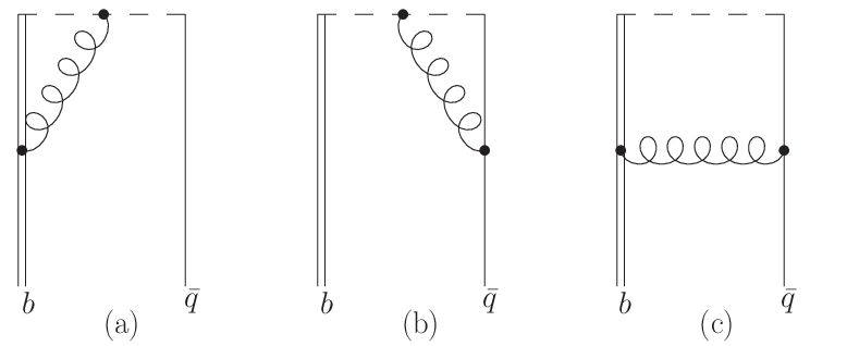
We get to by calculating the convolution integrals occurring in (C.5) in both QCD and HQET up to . The corresponding diagrams are shown in fig. C.1. As in section 3.3 we can use the wave functions (C.1), (C.2) defined by free quark states instead of hadronic states. We assign to the -quark the momentum ( resp.) in the case of pure QCD (HQET resp.) and to the soft constituent quark, where is the four velocity of the -meson. At tree level we get for both QCD and HQET the same wave function:
| (C.7) |
where the spinor fulfils the condition , and our convolution integral is
| (C.8) |
At NLO only the first diagram in fig. C.1 needs to be considered as the other two are in leading power identical for QCD and HQET. The following expressions are given in the scheme, i.e. we redefine . For the diagram in fig. C.1(a) we get in QCD
| (C.9) |
and in HQET
| (C.10) |
The wave function renormalisation constants of the heavy quark field are given in the onshell scheme for the QCD -field:
| (C.11) |
and for the HQET field :
| (C.12) |
The renormalisation of the -field drops out in the matching. Diagrammatically the matching equation (C.5) reads:
| (C.13) |
Finally we obtain
| (C.14) |
where we have renormalised the UV-divergences in the -scheme.
Bibliography
- [1] L. Wolfenstein, Phys. Rev. Lett. 51, 1945 (1983).
- [2] A. J. Buras, M. E. Lautenbacher and G. Ostermaier, Phys. Rev. D50, 3433 (1994), [hep-ph/9403384].
- [3] CKMfitter Group, J. Charles et al., Eur. Phys. J. C41, 1 (2005), [hep-ph/0406184], updates at http://ckmfitter.in2p3.fr.
- [4] BELLE, K. Abe et al., Phys. Rev. D71, 072003 (2005), [hep-ex/0408111].
- [5] BABAR, B. Aubert et al., Phys. Rev. D73, 012004 (2006), [hep-ex/0507054].
- [6] BABAR, e. Harrison, P. F. and e. Quinn, Helen R., Papers from Workshop on Physics at an Asymmetric B Factory (BaBar Collaboration Meeting), Rome, Italy, 11-14 Nov 1996, Princeton, NJ, 17-20 Mar 1997, Orsay, France, 16-19 Jun 1997 and Pasadena, CA, 22-24 Sep 1997.
- [7] Heavy Flavor Averaging Group (HFAG), E. Barberio et al., [hep-ex/0603003], updates at http://www.slac.stanford.edu/xorg/hfag.
- [8] M. Beneke, G. Buchalla, M. Neubert and C. T. Sachrajda, Phys. Rev. Lett. 83, 1914 (1999), [hep-ph/9905312].
- [9] M. Beneke, G. Buchalla, M. Neubert and C. T. Sachrajda, Nucl. Phys. B591, 313 (2000), [hep-ph/0006124].
- [10] M. Beneke, G. Buchalla, M. Neubert and C. T. Sachrajda, Nucl. Phys. B606, 245 (2001), [hep-ph/0104110].
- [11] G. Bell, [arXiv:0705.3133 [hep-ph]].
- [12] G. Bell, [arXiv:0705.3127 [hep-ph]].
- [13] M. Beneke and S. Jäger, Nucl. Phys. B751, 160 (2006), [hep-ph/0512351].
- [14] N. Kivel, [hep-ph/0608291].
- [15] C. W. Bauer, S. Fleming, D. Pirjol and I. W. Stewart, Phys. Rev. D63, 114020 (2001), [hep-ph/0011336].
- [16] C. W. Bauer, D. Pirjol and I. W. Stewart, Phys. Rev. D65, 054022 (2002), [hep-ph/0109045].
- [17] M. Beneke, A. P. Chapovsky, M. Diehl and T. Feldmann, Nucl. Phys. B643, 431 (2002), [hep-ph/0206152].
- [18] G. Buchalla, A. J. Buras and M. E. Lautenbacher, Rev. Mod. Phys. 68, 1125 (1996), [hep-ph/9512380].
- [19] M. Gronau, O. F. Hernandez, D. London and J. L. Rosner, Phys. Rev. D50, 4529 (1994), [hep-ph/9404283].
- [20] K. G. Chetyrkin and F. V. Tkachov, Nucl. Phys. B192, 159 (1981).
- [21] F. V. Tkachov, Phys. Lett. B100, 65 (1981).
- [22] S. Laporta, Int. J. Mod. Phys. A15, 5087 (2000), [hep-ph/0102033].
- [23] G. Passarino and M. J. G. Veltman, Nucl. Phys. B160, 151 (1979).
- [24] T. Gehrmann and E. Remiddi, Nucl. Phys. B580, 485 (2000), [hep-ph/9912329].
- [25] E. Remiddi, Nuovo Cim. A110, 1435 (1997), [hep-th/9711188].
- [26] M. Caffo, H. Czyz, S. Laporta and E. Remiddi, Nuovo Cim. A111, 365 (1998), [hep-th/9805118].
- [27] S. G. Gorishnii, Nucl. Phys. B319, 633 (1989).
- [28] M. Beneke and V. A. Smirnov, Nucl. Phys. B522, 321 (1998), [hep-ph/9711391].
- [29] V. A. Smirnov, Commun. Math. Phys. 134, 109 (1990).
- [30] V. A. Smirnov, Springer Tracts Mod. Phys. 177, 1 (2002).
- [31] G. Duplančić and B. Nižić, Eur. Phys. J. C20, 357 (2001), [hep-ph/0006249].
- [32] S. Herrlich and U. Nierste, Nucl. Phys. B455, 39 (1995), [hep-ph/9412375].
- [33] A. F. Falk, B. Grinstein and M. E. Luke, Nucl. Phys. B357, 185 (1991).
- [34] G. P. Lepage and S. J. Brodsky, Phys. Rev. D22, 2157 (1980).
- [35] B. O. Lange and M. Neubert, Phys. Rev. Lett. 91, 102001 (2003), [hep-ph/0303082].
- [36] M. Jamin and B. O. Lange, Phys. Rev. D65, 056005 (2002), [hep-ph/0108135].
- [37] A. Khodjamirian, T. Mannel and N. Offen, [hep-ph/0611193].
- [38] A. Abada et al., Nucl. Phys. B619, 565 (2001), [hep-lat/0011065].
- [39] E. Dalgic et al., Phys. Rev. D73, 074502 (2006), [hep-lat/0601021].
- [40] A. Khodjamirian, R. Rückl, S. Weinzierl, C. W. Winhart and O. I. Yakovlev, Phys. Rev. D62, 114002 (2000), [hep-ph/0001297].
- [41] M. Göckeler et al., Nucl. Phys. Proc. Suppl. 161, 69 (2006), [hep-lat/0510089].
- [42] V. M. Braun et al., Phys. Rev. D74, 074501 (2006), [hep-lat/0606012].
- [43] Particle Data Group, W. M. Yao et al., J. Phys. G33, 1 (2006), updates at http://pdg.lbl.gov.
- [44] A. Khodjamirian, T. Mannel and N. Offen, Phys. Lett. B620, 52 (2005), [hep-ph/0504091].
- [45] V. M. Braun, D. Y. Ivanov and G. P. Korchemsky, Phys. Rev. D69, 034014 (2004), [hep-ph/0309330].
- [46] A. G. Grozin and M. Neubert, Phys. Rev. D55, 272 (1997), [hep-ph/9607366].
- [47] S. J. Lee and M. Neubert, Phys. Rev. D72, 094028 (2005), [hep-ph/0509350].
- [48] M. Beneke and M. Neubert, Nucl. Phys. B675, 333 (2003), [hep-ph/0308039].
- [49] M. Beneke and S. Jäger, Nucl. Phys. B768, 51 (2007), [hep-ph/0610322].
- [50] M. Jamin and M. E. Lautenbacher, Comput. Phys. Commun. 74, 265 (1993).
Acknowledgements
There are many people who contributed to the present thesis. First of all I would like to thank my advisor Prof. Gerhard Buchalla. He made my PhD studies possible by supplying me with a scholarship of the “Graduiertenkolleg Particle Physics at the Energy Frontier of New Phenomena”. I also want to thank him for many inspiring discussions.
I am particularly indebted to Guido Bell for giving me useful hints and for stimulating discussions, where I learned much about technical details in the calculations of Feynman integrals. I would also like to thank my room mate Matthäus Bartsch and Sebastian Jäger for many instructive and helpful discussions.
Furthermore I want to thank Matthäus Bartsch, Guido Bell, Gerhard Buchalla and Sebastian Jäger for proofreading the drafts and comments on the manuscript.
Finally I want to thank my parents, whose aid made my physics studies possible.