Non-perturbative renormalization-group approach to zero-temperature Bose systems

In spite of the success of the Bogoliubov theory in providing a microscopic explanation of superfluidity [1], a clear understanding of the infrared behavior of interacting boson systems at zero temperature has remained a challenging theoretical issue until very recently. Besides approximations that do not satisfy the Goldstone-Hugenholtz-Pines theorem [2, 3], first attempts to improve the Bogoliubov theory revealed a singular perturbation theory plagued by infrared divergences due to the presence of the Bose-Einstein condensate and the Goldstone mode [4, 5]. These divergences cancel in most physical quantities but lead to a vanishing of the anomalous self-energy $\Sigma_{\rm an}(q)$ in the limit $q\equiv({\bf q},\omega)\to 0$ although the linear spectrum and therefore the superfluidity are preserved [6, 7, 8, 9]. This observation seriously called into question the validity of the Bogoliubov theory, where the linear spectrum relies on a finite value of $\Sigma_{\rm an}(q\to 0)$ [10]. The physical origin of the vanishing of the anomalous self-energy is the divergence of the longitudinal correlation function which is driven by the gapless (transverse) Goldstone mode – a general phenomenon in systems with a continuous broken symmetry [11].

The infrared behavior of zero-temperature Bose systems is now well understood in the modern language of renormalization group (RG) [12, 13, 14, 15]. Using a field-theoretical renormalization-group approach supplemented by the Ward identities associated with the gauge symmetry, Castellani et al. were able to establish the exact infrared behavior of a zero-temperature Bose system [14, 15]. Only for $d>3$ does the Bogoliubov theory predict the correct infrared behavior, whereas the Bogoliubov fixed point is found to be unstable for $d\leq 3$ even though the low-energy mode remains phonon-like with a linear spectrum. In the approach of Refs. [14, 15], the low-energy behavior of the correlation functions is expressed exactly in terms of thermodynamics quantities such as the density, the condensate density or the macroscopic sound velocity. Despite its very elegant formulation, this approach however does not appear to enable an explicit calculation of the correlation functions in terms of the parameters of a particular microscopic model. Given the present possibilities to realize low-dimensional and/or strongly correlated Bose systems in ultracold atomic gases [16], it would be of great interest to have a theoretical framework allowing for quantitative predictions that could be tested against the experimental results.

In this Letter, we use a non-perturbative renormalization-group (NPRG) technique [17, 18, 19, 20] to study interacting bosons at zero temperature. Not only does our approach give the exact asymptotic behavior of the correlation functions in dimensions $d>1$ within a rather simple theoretical framework free of infrared divergences, but it also enables to explicitely follow the behavior of the system from microscopic to macroscopic scales. In one-dimension and for not too strong interactions, it yields a good picture of the Luttinger-liquid behavior of the superfluid phase. NPRG studies of interacting bosons have previously been reported both at finite [21] and zero [22] temperature. To a large extent, our results are complementary to those of Ref. [22].

We consider the following action,

where $\psi(x)$ is a bosonic (complex) field, $x=({\bf r},\tau)$, $\int dx=\int_{0}^{\beta}d\tau\int d^{d}r$. $\tau\in[0,\beta]$ is an imaginary time, $\beta\to\infty$ the inverse temperature, and $\mu$ denotes the chemical potential. The interaction is assumed to be local in space and the model is regularized by a momentum cutoff $|{\bf q}|<\Lambda$ (with $\Lambda\to\infty$ whenever convenient). We take $\hbar=k_{B}=1$ throughout the Letter.

The basic quantity of interest in the NPRG is the effective action $\Gamma[\phi]$, which is the generating functional of the one-particle irreducible (1PI) vertices. It is obtained by a Legendre transform of the free energy $\ln Z[J]$ computed in the presence of an external source term $S_{J}=\int dx[J^{*}(x)\psi(x)+{\rm c.c.}]$ ($\phi=\langle\psi\rangle_{J}$) [19, 22]. To implement the RG procedure, we add to the action an infrared regulator $\Delta S_{R}=\int dx\,\psi^{*}(x)R(x-x^{\prime})\psi(x^{\prime})$ which suppresses the fluctuations with ${\bf q}^{2}<k^{2}$. The functional $\Gamma[\phi]\equiv\Gamma_{k}[\phi]$ then becomes $k$ dependent and satisfies the exact flow equation

where we have introduced the flow parameter $t=\ln(k/\Lambda)$. In Fourier space, the trace in (2) involves a sum over frequencies and momenta, as well as a trace over the two indices of the complex field $\phi$. $\Gamma^{(2)}[\phi]$ is the second-order functional derivative of $\Gamma[\phi]$ with respect to $\phi$. Choosing $R$ to diverge for $k\to\infty$, all fluctuations are then suppressed and the mean-field theory, where the effective action $\Gamma[\phi]$ reduces to the microscopic action $S[\phi]$, becomes exact. Quantum fluctuations are gradually taken into account by decreasing $k$ and making use of (2). For $k=0$, $\Gamma[\phi]$ corresponds to the effective action of the original model (1) from which we can deduce all 1PI vertices – and in particular the single-particle propagator $G=-\Gamma^{(2)-1}$ – as well as the thermodynamic potential.

The functional differential equation (2) is too complicated to be solved exactly. For approximate solutions it is sufficient to truncate the most general form of $\Gamma[\phi]$ [19, 22]. For a superfluid Bose system, the simplest choice reads

where $n(x)=|\phi(x)|^{2}$ is the density. Eq. (3) is obtained from an expansion to fourth order about the minimum $|\phi(x)|=\sqrt{n_{0}}$, where $n_{0}$ denotes the condensate density. We use a derivative expansion to order ${\cal O}(\partial^{2})$ [19, 23]. For $k\to\infty$, the initial conditions are $Z=Z_{1}=1$, $V=0$, $\lambda=g$ and $n_{0}=\mu/g$, and the effective action $\Gamma[\phi]$ reproduces the Bogoliubov theory. Although $V$ is not present in the original action (1), it is always generated by the flow equation (2) [22] and plays a crucial role when $d\leq 3$. The degeneracy of the minimum $|\phi(x)|=\sqrt{n_{0}}$ reflects the gauge invariance (i.e. the U(1) symmetry $\psi^{(*)}(x)\to\psi^{(*)}(x)e^{\pm i\alpha}$) of the action (1). A broken-symmetry state can be obtained by picking up a particular minimum. It is convenient to write $\phi=(\phi_{1}+i\phi_{2})/\sqrt{2}$ in terms of two real fields $\phi_{1}$ and $\phi_{2}$ and to consider the state $\bar{\phi}=(\sqrt{2n_{0}},0)$ as an example of broken-symmetry state. In Fourier space, the corresponding single-particle vertex $\bar{\Gamma}^{(2)}=-\bar{G}^{-1}$ (with $\bar{G}_{ij}=-\langle\psi_{i}\psi_{j}\rangle$) then reads

($\epsilon_{\bf q}={\bf q}^{2}/(2m)$). The vanishing of $\bar{\Gamma}_{22}(q=0)$, which is a mere consequence of the U(1) symmetry, naturally implements the Hugenholtz-Pines theorem [3, 24] in our formalism. The combination $\lambda n_{0}$ corresponds to the anomalous self-energy $\Sigma_{\rm an}(q=0)$. There are two important quantities that can be read off from (4), namely the superfluid density $n_{s}$ and the Goldstone mode velocity $c$,

For $k\to\infty$, one has $n_{s}=n_{0}=\mu/g$ and $c=\sqrt{n_{0}g/m}$. The superfluid density is defined in the usual way from the stiffness of the system with respect to a twist of the phase of the superfluid order parameter $\bar{\phi}=(\sqrt{2n_{0}},0)$. The expression of the velocity $c$ follows from the equation ${\rm det}\,\bar{\Gamma}^{(2)}(q)=0$ in the limit $q\to 0$.

Inserting (3) into (2), we obtain the flow equations

where $A=1+Z_{2}\omega^{2}$, $B=A+2M$, $D=AB+\omega^{2}$, $M=\tilde{\lambda}\tilde{n}_{0}$, $v_{d}^{-1}=2^{d+1}\pi^{d/2}\Gamma(d/2)$, $s=(v_{d}/d)[1-\eta/(d+2)]$, and $\int_{\omega}=\int d\omega/(2\pi)$. We have introduced the dimensionless quantities

as well as $\eta=-\partial_{t}\ln Z$ and $\eta_{1}=-\partial_{t}\ln Z_{1}$, and chosen the regulator $R({\bf q}^{2})=Z(\epsilon_{k}-\epsilon_{\bf q})\theta(\epsilon_{k}-\epsilon_{\bf q})$ [25]. $\Omega$ denotes the thermodynamic potential per unit volume in the broken-symmetry state $\bar{\phi}=(\sqrt{2n_{0}},0)$. For $Z_{2}=0$ (i.e. $V=0$), the integrals over $\omega$ can be carried out and we reproduce the flow equations derived in Ref. [22]. However, the approximation $V=0$ – or a mere perturbative treatment of $V$ – cannot be used for $d\leq 3$ as it predicts the wrong exponent ($2\epsilon$ instead of $\epsilon=3-d$) for the divergence of the longitudinal correlation function, the wrong lower critical dimension (2 instead of 1), and – for $V=0$ – an infinite velocity for the Goldstone mode.

When $d>1$, superfluidity is always accompanied by Bose-Einstein condensation (BEC): $\lim_{k\to 0}n_{0}=n_{0}^{*}>0$. For $d>3$, the Bogoliubov fixed point is stable; all parameters in the effective action $\Gamma_{t=0}$ remain finite as $k\to 0$. $V^{*}=\lim_{k\to 0}V$, although nonzero, gives only a finite correction to the infrared limit of the vertices. This picture changes dramatically when $d\leq 3$. In this case, both $Z_{1}$ and $\lambda$ are suppressed as $k\to 0$, which explains why the anomalous self-energy $\Sigma_{\rm an}(q=0)=\lambda n_{0}$ vanishes in the infrared limit. This suppression is logarithmic for $d=3$ and powerlaw-like in lower dimensions. When $d>1$, we can use the fact that $\lim_{k\to 0}M=\lim_{k\to 0}Z_{2}M=\infty$ to analytically obtain the asymptotic behavior for $k\to 0$ (table 1). A typical RG flow in two dimensions is shown in Figs. 1 and 2.

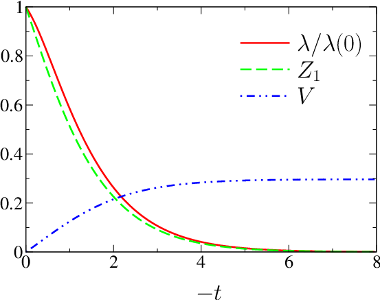
The suppression of $Z_{1}$, together with a finite $V^{*}$, shows that the effective action exhibits a space-time SO($d$+1) symmetry in the infrared limit [22]. This limit is well understood and corresponds to the classical O(2) model in $d+1$ dimensions. The symmetry can be made explicit by the rescaling $\tilde{\bf r}=k{\bf r}$, $\tilde{\tau}=(Z_{1}\epsilon_{k}^{-1}\sqrt{Z_{2}})^{-1}\tau$ and $\tilde{\phi}(\tilde{x})=(ZZ_{1}\sqrt{Z_{2}}k^{-d})^{1/2}\phi(x)$, whereby the effective action becomes

where $\tilde{n}_{0}^{\prime}=\sqrt{Z_{2}}\tilde{n}_{0}$ and $\tilde{\lambda}^{\prime}=\tilde{\lambda}/\sqrt{Z_{2}}$. For a typical frequency $\tilde{\omega}\sim k$, the term linear in $\partial_{\tilde{\tau}}$ becomes subleading with respect to the quadratic one. Equivalently, one can observe that for $d\leq 3$ the Goldstone mode velocity reaches the fixed point value $c^{*}=(Z^{*}/2mV^{*})^{1/2}$ which is independent of $Z_{1}$. Our numerical results for the scaling of $\tilde{n}_{0}^{\prime}$ and $\tilde{\lambda}^{\prime}$ agree with the known results for the Goldstone regime of the classical O(2) model in $d+1$ dimensions (table 1). The dimensionless coupling $\tilde{\lambda}^{\prime}$ vanishes for $d=3$ and flows to a finite value for $d<3$. The relation $2\eta_{1}^{*}+\eta_{2}^{*}=-2$ (with $\eta_{2}=-\partial_{t}\ln Z_{2}$) ensures that the Goldstone mode velocity reaches a finite value for $k\to 0$, i.e. that the dynamical exponent takes the value $z=1$.

There are three important relations between 1PI vertices and thermodynamic quantities that our results should fulfill,

The equality of the superfluid density $n_{s}$ and the density $n$ is a consequence of Galilean invariance at zero temperature. Since the chemical potential appears only in the initial conditions for the effective action $\Gamma[\phi]$, derivatives with respect to $\mu$ can be numerically calculated by solving the flow equations for nearby values of $\mu$. The equality between the Goldstone mode velocity $c$ and the macroscopic sound velocity $c_{s}$ was proved in Ref. [5]. The last relation in (10) is a consequence of gauge invariance [15]. The figures 3, 4 and 5 show that the symmetry constraints (10), despite a good overall agreement, are not strictly enforced in our approach. This can be ascribed to the choice of our infrared regulator $R({\bf q}^{2})$ as well as the Ansatz (3) which are both incompatible with Galilean invariance.

Making use of (10), we can rewrite the propagator $\bar{G}(q)=-\bar{\Gamma}^{(2)-1}(q)$ as

in the infrared limit. In (11), all quantities except $\lambda$ can be evaluated at $k=0$. Because of the vanishing of $\lambda(k\to 0)$, the longitudinal correlation function $\bar{G}_{11}$ diverges logarithmically in three dimensions and as $k^{-\epsilon}$ below [6, 7, 9]. (see table 1). The dependence on $q$ can be restored by evaluating $\lambda$ at $k\sim\sqrt{\omega^{2}+c^{2}{\bf q}^{2}}$. In Ref. [15], the equations (11) were obtained by imposing the Ward identities due to gauge invariance and solving a one-loop RG equation for the sole independent coupling in the limit $k\to 0$ [26]. By a detailed analysis of the structure of the perturbation theory to higher order, it was then argued that the equations (11) give the exact asymptotic behavior. We believe that our RG approach, being intrinsically non-perturbative [19], gives further support to this claim.

In one-dimension, as a result of the emerging SO(2) symmetry, we find that the long-distance physics is described by the classical O(2) model in $d+1=2$ dimensions [22]. We thus expect the system to be in the “low-temperature” phase of the Kosterlitz-Thouless phase transition. There is no BEC as the condensate density $n_{0}\sim k^{\eta^{*}}$ vanishes in the thermodynamic limit $k\to 0$. However, the superfluid density $n_{s}=Zn_{0}$ remains finite. This phase is generally described as a Luttinger liquid (LL) characterized by the Goldstone mode velocity $c^{*}$ and the LL parameter $K$ [27, 28].

It has been shown that the NPRG gives a good description of the classical O(2) model [29, 30]. In particular the low-temperature phase is characterized by an approximate line of fixed points where the beta function becomes very small and the running of the renormalized order parameter $\tilde{n}_{0}^{\prime}$ (or, equivalently, the phase stiffness) very slow, which implies a very large, although not strictly infinite, correlation length $\xi$. The anomalous exponent $\eta$ depends on the (slowly running) order parameter $\tilde{n}_{0}^{\prime}$ and takes its largest value $\sim 1/4$ when the system crosses over to the disordered regime ($k\sim\xi^{-1}$).

By solving numerically the flow equations (7) in one dimension, we have obtained very similar results. Figs. 6 and 7 show the flow trajectories in the space $(n_{s},c,\tilde{\lambda}^{\prime})$ for various initial conditions $n_{0}(t=0)$ and $\lambda(t=0)$. The points correspond to equal steps in $t$ so that very dense points indicate a very slow running. For a sufficiently small ratio $\lambda(t=0)/n_{0}(t=0)$, we find that trajectories rapidly hit an approximate plane of fixed points defined by $\tilde{\lambda}^{\prime}\sim 15$, where the running of the superfluid density $n_{s}$ and the Goldstone mode velocity $c$ become very slow. As for the classical O(2) model, we infer from this observation that the correlation length $\xi$ is extremely large for these trajectories. For very long RG time $-t$ ($k\sim\xi^{-1}$), the system eventually crosses over to the disordered regime. On the approximate plane of fixed points, the scale-dependent anomalous exponent $\eta$ varies slowly about a value that depends both on $n_{s}$ and $c$ (Fig. 8). It then reaches its maximum value $\eta_{c}\simeq 0.29$ – to be compared with the exact exponent $\eta_{c}=1/4$ at the Kosterlitz-Thouless transition of the classical O(2) model – before rapidly dropping to zero once $k\sim\xi^{-1}$. For $M\gg 1$, which corresponds to a large superfluid density $n_{s}$, we obtain the analytic expression $\eta=mc/(2\pi n_{s})$ from (7). This in turn determines the LL parameter $K=1/(2\eta)=\pi n_{s}/(mc)$, which is the expected value in a Galilean invariant system where $n_{s}=n$ [27].

Thus for a sufficiently small ratio $\lambda(t=0)/n_{s}$ (or $c/n_{s}$), we obtain a good picture of the Luttinger liquid behavior of the superfluid phase. When this ratio is too large, the flow trajectory does not reach the approximate plane of fixed points, and the system is in the “high-temperature” (disordered) phase of the classical O(2) model. This result is in contradiction with known results in one dimension where the action (1) corresponds to the exactly soluble Lieb-Liniger model [31, 32]. This model is parameterized by the dimensionless parameter $\gamma=m\lambda(t=0)/n$ and its low-energy description is a Luttinger liquid with a parameter $K\equiv K(\gamma)$ varying in the interval $[1,\infty[$ as $\gamma$ decreases from infinity to zero [28]. The limit $\gamma\to\infty$ ($K=1$) corresponds to hard-core bosons. Thus the anomalous exponent $\eta$ should take its highest value $1/(2K_{\rm min})=1/2$ for $\gamma\to\infty$ rather than $1/4$ as predicted by our results. A possible explanation for the failure of our approach to correctly describe the strong-coupling limit of the action (1) in one dimension is the derivative expansion used in the Ansatz (3) for $\Gamma[\phi]$. Quite generally, the derivative expansion is known to work best when $\eta$ is small [19, 20].

The NPRG technique discussed in this Letter provides an efficient method to control the infrared divergences appearing in the perturbation theory of zero-temperature Bose systems. It extends the approach of Ref. [22] and reproduce the results obtained earlier by a field-theoretical RG approach combined with the implementation of Ward identities due to gauge invariance [14, 15]. The non-trivial infrared behavior in dimensions $1<d\leq 3$, characterized by the divergence of the longitudinal correlation function and the vanishing of the anomalous self-energy $\Sigma_{\rm an}(q\to 0)$, turns out to be related to the emergence of a space-time SO($d$+1) symmetry at low energy. This implies a close link between the superfluid phase and the Goldstone regime of the classical O(2) model in $d+1$ dimension [22].

Our approach also describes one-dimensional systems where superfluidity exists without BEC in the thermodynamic limit. The superfluid phase exhibits a Luttinger-liquid behavior that is well captured by the NPRG approach for weak interactions. Although our results, based on a derivative expansion of the effective action $\Gamma[\phi]$, break down at strong coupling, they might be improved by a more refined treatment of the momentum dependence of the vertices [33].

An important feature of the NPRG is that it not only yields the infrared behavior of correlation functions but can also compute propagators in terms of the parameters of a microscopic model. It thus provides an efficient tool for the explicit calculation of physical quantities beyond the Bogoliubov theory while satisfying basic requirements such as the Hugenholtz-Pines theorem as well as yielding the correct infrared behavior, a task that has been known to be difficult in interacting boson systems [2, 34].