Transport properties controlled by a thermostat: An extended dissipative particle dynamics thermostat
Abstract
We introduce a variation of the dissipative particle dynamics (DPD) thermostat that allows for controlling transport properties of molecular fluids. The standard DPD thermostat acts only on a relative velocity along the interatomic axis. Our extension includes the damping of the perpendicular components of the relative velocity, yet keeping the advantages of conserving Galilei invariance and within our error bar also hydrodynamics. This leads to a second friction parameter for tuning the transport properties of the system. Numerical simulations of a simple Lennard-Jones fluid and liquid water demonstrate a very sensitive behaviour of the transport properties, e.g., viscosity, on the strength of the new friction parameter. We envisage that the new thermostat will be very useful for the coarse-grained and adaptive resolution simulations of soft matter, where the diffusion constants and viscosity of the coarse-grained models are typically too high/low, respectively, compared to all-atom simulations.
pacs
02.70.Ns, 05.10.-a, 61.20.Ja, 61.25.EmI Introduction
Using the optimal set of degrees of freedom (DOFs) in computer simulations of soft matter guarantees efficiency, accuracy and avoids huge amounts of unnecessary detail, which might even obscure the underlying physics. This very idea is exploited in systematic coarse-graining efforts for modern computational materials science and biophysics problems Harmandaris:2006; Hess:2006; Nico:2007, where atomistic simulations are usually beyond the possibilities of current and near future computers. A similar philosophy of reducing the number of DOFs is also employed by representing clusters of molecules with soft particles when simulating fluids on a mesoscopic scale using dissipative particle dynamics (DPD)Hoogerbrugge:1992; Koelman:1993; Espanol:1995; Groot:1997; Espanol:1998. However, in typical soft matter systems different time- and length-scales are intrinsically interconnected and a multiscale modeling approach is required to tackle such problems in the most efficient wayDelleSite:2002; Delgado:2003; Barsky:2004; Delgado:2005; Neri:2005; Villa:2005; Fabritiis:2006; Voth2006.
Recently, we have proposed an adaptive resolution scheme (AdResS) that couples the atomistic and coarse-grained levels of detailPraprotnik:2005:4; Praprotnik:2006; Praprotnik:2007; Praprotnik:2007:1; Praprotnik:2007:3; Praprotnik:2007:2. Due to the reduction in DOFs upon coarse-graining, which eliminates the fluctuating forces associated with those missing molecular DOFs, the coarse-grained molecules typically move faster than the corresponding atomistically resolved onesTschop:1998; Izvekov:2006. Although the accelerated dynamics is advantageous in some cases it can turn out to be problematic if one is really interested in dynamics in situations where two levels of resolutions are used within one simulation, as in the case of AdResS. To overcome this problem one can couple different classes of DOFs to the Langevin thermostat with different friction constantscarmeli; moix; grigolini; voth. We have shown in the example of liquid water that the coarse-grained dynamics can be slowed down by increasing the effective friction in the coarse-grained systemwater2. However, it is well known that the Langevin thermostat does not reproduce the correct hydrodynamics, i.e., the hydrodynamic interactions are unphysically screened. In order to correctly describe hydrodynamic interactions, one has to resort to the DPD thermostatSoddemann:2003.
In the past years DPD has established itself as a useful thermostat for soft matter simulations. The DPD thermostat is known to have several good properties, i.e., the thermostat satisfies Newton’s third law by construction and owing to mass, momentum and temperature conservation, hydrodynamics is also correctly reproduced Espanol:1995:2. As it turns out, however, the DPD thermostat in its standard form is not capable of controlling liquid properties such as viscosity and diffusion constantSoddemann:2003. The aim of this work is to extend the DPD equations in such a way that these quantities can be tuned by changing the parameters of the thermostat. We consider the most general version of DPDEspanol:1995 and exploit the terms, which are not used in the standard DPD approach, i.e., the damping of the perpendicular components of the relative particle velocities. This allows us to tune the viscosity of the coarse-grained liquid to match that of the all-atom counterpart while conserving the virtues of the standard DPD thermostat. This should be very useful for both coarse-grained and adaptive resolution simulations of soft matter.
The article is organized as follows: In Sec. II the standard and new DPD thermostats are presented. The simulation setup is described in Sec. III. The results of molecular dynamics (MD) simulations of the Lennard-Jones fluid and liquid water are reported in Sec. IV, followed by the conclusions in Sec. V.
II Thermostats
II.1 Standard DPD thermostat
Newton’s equations of motion are used in microcanonical NVE MD simulations and generate dynamics with constant energy. In order to run simulations in the canonical NVT ensemble the equations of motion have to be modified. In Langevin dynamics two additional forces are introduced, a damping and a random force, whose ratio defines the temperature. The DPD equations of motion (used by the DPD thermostat) are then given byHoogerbrugge:1992; Espanol:1995
| (1) |
and
| (2) |
where denotes the conservative force on the th particle. The damping and random forces, can be split up in particle pair forces as
| (3) |
| (4) |
where the dissipative force reads asEspanol:1995
| (5) |
and the random force is given by
| (6) |
In these equations the relative velocity between the th and th particle was introduced, while denotes the unit vector of the interatomic axis . is the friction constant and the noise strength. and are -dependent weight functions. These are connected by the fluctuation-dissipation theorem (see Eqn. (9)). The variable is symmetric in the particle indices () and has the following first
| (7) |
and second moment
| (8) |
The fluctuation-dissipation theorem Espanol:1995 reads as
| (9) |
and
| (10) |
The above DPD equations conserve the total momentum and reproduce correctly the hydrodynamics interactions in the system. However, previous studies Soddemann:2003; Marsh:1997 have shown that the strength of the friction does not influence the viscosity in linear order. In order to be able to tune the value of the viscosity of the system while preserving all of the virtues of the standard DPD thermostat presented briefly above we introduce in the next subsection its extension named “Transverse DPD thermostat”.
II.2 Transverse DPD thermostat
We generalize Eqn. (5) and Eqn. (6) as
| (11) |
and
| (12) |
where and are the friction constant and the noise strength of the generalized thermostat, respectively (see the text below). is a projection operator
| (13) |
which is symmetric in the particle indices (). The scalar noise (see Eqn. (8)) is replaced by a noise vector
| (14) |
which is antisymmetric in the particle indices () due to the symmetry of the projection operator and the antisymmetry of the pair force (Newton’s third law). The corresponding Fokker-Planck operator is a sum of two parts: the deterministic part
| (15) |
and the generalized DPD part
The equilibrium condition then yields the dissipation-fluctuation-theorem in the same form as given by Eqn. (9) and Eqn. (10).
For the case where we choose the projector along the interatomic axis between particle and
| (17) |
we retain the standard DPD thermostat.
Alternatively, one can project on the plane perpendicular to the interatomic axis
| (18) |
The space defined by the projector (18) is orthogonal to the case of the standard DPD and introduces an extension of the DPD thermostat, i.e., the Transverse DPD thermostat. Note that owing to this orthogonality the new thermostat can be used in combination with the standard one. This enables us to adjust at the same time two friction constants and for the standard and Transverse DPD thermostats, respectively. Galilei invariance remains valid by construction while hydrodynamics is conserved within our error barangular_momentum.
Our basic assumption is that in contrast to the standard DPD the viscosity is very sensitive to the damping perpendicular to the interatomic axis. This damping mimics the shear of those DOFs that were integrated out in the coarse-graining procedure. In a system with two particles the stochastic forces of the Transverse DPD thermostat act in the same direction as the shear forces. The mean force acting on a particle in the sheared system with more than two particles is hence a sum of two contributions: a force coming from the Transverse DPD thermostat and another one originating from the shearing of the probe. Therefore, the shear viscosity in a simulation with the Transverse DPD thermostat is always higher than with the standard one. In the Green-Kubo picture this additional viscosity arises from the projected velocity-velocity autocorrelation function, which is derived by the Mori-Zwanzig formalism Zwanzig:1960; Zwanzig:1961; Forster:1975. The exact derivation is beyond the scope of this paper and will be presented elsewhere. Here, we shall demonstrate this by the results of our numerical experiments presented in the results section.
III Simulation setup
All simulations of the Lennard-Jones (LJ) liquid and liquid water are performed using the ESPResSo package Espresso:2005.
III.1 Lennard-Jones Fluid
We use the repulsive Weeks-Chandler-Andersen (WCA) potential
| (19) |
with the cutoff at , and being the standard LJ parameters of length and energy.
We chose as the weight function (see Eqn. (10)) for both thermostats a step function
| (20) |
The simulations are carried out with a system consisting of 1000, 2000 and 4000 LJ particles at a temperature and density in a cubic box with periodic boundary conditions.
III.2 Liquid Water
All-atom water NVT simulations at ambient conditions are performed using the rigid TIP3P water modelJorgensen:1983. The electrostatics is described by the reaction field (RF) method, in which all molecules outside a spherical cavity of a molecular based cutoff radius Å are treated as a dielectric continuum with a dielectric constant Neumann:1983; Neumann:1985; Tironi:1995. Typically, all-atom water simulations are carried out using global thermostats, e.g., BerendsenBerendsen:1984, Nosé-HooverNose:1984; Hoover:1985, Nosé-Hoover chainsMartyna:1992 thermostats, that dissipate the energy uniformly in the system. Local thermostats, e.g., Langevin, DPDSoddemann:2003, AndersenAndersen:1980, Lowe-AndersenLowe:1999; Peters:2004; Koopman:2006, Nosé-Hoover-Lowe-AndersenStoyanov:2005 thermostats, that dissipate energy on a spatially localized scale are usually used in coarse-grained simulations. Here, in order to reproduce the hydrodynamics correctly we employed the DPD thermostatSoddemann:2003 with the friction constant and cutoff radius . The constant is small compared to the intrinsic friction coefficient of the TIP3P water system, i.e., , so that the stochastic dynamics yields the correct dynamicsKremer:1990; water2. For the coarse-grained water simulations with the Transverse DPD thermostat we have employed the single-site water model from Ref.Praprotnik:2007:2, which reproduces essential thermodynamics and structural properties, e.g., the pressure, density, and radial distribution functions, of the all-atom rigid TIP3P water model at standard conditions. Other simulation details are the same as given in Ref.Praprotnik:2007:2.
IV Results
IV.1 Lennard-Jones Fluid
First, we checked in an equilibrium simulation the dependency of pressure and temperature on the strength of the friction. We set the reference temperature to and measured the instantaneous temperature defined as
| (21) |
where and are the kinetic energy and the number of particles of the system, respectively. The relative deviation between the measured and reference temperature was smaller then for all strengths of friction and all combination of thermostats. The mean pressure at that temperature turned out to be , which is in a perfect agreement with the results of previous studies Dunweg:1993.
Next, we studied the dependency of the liquid transport properties, i.e., the diffusion constant and shear viscosity, on the friction constants and for the standard and Transverse DPD thermostats, respectively.
IV.1.1 Diffusion constant
The diffusion constant was computed from the particle displacements using the Einstein relation
| (22) |
A small influence on this constant from the standard DPD thermostat Soddemann:2003 is expected, but a considerable one from the new Transverse DPD thermostat. Former results Soddemann:2003 for the standard DPD thermostat could be confirmed. The value of the diffusion constant approaches the equilibrium value () for vanishing friction of the Transverse DPD thermostat (see Fig. 1).
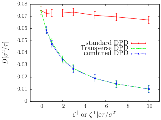
The diffusion constant is very sensitive on the friction for the Transverse DPD thermostat. By changing it is therefore possible to tune the diffusion constant.
IV.1.2 Shear viscosity
The viscosity was measured in nonequilibrium molecular dynamics (NEMD) simulation by shearing the system with a constant shear rate in the -directionSoddemann:2003
| (23) |
The viscosity can then be determined by the following simple formula
| (24) |
where is the mean force (momentum transfer per time unit). The apparent shear viscosity measured in NEMD simulation approaches the equilibrium viscosity with decreasing shear rate.
We found nearly no dependency on the strength of the friction for the standard DPD thermostat, (see also Ref. Soddemann:2003). In contrast the friction for the Transverse DPD thermostat gives a very sensitive means of controlling the viscosity (see Fig. 2). In the case of the combination of both thermostats the shear viscosity is mostly controlled by the Transverse DPD thermostat. In the limit of a vanishing shear rate a value of was extrapolated, which matches former results Dunweg:1993. This extrapolation has to be done due to short characteristic timescale of the LJ system. Additionally, we also checked that the equilibrium correlation of the pressure tensor is in accordance with the Green-Kubo picture: all (non-auto) off-diagonal - (off-)diagonal elements are uncorrelated, (60 of 81 possible elements are zero).

For higher values of the apparent viscosity becomes increasingly dependent on the shear rate. This is due to the fact that the dynamics is controlled in this regime by the thermostat forces (that are linear in ) and hence we end up measuring the “viscosity of the thermostat”.
IV.2 Tuning the Dynamics of Water
Having shown that the new thermostat enables us to tune the diffusion constant and viscosity of a simple liquid we apply it to an important physical example, i.e., liquid water at ambient conditions.
We first check that the structural properties do not depend on the thermostat and also that we obtain consistency between the coarse-grained and atomistic simulations. The center-of-mass radial distribution functions of the all-atom and coarse-grained system using different values of match within the line thickness (see Fig. 3).

There is an intrinsic timescale difference in the diffusive dynamics of the coarse-grained water system because of the reduced number of DOFs, i.e., the self-diffusion constant for the coarse-grained water model is approximately times larger then the corresponding all-atom one using the Langevin thermostat with the same background friction in both casesPraprotnik:2007:2. We used for the Transverse DPD thermostat () to match the diffusion constant of the coarse-grained water model to the corresponding value obtained from the all-atom simulation with the standard DPD thermostat. With a friction strength of , which is as desired very close to the above value for matching the diffusion constants, we were also able to match the viscosity to the desired value for the TIP3P water model (from our atomistic simulation with ). In this case the characteristic times for the atomistic model are much longer than the time scale of the shearing (). Therefore even with a shear rate of we are in the no shear limit and hence no extrapolation is required. The obtained diffusion constants and viscosities are in good agreement with the published dataWu:2006.
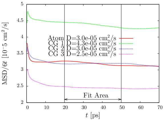
Thus, employing the new thermostat one can reproduce both the structure and the dynamics of the all-atom liquid water with the single-site coarse-grained water model. This is essential for synchronizing the timescales of the all-atom and coarse-grained regimes in the adaptive resolution MD simulationsPraprotnik:2007:2.
V Conclusions
In this paper we introduced an extension of the DPD thermostat that allows for controlling the transport properties of molecular liquids, e.g., water, while preserving the hydrodynamics.
The presented Galilean invariant local thermostat can be used in coarse-grained simulations to tune the diffusion constant and viscosity of the system to the desired values. This opens up the possibility of reproducing the atomistic dynamics by coarse-grained simulations, as it is required, for example, in recently introduced adaptive resolution simulations.
Acknowledgements
We are grateful to R. Delgado-Buscalioni and B. Dünweg for discussions at early stage of this work. We also thank J. Kirkpatrick for critical reading of the manuscript.
References
- (1) V. A. Harmandaris, N. P. Adhikari, N. F. A. Van der Vegt and K. Kremer, Macromolecules, 2006, 39, 6708–6719.
- (2) B. Hess, S. Leon, N. Van der Vegt and K. Kremer, Soft Matter, 2006, 2, 409–414.
- (3) N. F. A. van der Vegt, C. Peter and K. Kremer, Taylor and Francis, 2007.
- (4) P. J. Hoogerbrugge and J. M. V. A. Koelman, Europhys. Lett., 1992, 19, 155–160.
- (5) J. M. V. A. Koelman and P. J. Hoogerbrugge, Europhys. Lett., 1993, 21, 363–368.
- (6) P. Espaol and P. Warren, Europhys. Lett., 1995, 30, 191–196.
- (7) R. D. Groot and P. B. Warren, J. Chem. Phys., 1997, 107, 4423–4435.
- (8) P. Espaol, Phys. Rev. E, 1998, 57, 2930–2948.
- (9) L. Delle Site, C. F. Abrams, A. Alavi and K. Kremer, Phys. Rev. Lett., 2002, 89, 156103.
- (10) R. Delgado-Buscalioni and P. V. Coveney, Phys. Rev. E, 2003, 67, 046704.
- (11) S. Barsky, R. Delgado-Buscalioni and P. V. Coveney, J. Chem. Phys., 2004, 121, 2403–2411.
- (12) R. Delgado-Buscalioni, E. G. Flekkoy and P. V. Coveney, Europhys. Lett., 2005, 69, 959–965.
- (13) M. Neri, C. Anselmi, M. Cascella, A. Maritan and P. Carloni, Phys. Rev. Lett., 2005, 95, 218102.
- (14) E. Villa, A. Balaeff and K. Schulten, Proc. Natl. Acad. Sci. U.S.A., 2005, 102, 6783–6788.
- (15) G. D. Fabritiis, R. Delgado-Buscalioni and P. V. Coveney, Phys. Rev. Lett., 2006, 97, 134501.
- (16) Q. Shi, S. Izvekov and G. A. Voth, J. Phys. Chem. B, 2006, 110, 15045–15048.
- (17) M. Praprotnik, L. Delle Site and K. Kremer, J. Chem. Phys., 2005, 123, 224106.
- (18) M. Praprotnik, L. Delle Site and K. Kremer, Phys. Rev. E, 2006, 73, 066701.
- (19) M. Praprotnik, K. Kremer and L. Delle Site, Phys. Rev. E, 2007, 75, 017701.
- (20) M. Praprotnik, K. Kremer and L. Delle Site, J. Phys. A: Math. Theor., 2007, 40, F281–F288.
- (21) M. Praprotnik, L. Delle Site and K. Kremer, J. Chem. Phys., 2007, 126, 134902.
- (22) M. Praprotnik, S. Matysiak, L. Delle Site, K. Kremer and C. Clementi, J. Phys.: Condens. Matter, 2007, 19, 292201.
- (23) W. Tschöp, K. Kremer, J. Batoulis, T. Bürger and O. Hahn, Acta Polym., 1998, 49, 61–74.
- (24) S. Izvekov and G. A. Voth, J. Chem. Phys., 2006, 125, 151101.
- (25) B. Carmeli and A. Nitzan, Chem. Phys. Lett., 1983, 102, 517–522.
- (26) M. J. Moix and R. Hernandez, J. Chem. Phys., 2005, 122, 114111.
- (27) P. Grigolini, J. Chem. Phys., 1988, 89, 4300–4308.
- (28) J. B. Straus and G. A. Voth, J. Chem. Phys., 1992, 96, 5460–5470.
- (29) S. Matysiak, C. Clementi, M. Praprotnik, K. Kremer and L. Delle Site, submitted.
- (30) T. Soddemann, B. Dünweg and K. Kremer, Phys. Rev. E, 2003, 68, 046702.
- (31) P. Espaol, Phys. Rev. E, 1995, 52, 1734–1742.
- (32) C. A. Marsh, G. Backx and M. H. Ernst, Europhys. Lett., 1997, 38, 411–415.
- (33) Note that due to the Transverse DPD thermostat forces between molecules are not central and therefore the local angular momentum is not conserved. Nevertheless, simulation results show that these angular momentum fluctuations cancel out on average and hence the total angular momentum of the system is almost a conserved quantity.
- (34) R. Zwanzig, J. Chem. Phys., 1960, 33, 1338–1341.
- (35) R. Zwanzig, Phys. Rev., 1961, 124, 983–992.
- (36) D. Forster, Hydrodynamic Fluctuation, Broken Symmetry, and Correlation Functions, Benjamin, Reading, MA, 1975.
- (37) H. J. Limbach, A. Arnold, B. A. Mann and C. Holm, Comp. Phys. Comm., 2006, 174, 704–727, http://www.espresso.mpg.de.
- (38) W. L. Jorgensen, J. Chandrasekhar, J. D. Madura, R. W. Impey and M. L. Klein, J. Chem. Phys., 1983, 79, 926–935.
- (39) M. Neumann, Mol. Phys., 1983, 50, 841–841.
- (40) M. Neumann, J. Chem. Phys., 1985, 82, 5663–5672.
- (41) I. G. Tironi, R. Sperb, P. E. Smith and W. F. van Gunsteren, J. Chem. Phys., 1995, 102, 5451–5459.
- (42) H. Berendsen, J. Postma, W. V. Gunsteren, A. D. Nola and J. Haak, J. Chem. Phys., 1984, 81, 3684–3690.
- (43) S. Nosé, J. Chem. Phys., 1984, 81, 511–519.
- (44) W. G. Hoover, Phys. Rev. A, 1985, 31, 1695–1697.
- (45) G. J. Martyna, M. L. Klein and M. Tuckermann, J. Chem. Phys., 1992, 97, 2635–2643.
- (46) H. C. Andersen, J. Chem. Phys., 1980, 72, 2384–2393.
- (47) C. P. Lowe, Europhys. Lett., 1999, 47, 145–151.
- (48) E. A. J. F. Peters, Europhys. Lett., 2004, 66, 311–318.
- (49) E. A. Koopman and C. P. Lowe, J. Chem. Phys., 2006, 124, 204103.
- (50) S. D. Stoyanov and R. D. Groot, J. Chem. Phys., 2005, 122, 114112.
- (51) K. Kremer and G. S. Grest, J. Chem. Phys., 1990, 92, 5057–5086.
- (52) B. Dünweg and K. Kremer, J. Chem. Phys., 1993, 99, 6983–6997.
- (53) E. Efron, The Jackknife, the Bootstrap and other Resampling Plans, SIAM, Philadelphia, 1982.
- (54) Y. Wu, H. L. Tepper and G. A. Voth, J. Chem. Phys., 2006, 124, 024503.