Inferring Neuronal Network Connectivity using Time-constrained Episodes
Abstract
Discovering frequent episodes in event sequences is an interesting data mining task. In this paper, we argue that this framework is very effective for analyzing multi-neuronal spike train data. Analyzing spike train data is an important problem in neuroscience though there are no data mining approaches reported for this. Motivated by this application, we introduce different temporal constraints on the occurrences of episodes. We present algorithms for discovering frequent episodes under temporal constraints. Through simulations, we show that our method is very effective for analyzing spike train data for unearthing underlying connectivity patterns.
I Introduction
Temporal data mining is concerned with mining of large sequential data sets [8]. Frequent episode discovery, originally proposed in [11], is one of the popular frameworks in temporal data mining. Here the data is viewed as a single long sequence of events and the task is to unearth temporal patterns (called episodes) that occur sufficiently often along that sequence. Examples of such data are alarms in a telecommunication network, fault logs of a manufacturing plant, multi-neuronal spike train recordings, etc.
In this paper we present new algorithms for discovering frequent episodes under some temporal constraints. The motivation for considering such constraints comes from the application that we discuss here, namely, analyzing multi-neuron spiking data to infer useful information about the underlying microcircuits. Such neuron spike train data can be obtained through techniques such as microelectrode array experiments. Analyzing simultaneously recorded data from a number of neurons is an important and challenging problem. The data consists of spike trains from a number of neurons. Since functionally interconnected neurons tend to fire in certain precise patterns, discovering frequent patterns in such temporal data can help understand the underlying neural circuitry. Here, we argue that the frequent episodes framework is ideally suited for such analysis. However, as we shall see, for this application we need methods to discover frequent episodes where the occurrences of episodes need to satisfy some additional temporal constraints. The currently available methods for frequent episode discovery can not tackle such constraints. In this paper, we present some new algorithms for frequent episode discovery under such temporal constraints.
We explain the problem of analyzing multi-neuronal spike train data in Section II. We then present a brief overview of the frequent episodes framework in Section III. We introduce the notion of temporal constraints on the episode occurrences and explain how one can use methods of serial and parallel episode discovery under temporal constraints, to discover many patterns of interest in the spike train data. The algorithms for discovering frequent episodes under temporal constraints are presented in Section IV. We present some simulation results to illustrate our method of discovering connection patterns in neuronal networks in Section V. Finally, we conclude the paper in Section VI with a discussion.
II Multi-neuronal Spike Train Data
Over the last couple of decades many new technologies have made it possible to simultaneously record signals from many neurons and hence to study microcircuits in neuronal assemblies. Microelectrode array (MEA) is one such popular recording technology. A typical MEA setup consists of grid of 64 electrodes with inter-electrode spacing of about 25 microns and can be mounted on a neural culture or brain slice. Other technologies for recording from multiple neurons include imaging of neuronal currents using some specialized dyes. These technologies now allow for gathering of vast amounts of data, especially in neuronal cultures, using which one wishes to study connectivity patterns and microcircuits in neural systems. (See [13, 6] for some recent studies of this kind).
The availability of vast amounts of such data means that developing efficient methods to analyze neuronal spike trains is a challenging task of immediate utility in this area. A recent review by Brown et.al. summarizes the current state of art [4]. Most of the current methods of analysis rely on quantities that can be computed through cross correlations among spike trains (time shifted with respect to one another) to identify interesting patterns in spiking activity [4]. There are also methods that look for specific fixed patterns and assess their statistical significance under a null hypothesis that different spike trains are iid Bernoulli processes [2, 10, 12]. Most such methods can not look for patterns that involve more than 3 or 4 neurons due to the ubiquitous curse of dimensionality. Hence model-free techniques such as data mining can be very useful in unearthing interesting patterns in the spike trains.
The patterns that one is interested in this application can be roughly grouped into what are called Synchrony, Order and Synfire chains. Synchronous firing by a group of neurons is interesting because it can be an efficient way to transmit information [5]. Ordered firing sequences of neurons where times between firing of successive neurons are fairly constant denote a chain of triggering events and unearthing such relations between neurons can thus reveal some microcircuits [1]. Such an ordered chain may be among groups of neurons rather than single neurons. Such a pattern is called a Synfire chain and is believed to be a very important microcircuit [6]. In the next section, we explain how all such patterns can be discovered under the framework of frequent episodes with temporal constraints.
III Frequent Episode Discovery
Frequent episode discovery framework was proposed by Mannila et.al. [11] in the context analyzing alarm sequences in a communication network. Laxman et.al. [9] introduced the notion of non-overlapped occurrences as episode frequency and proposed efficient counting algorithms. We first give a brief overview of this framework.
The data to be analyzed is a sequence of events denoted by where represents the event type and the time of occurrence of the event. ’s are drawn from a finite set of event types. The sequence is ordered with respect to times of occurrences so that, , . The following is an example event sequence containing 7 events with 5 event types.
| (1) |
In multi-neuron data, a spike event has the label of the neuron (or the electrode number in case of micro-electrode array recordings) which generated the spike as its event type and has the associated time of occurrence. The neurons in the ensemble under observation fire action potentials (or spikes) at different times. All these spike events are strung together, in time order, to give a single long data sequence as needed for frequent episode discovery.
The general temporal patterns that we wish to discover in this framework are called episodes. In this paper we shall deal with two types of episodes: Serial and Parallel.
A serial episode is an ordered tuple of event types. For example, is a 3-node serial episode. The arrows in this notation indicate the order of the events. Such an episode is said to occur in an event sequence if there are corresponding events in the prescribed order. In sequence (1), the events constitute an occurrence of the above episode. In contrast a parallel episode is similar to an unordered set of items. We denote a 3-node parallel episode with event types , and , as . An occurrence of can have the events in any order in the sequence. The events constitute an occurrence of the parallel episode .
We note here that occurrence of an episode (of either type) does not require the associated event types to occur consecutively; there can be other intervening events between them. In the multi-neuronal data, if neuron makes neuron to fire, then, we expect to see following often. However, in different occurrences of such a substring, there may be different number of other spikes between and because many other neurons may also be spiking simultaneously. Thus, the episode structure allows us to unearth patterns in the presence of such noise in spike data.
An episode is a sub-episode of episode if all event types of are in and if the order among the event types of is same as that for the corresponding event types in . For example , , and are 2-node sub-episodes of the 3-node episode , while is not. In case of parallel episodes, there is no ordering requirement. Hence every subset of the set of event types of an episode is a subepisode. It is to be noted here that occurrence of an episode implies occurrence of all its subepisodes.
Frequency of an episode is some measure of how often an episode occurs in the data and there are different ways of defining it. Here, we use the frequency measure proposed in [9] known as non-overlapped occurrence count. A collection occurrences of an episode are said to be non-overlapped if no event associated with one appears in between the events associated with any other. The corresponding frequency for episode is defined as the cardinality of the largest set of non-overlapped occurrences of in the given event sequence. (See [9] for more discussion). This definition of frequency results in very efficient counting algorithms [9]. In the context of our application, counting non-overlapped occurrences is natural because we would then be looking at causative chains that happen at different times again and again.
III-A Temporal Constraints
As stated earlier, in this paper we present algorithms for discovering frequent episodes where, while counting the frequency, we include only those occurrences which satisfy some additional temporal constraints. We mainly consider two types of such constraints: episode expiry time and inter-event time constraints.
Given an episode occurrence (that is, a set of events in the data stream that constitute an occurrence of the episode), we call the largest time difference between any two events constituting the occurrence as the span of the occurrence. For serial episodes, this would be the difference between times of the first and the last events. The episode expiry time constraint requires that we count only those occurrences whose span is less than a (user-specified) time . In the algorithm in [11], the window width essentially implements an upper bound on the span of occurrences. An efficient algorithm for counting non-overlapping occurrences of serial episodes that satisfy an expiry time constraint is available in [9].
The inter-event time constraint, which is meaningful only for serial episodes, is specified by giving an interval of the form and requires that the difference between the times of every pair of successive events in any occurrence of a serial episode should be in this interval. In a generalized form of this constraint, we may have different time intervals for different pairs of events. In the next section, we present algorithms for counting non-overlapped occurrences of episodes under time constraints.
While these temporal constraints are motivated by our application, these are fairly general and would be useful in many other applications of frequent episode discovery.
III-B Episodes as patterns in neuronal spike data
The analysis requirements of spike train data are met very well by the frequent episodes framework. Serial and parallel episodes with appropriate temporal constraints can capture many patterns of interest in multi-neuronal data.
As stated earlier, one of the patterns of interest is Synchrony or co-spiking activity in which groups of neurons fire synchronously. This kind of synchrony may not be precise. Allowing for some amount of variability, co-spiking activity requires that all neurons must fire within a small interval of time of each other (in any order) for them to be grouped together. Such synchronous firing patterns may be generated using the structure as shown in Fig. 1(a). Such patterns of Synchrony can be discovered by looking for frequent parallel episodes which satisfy an expiry time constraint. The expiry time here controls the amount of variability allowed for declaring a grouped activity as synchronous.
Another pattern in spike data is ordered firings. A simple mechanism that can generate ordered firing sequences is shown in Fig. 1(b). Serial episodes capture such a pattern very well. Once again, we may need some additional time constraints. A useful constraint is that of inter-event time constraint. In multi-neuron data, if we want to conclude that is causing to fire, then cannot occur too soon after because there would be some propagation delay and can not occur too much later than because the effect of firing of would not last indefinitely. For example, we can prescribe that inter-event times to be of the same order as the synaptic delay times so that a frequent serial episode may capture an underlying microcircuit. Thus, serial episodes with proper inter-event time constraints can capture ordered firing sequences which may be due to underlying functional connectivity.
Another important pattern in spiking data is that of synfire chains [6]. This consists of groups of synchronously firing neurons strung together with tight temporal constraints. By a combination of parallel and serial episode discovery we can unearth such patterns also. The structure shown in Fig. 1(c) captures such a synfire chain. We can think of this as a microcircuit where primes synchronous firing of , which, through , causes synchronous firing of and so on. When such a pattern occurs often in the spike train data, parallel episodes like and become frequent (by using appropriate expiry time constraint). After discovering all such parallel episodes, we replace all recognized occurrences of each of these episodes by a new event in the data stream with a new symbol (representing the episode) for the event type and an appropriate time of occurrence. Then we discover serial episodes on this new data stream. With this procedure, we can unearth patterns such as synfire chains. We show later that our algorithms can discover such synfire chains.
IV Discovering frequent episodes under temporal constraints
In this section we describe our algorithms that discover frequent episodes under expiry and inter-event time constraints. The inter-event time constraints are meaningful only for serial episodes and that is the case we consider. Since algorithms for taking care of expiry time are available in case of serial episodes [9], we consider the case of only parallel episodes under expiry time constraint.
A frequent episode is one whose frequency exceeds a user specified threshold. The overall objective is to find all frequent episodes. Counting of all possible episodes is infeasible in most real problems due to combinatorial explosion. As is common in such data mining methods, we use a level-wise Apriori style [3] procedure. Under this we use frequent -node episodes to create N+1-node candidates, and, using another pass over the data, obtain frequent N+1-node episodes. The basic structure of the frequency counting algorithm is similar to the ones in [11, 9] and we also use finite state automata for recognizing episode occurrences.
IV-A Serial Episode with Inter-event Constraints
Under an inter-event time constraint, the time between successive events in any occurrence have to be in a prescribed interval. To take care of this we use a new episodes structure. The episode structure now consists of an ordered set of intervals besides the set of event types. An interval is associated with pair of consecutive of event types in the episode. For example, a 4-node serial episode is now denoted as follows:
| (2) |
In a given occurrence of episode let , , and denote the time of occurrence of corresponding event types. Then this is a valid occurrence of the serial episode with inter-event time constraint given by (2), if , and .
In general, an -node serial episode is associated with, inter-event constraints of the form . Episode discovery under such constraints involves discovery of frequent serial episodes along with discovery of the most appropriate inter-event constraint for every pair of nodes. In this subsection we present an algorithm for this where the user provides a set of non-overlapped intervals to serve as candidates for inter-event time constraints. An important special case is one where the same interval is to be used for all inter-event constraints and our general algorithm can easily be specialized for this case.
IV-A1 Candidate generation scheme
The candidate generation schemes in [11, 9] require that the frequency of an episode is less that or equal to that of all its subepisodes. This is not true when we have inter-event time constraints. For example, if episode is frequent, the sub-episodes and would be frequent, but for the subepisode the inter-event constraint is not intuitive. Hence, we use a different candidate generation scheme here.
The candidate episodes in this case are generated as follows. Let and be two -node frequent episodes such that by dropping the first node of and the last node of , we get exactly the same -node episode. A candidate episode is generated by copying the -event types and -intervals of into and then copying the last event type of into the event type of and the last interval of to the interval of . Fig. 2 shows the candidate generation process graphically.
IV-A2 Counting episodes with generalized inter-event time constraint
We first explain the need for a new algorithm to count occurrences of serial episode under inter-event time constraints. Consider the event sequence
| (3) |
Let the serial episode under consideration be . All the current algorithms for counting occurrences of serial episodes either look at left most occurrence of episode or inner most occurrence of episode (See [7] for details). In the given event sequence, the left most occurrence is and the inner most occurrence is , where as only the occurrence satisfies the inter-event constraints.
The counting algorithm is listed as Algorithm 2 in the Appendix. It uses lists indexed by event types and a linked list of structures for each episode as the basic data-structures. The entries in the lists are s. For each episode we have a doubly linked list of structures with a corresponding to each of the event types and arranged in the same order as that of the episode. The structure has a field that stores the times of occurrence of the event-type represented by its corresponding . Other field in the structure is , which is a boolean field that indicates whether the event type is seen atleast once.
On seeing an event type , the algorithm iterates over list and updates each in the list. We explain the procedure for updating the s by considering the the example sequence given in (3) and the episode . Working of the algorithm in this example is illustrated in Fig. 3.
The lists are initialized by adding the s corresponding to first event type of each episode in the set of candidates to the corresponding list. In the example, let the tracking event type be denoted by , and so on. Initially contains . The boxes in Fig. 3 represent an entry in the of a . An empty box is one that is waiting for the first occurrence of an event type. On seeing , it is added to of , and is added to . At any time, the structures are waiting for all event types that have been already seen and the next unseen event type.
Sometime later, at , the first occurrence of a is seen. The of is traversed to find atleast one occurrence of , such that . Both and satisfy this and hence, is accepted into the . The rule for accepting an occurrence of an event type (which is not the first event type of the episode) is that there must be atleast one occurrence of the previous event type (in this example ) which can be paired with the occurrence of the current event type (in this example ) without violating the inter-event constraint. Note that this check is not necessary for the first event of the episode. After seeing the first occurrence of , is added to . Using the above rules the algorithms accepts , into the corresponding s. At , for none of the entries in satisfy the inter-event constraint for the pair . Hence is not added to the of . Rest of the steps of the algorithm are illustrated in the figure.
If an occurrence of event type is added to , it is because there exist events for each event type from the first to the event type corresponding to the , which satisfy the respective inter-event time constraints. An occurrence of episode is complete when an occurrence of the last event type can be added to the of the last structure tracking the episode.
The entries shown crossed out in the figure are the ones that can be deallocated from the memory. In the example, at , when the algorithm tries to insert into , the list of entries for occurrences of ’s is traversed. with inter-event constraint can no longer be paired with a since the inter-event time duration for any incoming event exceeds , hence can be safely removed from the . This holds for and as well. In this way the algorithm frees memory wherever possible without additional processing burden.
Many times, in addition to counting frequencies, we may want to be able to track all the occurrances of episodes that were counted. For this, we need to store sufficient back references in the data. This adds some memory overhead, but tracking may be useful in visualizing the discovered episodes.

IV-B Parallel episodes with expiry
Since parallel episodes do not need any order on the events, it is reletively simpler to count their occurrances. We specialized the parallel episode discovery algorithm presented in [7] to handle expiry time constraint. That is, we count the number of non-overlapped occurrences of a set of parallel episodes in which all the constituting events occur within time of each other. Since the modifications needed are simple, due to space limitations we do not provide the details here.
V Simulation Results
In this section we present some results obtained using synthetic data as well as some real neuronal data. We also discuss the issue of statistical significance of discovered episodes.
We used a simulation model to generate data that would resemble actual multi-neuronal recordings. Spike train of each neuron is modeled as an inhomogeneous poisson process. Neurons in the network are randomly interconnected. Each connection is assigned a weight. For the random interconnections, the weight attached to each synapse is set using a uniform distribution over where is chosen to be relatively small. When we want to embed any specific pattern, then, we set the weights of the required connections between neurons to a higher value.
The spike trains of each neuron is simulated as a rate varying poisson process. The spiking rates of neurons are updated every using the following.
| (4) |
where is the firing rate of neuron at time and is its total input at that time. where is the output of neuron and is the weight of synapse from to neuron. is taken to be the number of spikes by the neuron in the interval where is a small integer that represents the synaptic delay in units of . In (4, is the maximum firing rate and determines the resting spiking rate (i.e. when input is zero). This is the quiescent firing rate (or the noise level) in the system. An absolute refractory period is also used. This is the short time after a spike in which the neuron cannot respond to another stimulus.
V-A Network patterns
In this section, we demonstrate how we can obtain useful information about the structure of the underlying network using combination of serial and parallel episode discovery. Using the simulation model described above, we can embed different types of network patterns. Fig. 1 shows examples of types of inter connections we make to embed different patterns. For this in the simulator we make these required connections between neurons have high weights. (In addition there are also random interconnections among neurons). We discuss three examples in this section.
Example 1
In a 26 neurons network (where each neuron corresponds to an alphabet) we embed the pattern shown in Fig.4. The simulation is run for 50 sec and approximately 25,000 spikes are generated. The synaptic delay is set to be about 5 milli sec. We have chosen milli sec and have taken refractory time also to be the same.
| Episode | Freq. | Time | Size | Patterns |
| expiry | Th. | (sec) | (No.) | Discovered |
| .0001 | .01 | .23 | 1(26) | no episode of 2 |
| or more nodes | ||||
| .001 | .01 | .29 | 2(2) | E C : 799; F D : 624 |
| .002 | .01 | .28 | 2(2) | E C : 804; F D : 643 |
| .007 | .01 | .37 | 2(2) | F E D C : 615 |
| Inter-event | Freq. | Time | Size | Patterns |
| interval | Th. | (sec) | (No.) | Discovered |
| .000-.001 | .01 | .29 | 2(4) | C E : 410; E C : 400 |
| D F : 329; F D : 303 | ||||
| .000-.002 | .01 | .31 | 2(4) | C E : 422; E C : 408 |
| D F : 348; F D : 323 | ||||
| .002-.004 | .01 | .26 | 1(26) | no 2 or more |
| node episodes | ||||
| .004-.006 | .01 | .29 | 4(4) | A B C D : 597 |
| A B E F : 589 | ||||
| A B E D : 530 | ||||
| A B C F : 530 |
The sequence is then mined for frequent parallel episodes with different expiry times. The results are given in Table I. The table shows the expiry time used, the frequency threshold, time taken by the algorithm on a Intel dual core PC running at 1.6 GHz, the size of the largest frequent episode discovered and the number of episodes of this size along with the actual episodes. We follow the same structure for all the tables. The frequency threshold is expressed as a fraction of the entire data length. A threshold of 0.01 over a data length of 25,000 spike events requires an episode to occur atleast 250 times before it is declared as frequent. From Table I it can be seen that and turn out to be the only frequent parallel episodes if the expiry time is 1 to 2 milli sec. If the expiry time is too small, we get no frequent episodes (at this threshold). On the other hand, if we increase the expiry time to be 7 milli sec which is greater than a synaptic delay, then even turns out to be a parallel episode. This shows that by using appropriate expiry time, parallel episodes discovered capture synchronous firing patterns.
The results of serial episode discovery are shown in Table II. With an inter-event constraint of 4-6 milli sec, we discover all paths in the network (Fig. 4). When we prescribe that inter-event time be less than 2 milli sec (when synaptic delay is 5 milli sec), we get nodes in the same level as our serial episodes. If we use intervals of 2-4 milli sec, we get no episodes because synchronous firings mostly occur much closer and firings related by a synapse have a delay of 5 milli sec. Thus, using inter-event time constraints, we can get fair amount of information of the underlying connection structure. It may seem surprising that we also discover and when we use 4–6 milli sec constraint. This is because, the network structure is such that and fire about one synaptic delay time after the firing of and . Thus, the serial episodes give the sequential structure in the firings which could, of course, be generated by different interconnections. The frequent episodes discovered provide a handle to unearthing the hierarchy seen in the data (i.e. which events co-occur and which ones follow one another).
Example 2
In this example we consider the network connectivity pattern as shown in Fig. 1(c). As stated earlier, this is an example of a Synfire chain. We use the same parameters in the simulator as in Example 1 and generate spike trains data using this connectivity pattern. Table III shows the parallel episodes discovered and Table IV shows the serial episodes discovered with different inter-event constraints. From the tables, it is easily seen that parallel episodes with expiry time of 1 milli sec and serial episodes with inter-event time constraint of about one synaptic delay, together give good information about underlying network structure. In this example, we illustrate how our algorithms can discover synfire chain patterns. We first discover all parallel episodes with expiry time 1 milli sec. Then for each frequent parallel episode, we replace each of its occurrences in the data stream by a new event with event type being the name of the parallel episode. This new event is put in with a time of occurrence which is the mean time in the episode occurrence. We then discover all serial episodes with different inter-event time constraints. The results obtained with this method are shown in Table V. As can be seen, the only pattern we discover is the underlying synfire chain. This example shows that by proper combination of parallel and serial episodes, we can obtain fairly rich pattern structures which are of interest in neuronal spike train analysis.
| Episode | Freq. | Time | Size | Patterns |
| expiry | Th. | (sec) | (No.) | Discovered |
| .001 | .01 | .15 | 4(1) | L K : 307 |
| C B D : 293 | ||||
| H G F I : 268 | ||||
| rest are | ||||
| sub-episodes |
| Inter-event | Freq. | Time | Size | Patterns |
| interval | Th. | (sec) | (No.) | Discovered |
| .002-.004 | .01 | .157 | 1(26) | no episodes of 2 |
| or more nodes | ||||
| .004-.006 | .01 | .469 | 6(24) | A D E H J K : 195 |
| A D E I J K : 194 | ||||
| A D E H J L : 193 | ||||
| A C E H J K : 192 | ||||
| .006-.008 | .01 | .156 | 1(26) | no episodes of 2 |
| or more nodes |
| Inter-event | Freq. | Time | Size | Patterns |
| interval | Th. | (sec) | (No.) | Discovered |
| .002-.004 | .01 | .11 | 1(20) | no episodes of |
| 2 or more nodes | ||||
| .004-.006 | .01 | .14 | 6(1) | A [C B D] E |
| [H G F I] J [L K] : 137 | ||||
| .006-.008 | .01 | .12 | 1(20) | no episodes of |
| 2 or more nodes |
Example 3
In this example, we choose a network pattern where different pairs of interconnected neurons can have different synaptic delays and we demonstrate the ability of our algorithm to automatically discover appropriate inter-event intervals. The pattern is shown in Fig. 5, where we have different synaptic delays as indicated on the figure.
| Episode | Freq. | Time | Size | Patterns |
| expiry | Th. | (sec) | (No.) | Discovered |
| .001 | .01 | .28 | 3(1) | A B C : 614 |
| .002 | .01 | .25 | 3(1) | A B C : 617 |
| .004 | .01 | .28 | 4(1) | A B C D : 537 |
| .006 | .01 | .32 | 4(2) | X A B C : 602 |
| A B C D : 542 |
| Inter-event | Freq. | Time | Size | Patterns |
| interval | Th. | (sec) | (No.) | Discovered |
| .000-.002 | .01 | .32 | 2(6) | A C : 385; B A : 376 |
| B C : 373; A B : 372 | ||||
| C A : 361; C B : 355 | ||||
| .002-.004 | .01 | .37 | 2(4) | E F : 783; A D : 656 |
| C D : 651; B D : 646 | ||||
| .004-.006 | .01 | .28 | 2(3) | X A : 790; X B : 774 |
| X C : 769 | ||||
| .006-.008 | .01 | .29 | 2(2) | D E : 720; X D : 454 |
| Inter-event | Freq. | Time | Size | Patterns |
| interval | Th. | (sec) | (No.) | Discovered |
| {.000-.002, | .01 | 1.37 | 5(1) | |
| .002-.004, | ||||
| .004-.006, | ||||
| .006-.008, | ||||
| .008-.010} | : 372 |
The results for parallel episode discovery (see Table VI) show that is the group of neurons that co-spike together. The serial episode discovery results are given in Table VII. As can be seen from the table, with different pre-specified inter-event time constraints we can discover only different parts of the underlying network graph because no single inter-event constraint captures the full pattern.
As in Example 2, we replace occurrences of parallel episode with a new event in the data stream. We then run Algorithm 1 to discover serial episodes along with inter-event constraints, given a set of possible inter-event intervals. The results obtained are shown in Table VIII. As can be seen from the table, the algorithm is very effective in unearthing the underlying network pattern.
V-B Significance of discovered patterns
The examples above show that if we generate spike data using special embedded patterns in it then our algorithms can detect them. However, this does not answer the question: if the algorithm detects some frequent episodes what confidence do we have that they correspond to some patterns. Here, we try to answer this question by showing that it is unlikely to have long frequent episodes if the data generation model does not have any specific biases. We generate such random data as follows. We use the same simulator but with only random interconnection weights and no specially introduced strong connections. We generated ten sets of random interconnection weights and for each set we generated ten sets of data (25 000 spikes) by running the simulator with those weights. Thus we have 100 data sets in which while neurons still fire with input dependent firing rates, there are no special causative connections. Apart from this we generated another 50 data sets where the firing rates of neurons are chosen randomly at each . We then discover serial episodes of size upto 10 with a frequency threshold of zero so that we get frequencies for all episodes. Table IX shows maximum frequency (averaged over the 150 data sets) versus size of episodes that we obtained. We have also generated 20 data sets in which a long ordered chain is embedded. The table also shows the minimum frequency (averaged over the 20 data sets) versus size for episodes which are subepisodes of the embedded chain. From the table it can be seen that even for size 2, the maximum frequency of an episode in the random data is very small. From size 3 onwards, all episodes have frequency less than 10. On the other hand, when the data contains patterns, even the minimum observed frequencies of that size episodes are about two orders of magnitude larger. This provides sufficient statistical justification that it is higly unlikely to have long episodes with appreciable frequencies if the data source does not have the necessary bias.
| Size | 26 event types | |
|---|---|---|
| Noise sequence | Sequences with patterns | |
| Avg. Max. Episode | Avg. Min. Sub-Episode | |
| Frequency | Frequency | |
| 1-Node | 1050.57 | 967.80 |
| 2-Node | 61.47 | 845.65 |
| 3-Node | 8.51 | 734.55 |
| 4-Node | 3.31 | 647.30 |
| 5-Node | 2.03 | 576.06 |
| 6-Node | 1.25 | 515.88 |
| 7-Node | .13 | 466.33 |
| 8-Node | .12 | 423.58 |
| 9-Node | .12 | 385.25 |
| 10-Node | .12 | 353.88 |
| Sample size = 150 | Sample size = 20 | |
V-C Analysis of multi-neuron data
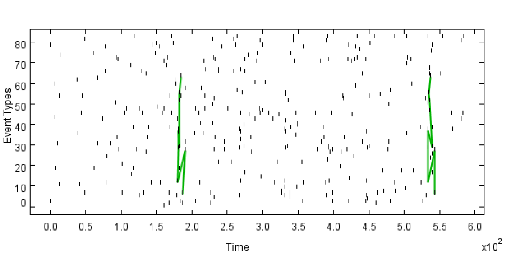

In this section we describe results obtained on calcium imaging data reported in [6]. (We are grateful to Dr. Rafeal Yuste for sharing this Calcium Imaging data with us). In [6], Ikegaya et. al. analyzed how neural activity propagates through cortical networks. They found precise repetitions of spontaneous patterns. These patterns repeated after minutes maintaining millisecond accuracy. In Fig. 3A of [6], such patterns are shown in raster plots by connecting the spikes that are part of an occurrence.
In Fig. 6, we show results obtained on the same calcium imaging data set using frequent episode discovery algorithms. Fig. 6 (a) shows two occurrences of a 10-node parallel episode discovered with expiry time constraint time units. Fig. 6 (b) shows four occurrences of two 4-node serial episode discovered with inter-event constraint of 0 to 10 time units. It is seen that the results obtained using frequent episode discovery match with those presented in [6]. Also, the time needed by our algorithm is much smaller because in [6], they use a counting technique that cannot control the combinatorial explosion. This result brings out the utility of our data mining technique in terms of both effectiveness and efficiency.
VI Conclusion
Frequent episode discovery is a very efficient temporal data mining technique. In this paper we have presented some new algorithms for frequent episode discovery under expiry time and inter-event time constraints. The temporal constraints are motivated by the problem of analyzing multi-neuron spiking data. We have discussed the kind of patterns that neurobiologists look for in such data and have shown that our algorithms are very effective in unearthing the underlying connectivity structure from spike data. In this context, our temporal constraints are very useful in focusing the search for patterns and tackling combinatorial explosion. Also, we can readily relate these constraints to relevant biological parameters.
One of the main motivations for this paper is to introduce the problem multi-neuron spike data analysis to data mining community. This is a challenging problem of analyzing large data sets to find underlying patterns, though no data mining techniques have so far been used for this. One can think of this problem as one of learning network connectivity pattern given only node-level dynamic data. Such a problem would be relevant in many other application areas as well. For example, analyzing abnormal behavior of communication networks, finding hidden causative chains in complex manufacturing processes controlled by distributed controllers, etc. We hope our results presented here would contribute towards developing of data mining techniques relevant in such applications.
References
- [1] M. Abeles and I. Gat. Detecting precise firing sequences in experimental data. J Neurosci Methods, 107(1-2):141–154, May 2001.
- [2] M. Abeles and G. L. Gerstein. Detecting spatiotemporal firing patterns among simultaneously recorded single neurons. J Neurophysiol, 60(3):909–924, Sep 1988.
- [3] R. Agrawal and R. Srikant. Mining sequential patterns. In P. S. Yu and A. S. P. Chen, editors, Eleventh International Conference on Data Engineering, pages 3–14, Taipei, Taiwan, 1995. IEEE Computer Society Press.
- [4] E. N. Brown, R. E. Kass, and P. P. Mitra. Multiple neural spike train data analysis: state-of-the-art and future challenges. Nat Neurosci, 7:456–461, May 2004. 10.1038/nn1228.
- [5] T. Hosoya, S. A. Baccus, and M. Meister. Dynamic predictive coding by the retina. Nature, 436(7047):71–77, Jul 2005.
- [6] Y. Ikegaya, G. Aaron, R. Cossart, D. Aronov, I. Lampl, D. Ferster, and R. Yuste. Synfire chains and cortical songs: temporal modules of cortical activity. Science, 304(5670):559–564, Apr 2004.
- [7] S. Laxman. Discovering Frequent Episodes: Fast algorithms, connection with HMMs and generalization. PhD thesis, Indian Institute of Science, March 2006.
- [8] S. Laxman and P.S.Sastry. A survey of temporal data mining. SADHANA, Academy Proceedings in Engineering Sciences, 2005.
- [9] S. Laxman, P.S.Sastry, and K. Unnikrishnan. Discovering frequent episodes and learning hidden markov models: A formal connection. IEEE Transactions on Knowledge and Data Engineering, 17(11):1505–1517, 2005.
- [10] A. K. Lee and M. A. Wilson. A combinatorial method for analyzing sequential firing patterns involving an arbitrary number of neurons based on relative time order. J Neurophysiol, 92(4):2555–2573, 2004.
- [11] H. Mannila, H. Toivonen, and A. Inkeri Verkamo. Discovery of frequent episodes in event sequences. Data Mining and Knowledge Discovery, 1:259–289, September 1997. doi:10.1023/A:1009748302351.
- [12] I. V. Tetko and A. E. Villa. A pattern grouping algorithm for analysis of spatiotemporal patterns in neuronal spike trains. 1. detection of repeated patterns. J Neurosci Methods, 105(1):1–14, Jan 2001.
- [13] D. A. Wagenaar, J. Pine, and S. M. Potter. An extremely rich repertoire of bursting patterns during the development of cortical cultures. BMC Neuroscience, 2006.