Untangling a Planar GraphThanks: This paper is based on two preliminary versions; (a) X. Goaoc, J. Kratochvíl, Y. Okamoto, Ch.-S. Shin, and A. Wolff: “Moving Vertices to Make Drawings Plane”, Proc. 15th International Symposium on Graph Drawing (GD’07), volume 4875 of Lecture Notes in Computer Science, pages 101–112, Springer-Verlag 2008, and (b) A. Spillner and A. Wolff: “Untangling a Planar Graph”, Proc. 34th International Conference on Current Trends in Theory and Practice of Computer Science (SOFSEM’08), volume 4910 of Lecture Notes in Computer Science, pages 473–484, Springer-Verlag 2008. Our work was started at the 9th “Korean” Workshop on Computational Geometry and Geometric Networks organized by A. Wolff and X. Goaoc, July 30–August 4, 2006 in Schloss Dagstuhl, Germany. Further contributions were made at the 2nd Workshop on Graph Drawing and Computational Geometry organized by W. Didimo and G. Liotta, March 11–16, 2007 in Bertinoro, Italy.
Abstract
A straight-line drawing of a planar graph need not be plane, but can be made so by untangling it, that is, by moving some of the vertices of . Let denote the minimum number of vertices that need to be moved to untangle . We show that is NP-hard to compute and to approximate. Our hardness results extend to a version of 1BendPointSetEmbeddability, a well-known graph-drawing problem.
Further we define to be the maximum number of vertices of a planar -vertex graph that can be fixed when untangling . We give an algorithm that fixes at least vertices when untangling a drawing of an -vertex graph . If is outerplanar, the same algorithm fixes at least vertices. On the other hand we construct, for arbitrarily large , an -vertex planar graph and a drawing of with and an -vertex outerplanar graph and a drawing of with . Thus our algorithm is asymptotically worst-case optimal for outerplanar graphs.
Keywords: Graph drawing, straight-line drawing, planarity, NP-hardness, hardness of approximation, moving vertices, untangling, point-set embeddability.
1 Introduction
A drawing of a graph maps each vertex of to a distinct point of the plane and each edge to an open Jordan curve connecting the images of and . A drawing of is plane if no two distinct edges cross, that is, intersect. By the famous theorem of Wagner [Wag36], Fáry [Fár48], and Stein [Ste51], any planar graph admits a plane straight-line drawing, that is, a drawing that maps edges to straight-line segments. Obviously not every straight-line drawing of a planar graph is plane. In this paper we are exclusively interested in such straight-line drawings. Thus by a drawing we will always mean a straight-line drawing. Since a (straight-line) drawing is completely defined by the position of the vertices, moving a vertex is a natural operation to modify such a drawing. If a drawing is to be made plane—or untangled—by successively moving vertices, it is desirable to move as few vertices as possible. The smaller the number of moves, the less likely it is that an observer gets confused, that is, the more likely the observer’s mental map [MELS95] is preserved during a sequence of changes. A recreational version of the problem of minimizing the number of moves is given by Tantalo’s popular on-line game Planarity [Tan07], where the aim is to untangle a straight-line drawing as quickly as possible, again by vertex moves. Actually, in Tantalo’s game an additional difficulty for the player is the fixed size of the screen; Liske’s [Lis08] version of the game allows rescaling and hence is fully equivalent to untangling.
We define the vertex-shifting distance between two drawings and of a graph to be the number of vertices of whose images under and differ:
Given our edit operation, represents the edit distance for straight-line drawings of graphs (see Fig. 1 for an example). For a drawing of a planar graph , we denote by the minimum number of vertices that need to be moved in order to untangle . In some sense measures the distance of from planarity. This suggests the following computational problem.
MinShiftedVertices: given a drawing of a planar graph , find a plane drawing of with .
The symmetric point of view is often helpful. Therefore we denote by the maximum number of vertices that can be fixed when untangling ; we refer to such vertices as fixed vertices. Clearly, , where is the number of vertices of . We call the corresponding problem, that is, finding a plane drawing of a given planar graph that maximizes the number of fixed vertices with a given drawing , MaxFixedVertices. We denote by the minimum of over all drawings of . Analogously, we denote by the maximum of over all drawings of .

Kaufmann and Wiese [KW02] considered the graph-drawing problem 1BendPointSetEmbeddability that will turn out to be related to MinShiftedVertices. They defined a planar graph to be -bend embeddable if, for any set of points in the plane, there is a one-to-one correspondence between and that can be extended to a plane drawing of with at most bends per edge. Kaufmann and Wiese showed that (a) every four-connected planar graph is 1-bend embeddable, (b) every planar graph is 2-bend embeddable, and (c) given a planar graph and set of points on a line, it is NP-complete to decide whether there is a correspondence between and that makes it possible to 1-bend embed on .
The contributions we present in this paper are three-fold:
- •
We prove that the decision versions of MaxFixedVertices and MinShiftedVertices are NP-hard (Theorem 3.1) and lie in (Proposition 3.7). We further prove that MinShiftedVertices is hard to approximate in the following sense: if there is a real and a polynomial-time algorithm that guarantees to untangle any drawing of any -vertex planar graph with at most moves, then (Theorem 3.3).
- •
We complement the complexity result of Kaufmann and Wiese [KW02] on 1BendPointSetEmbeddability by showing that it is NP-hard to decide whether a given one-to-one correspondence between the vertices of a planar graph and a planar point set extends into a plane drawing of with at most one bend per edge (Theorem 3.4). We also show that the problem lies in (Theorem 3.6) and that an optimization version of the problem is hard to approximate (Corollary 3.5).
- •
We show that for any -vertex outerplanar graph (Corollary 4.9) and that for any general planar graph with vertices (Theorem 4.11), where the base of logarithms is . We also give, for arbitrarily large , examples of an -vertex outerplanar graph with (Theorem 6.1) and of an -vertex planar graph with (Theorem 5.3). We prove the two bounds by using drawings where all vertices lie on a line.
2 Previous and Related Work
Arguably, one of the earliest results on untangling, for the -path in the real line, is the Erdős–Szekeres theorem, which we state here for further reference.
Theorem 2.1 (Erdős and Szekeres [ES35]).
Any sequence of different real numbers has an increasing subsequence of terms or a decreasing subsequence of terms.
The current best bounds on , where is restricted to certain classes of planar graphs, are summarized in Table 1. Recall that a lower bound of means that we can untangle any drawing of any -vertex graph in the given graph class while fixing at least vertices, whereas an upper bound of means that for arbitrarily large there exists a drawing of an -vertex graph in the given graph class such that at most vertices can stay fixed when untangling .
| Graph class | Lower bound | Upper bound | ||
|---|---|---|---|---|
| Cycles | [Cib08] | [PT02] | ||
| Trees | [BDH+08] | [BDH+08] | ||
| Outerplanar graphs | [RV08] & Corollary 4.9 | Theorem 6.1 | ||
| Planar graphs | [BDH+08] | Theorem 5.3 | ||
Untangling was first investigated for the -cycle , following the question by Watanabe [Wat98] of whether . The answer turned out to be negative: Pach and Tardos [PT02] showed, by a probabilistic argument, that . They also showed that by applying the Erdős–Szekeres theorem to the sequence of the indices of the vertices of in clockwise order around some specific point. Cibulka [Cib08] recently improved that lower bound to by applying the Erdős–Szekeres theorem not once but times.
Pach and Tardos [PT02] extended the question to planar graphs and asked whether there is a constant such that for any planar -vertex graph . This question was recently answered in the affirmative by Bose et al. [BDH+08], who showed that . While their bound improves on our Theorem 4.11, their algorithm uses our algorithm as a subroutine (specifically the result in Corollary 4.9). A recent improvement in our analysis also improves their bound, yielding . Kang et al. [KPR+08] showed that for arbitrarily large there is a planar graphs with vertices and fix. For our upper bound of , see Theorem 5.3. Kang et al. [KPR+08] also shed some light on how upper bounds on are affected by restricting the possible locations of vertices in the drawings of . In particular, they showed that initial drawings with all vertices on a line, such as our examples in Theorems 6.1 and 5.3, are the worst case in the sense that any planar graph has such a drawing with , and that their upper bound holds even in the case where initial drawings are restricted to drawings where vertices correspond to a set of points on the boundary of a convex set. (Note that this generalizes both the vertices-on-a-line case and the vertices-in-convex-position case.)
Verbitsky [Ver08] investigated planar graphs of higher connectivity. He proved linear upper bounds on for three- and four-connected planar graphs. Cibulka [Cib08] gave, for any planar graph , an upper bound on that is a function of the number of vertices, the maximum degree, and the diameter of . This latter bound implies, in particular, that for any three-connected planar graph and that any graph such that for some must have a vertex of degree .
For the class of trees, Bose et al. [BDH+08] showed that for any tree with vertices. They further showed that for a collection of stars with vertices in total, which, up to adding one vertex to turn these stars into a single tree, implies that the previous bound is asymptotically tight. We have obtained the same lower bound of for the larger class of outerplanar graphs (Corollary 4.9). This bound was obtained independently by Ravsky and Verbitsky [RV08] via a finer analysis of sets of collinear vertices in plane drawings.
The hardness of computing given and was obtained independently by Verbitsky [Ver08] by a reduction from independent set in line-segment intersection graphs. While our proof is more complicated than his, it is stronger as it also yields hardness of approximation and extends to the problem 1BendPointSetEmbeddability with given vertex–point correspondence.
Finally, a somewhat related problem is that of morphing, or isotopy, between two plane drawings and of the same graph , that is, to define for each vertex of a movement from to such that at any time during the move the drawing defined by the current vertex positions is plane. We refer the interested reader to the survey by Lubiw et al. [LPS06].
3 Complexity
In this section, we investigate the complexity of MinShiftedVertices and of 1BendPointSetEmbeddability with given vertex–point correspondence.
Theorem 3.1.
Given a planar graph , a drawing of , and an integer , it is NP-hard to decide whether .
Proof.
Our proof is by reduction from Planar3SAT, which is NP-hard [Lic82]. An instance of Planar3SAT is a 3-SAT formula whose variable-clause graph is planar. Note that this graph can be laid out (in polynomial time) such that variables correspond to rectangles centered on the -axis and clauses correspond to non-crossing three-legged “combs” completely above or completely below the -axis [KR92], see Fig. 2. We refer to this layout of the variable-clause graph as . We now construct a graph with a straight-line drawing such that the following holds: can be untangled by moving at most vertices if and only if is satisfiable. We fix later.

Our graph consists of two types of substructures (or gadgets), modeling the variables and clauses of . The overall layout of follows (see Fig. 2): the variable gadgets are drawn in the same order along the -axis as the variable nodes in , and the clause gadgets form non-crossing three-legged combs that lie on the same side of the -axis as the corresponding clause nodes in .
In our gadgets, see Figs. 3 and 4, there are two types of vertices and edges; those that may move and those that are meant not to move. We refer to the two types as mobile and immobile. Each mobile vertex (but no immobile vertex) is incident to two edges that cross two other edges. The drawing that we specify in the following has crossings; if has a satisfying truth assignment, can be untangled by moving mobile vertices. Otherwise, at least one immobile vertex must move, and thus in total at least vertices need to move. In the figures, immobile vertices are marked by black disks, mobile vertices by circles, and their predestined positions by little squares. Mobile edges—edges incident to a mobile vertex—are drawn as thick solid gray line segments, and their predestined positions as gray line segments that are dashed, dotted, or dashed-dotted (and thus not solid). Immobile edges are drawn as solid black line segments.
Now consider the gadget for some variable in , see the shaded area in Fig. 3.

The gadget consists of a horizontal chain of a certain number of roughly square blocks. Each block consists of 28 vertices (four of which are mobile) and 28 edges. In Fig. 3 the four mobile vertices of the leftmost block are labeled in clockwise order , , , and . Note that the gray edges incident to and intersect those incident to and . Thus either both and or both and must be moved to untangle the block. Each mobile vertex can move into exactly one position (up to small perturbations). The resulting incident edges are drawn by dotted and dashed gray line segments, respectively. Note that neighboring blocks in the chain are placed such that the only way to untangle them simultaneously is to move corresponding pairs of vertices and edges. Thus either all blocks of a variable gadget use the dashed line segments or all use the dotted line segments. These two ways to untangle a variable gadget correspond to the values true and false of the variable, respectively.
Let be the numbers of clauses of . For each of the literals in we connect the gadget of the corresponding variable to the gadget of the clause that contains the literal. Each block of each variable gadget is connected to a specific clause gadget above or below the variable gadget, thus there are blocks in total. Each connection is realized by a part of that we call a 2-switch. A 2-switch consists of 15 vertices and 14 edges. The mobile vertex of the 2-switch in Fig. 3 is incident to two thick gray edges that intersect two immobile edges of the 2-switch. Thus must move. There are (up to small perturbations) two possible positions, namely and , see Fig. 3.
The 2-switch in Fig. 3 corresponds to a positive literal. For negated literals the switch must be mirrored either at the vertical or at the horizontal line that runs through the point . Note that a switch can be stretched vertically in order to reach the right clause gadget. Further note that if a literal is false, the mobile vertex of the corresponding 2-switch must move away from the variable gadget and towards the clause gadget to which the 2-switch belongs. In that case we say that the 2-switch transmits pressure.
A clause gadget consists of three vertical 2-switches and two horizontal 3-switches. A 3-switch consists of 23 vertices and 18 edges plus a small “inner” 2-switch, see the shaded area in Fig. 4.

Independently from the other, each of the two 3-switches can be stretched horizontally in order to reach vertically above the variable gadget to which it connects via a 2-switch. The mobile vertex of the left 3-switch in Fig. 4 is incident to two thick gray edges that intersect two immobile edges of the 3-switch. Thus must move. There are (again up to small perturbations) three possible positions, namely , , and . Note that we need the inner 2-switch, otherwise there would be a forth undesired position for moving , namely the one labeled in Fig. 4. By construction, a clause gadget can be made plane by only moving the mobile vertices of all switches if and only if at most two of the three big 2-switches transmit pressure, that is, if at least one of the literals in the clause is true.
The graph that we have now constructed has vertices, edges, and crossings; in blocks and in switches. Recall that any mobile vertex is incident to two edges that each cross another edge. Thus a mobile vertex corresponds to a pair of crossings. By moving a mobile vertex to any of its predestined positions, the corresponding pair of crossings disappears. If is satisfiable, can be made plane by moving mobile vertices since no new crossings are introduced. If is not satisfiable, there is at least one pair of crossings that cannot be eliminated by moving the corresponding mobile vertex alone since all its predestined positions are blocked. Thus at least two vertices must be moved to eliminate that pair of crossings—and still all the other pairs of crossings must be eliminated by moving at least one vertex per pair, totaling in at least moves. Thus is satisfiable if and only if can be made plane by moving exactly (mobile) vertices.
Recall that consists of vertices and edges. We construct step by step, starting with the vertices of the variable gadgets and then treating the clauses from innermost to outermost. In order for the 2- and 3-switches to reach far enough, note that each desired position of a mobile vertex is determined by two pairs of immobile vertices. By making the distances of the two vertex pairs (polynomially) small, the desired position can be confined to a region that is small enough to force the mobile vertex of the next switch into one of its remaining positions. Now it is clear that it is possible to place vertices at coordinates whose representation has size polynomial in the length of a binary encoding of . This implies that our reduction is polynomial in . ∎
Remark 3.2.
Our proof can be slightly modified to show that the problem is also hard if we are additionally given an axis-parallel rectangle that contains the initial graph drawing, and each move is constrained to that rectangle—in other words Tantalo’s version of the planarity game. In the proof we simply compute from the given planar 3-SAT formula a rectangle that is large enough to accommodate not only the initial drawing, but also the plane drawing that we get in case the formula has a satisfying truth assignment. Note that this rectangle is barely larger than the smallest axis-parallel rectangle that contains all vertices of our initial graph drawing.
We now consider the approximability of MinShiftedVertices. Since for plane drawings, we cannot use the usual definition of an approximation factor unless we slightly modify our objective function. Let and call the resulting decision problem MinShiftedVertices′. Now we can modify the above reduction to get a non-approximability result.
Theorem 3.3.
For any constant real there is no polynomial-time -approximation algorithm for MinShiftedVertices′ unless .
Proof.
Let be the number of vertices of the graph with drawing that we constructed above. We add to for each edge copies, half of them on each side of , in the close vicinity of . If one of the endpoints of is a mobile vertex, then all copies are incident to that vertex. In the following we detail where to place the other (new) endpoints of these edges.
We go through each immobile vertex of . Let be the degree of in . Note that . If , we place the endpoints of the copies of the edge incident to on the two rays that are orthogonal to in . On each ray we place half of the endpoints and connect them by new edges along the ray, starting with , see vertex in Fig. 5.
Otherwise, if , let , be two edges that are incident to and consecutive in the circular ordering around . Now we add half of the endpoints of and on a ray between and emanating from , in the same manner as above. The position of the ray depends on whether both and are immobile or one of them is mobile. (Being immobile, vertex is incident to at most one mobile edge.) In the first case we place the new vertices on the angular bisector of and , see vertex in Fig. 5. In the second case where one of the edges, say , is mobile, note that the original and all predestined positions of lie in an open halfplane bounded by a line through . So we place the new vertices on , half on each side of , see vertex in Fig. 5.
Let be the resulting graph, its drawing, and the number of vertices of . Note that is satisfiable if and only if . Otherwise, in the original graph at least one immobile vertex has to move. This vertex either is incident to a mobile edge or it is not, see Fig. 4(b) and (c), respectively. In the new graph , which contains , also at least one (original) immobile vertex has to move. If is not incident to a mobile edge, in order to make space, all new vertices in the vicinity of have to move, too. If is incident to a mobile edge, a new vertex in the vicinity of has to move only if it is incident to a new copy of the mobile edge. That is, in both cases, at least vertices have to move. In other words, . Note that can be constructed in polynomial time since we have assumed to be a constant.

Suppose there was a polynomial-time -approximation algorithm for MinShiftedVertices′. We can bound its approximation factor by . Now let be the number of moves that needs to untangle . If is satisfiable, then . On the other hand, if is unsatisfiable, then . Since we can assume that is sufficiently large, the result of algorithm (that is, the number ) tells us whether is satisfiable. So either our assumption concerning the existence of is wrong, or we have shown the NP-hard problem Planar3SAT to lie in , which in turn would mean that . ∎
We now state a hardness result that establishes a connection between MinShiftedVertices and the well-known graph-drawing problem 1BendPointSetEmbeddability. We define the problem 1BendPointSetEmbeddabilityWithCorrespondence as follows. Given a planar graph , a set of points in the plane with rational coordinates and a one-to-one correspondence between and , decide whether can be extended to a plane 1-bend drawing of , that is, whether has a plane drawing such that for all and such that maps each edge of to a 1-bend polygonal chain.
Theorem 3.4.
1BendPointSetEmbeddabilityWithCorrespondence is NP-hard.
Proof.
The proof uses nearly the same gadgets as in the proof of Theorem 3.1: set to a copy of where each length-2 path containing a mobile vertex is replaced by the edge . We refer to this type of edges as new edges. The vertices of are mapped to the corresponding vertices in . We claim that has a 1-bend drawing if and only if the given planar-3SAT formula is satisfiable.
In order to see that the claim holds, note the two differences to the proof of Theorem 3.1. First, in 1BendPointSetEmbeddabilityWithCorrespondence all vertices are fixed. This makes it even easier to argue correctness. Second, any edge can bend, not only new edges, which are meant to bend. Due to the fact that vertices cannot move, however, all groups of edges that are meant to be obstacles will remain obstacles to the bending of the new edges. The only way to embed the new edges is to route them around the obstacles exactly as in Figs. 3 and 4(a). ∎
Now suppose that we already know that has a plane drawing with at most one bend per edge. Then it is natural to ask for a drawing with as few bends as possible. Let be 1 plus the minimum number of bends over all plane 1-bend drawings of . The following corollary shows that it is hard to approximate efficiently.
Corollary 3.5.
Given a planar graph , a set , a one-to-one correspondence between and that can be extended to a plane 1-bend drawing of , and a constant , it is NP-hard to approximate within a factor of .
Proof.
We slightly change the clause gadget in the proof of Theorem 3.4. Apart from the three vertical 2-switches, the clause gadget now consists of two 4-switches and of two stacks of edges each, see Fig. 6. Let be the resulting graph, which depends on the given planar 3SAT formula . The 4-switches make sure that always has a drawing with at most one bend per edge. Each stack is placed in the vicinity of a 4-switch such that all stack edges have to bend if the central switch edge is forced to bend into the direction of the stack. (In Fig. 6, the central switch edges in the left and right 4-switch are labeled and , respectively.) If is not satisfiable, at least one clause evaluates to false and in the corresponding gadget all edges in the left or all edges in the right stack need to bend.

We do not know whether 1BendPointSetEmbeddabilityWithCorrespondence or MinShiftedVertices lie in , but it is not hard to show the following.
Theorem 3.6.
1BendPointSetEmbeddabilityWithCorrespondence is in .
Proof.
Let be a planar graph, a set of points in the plane with rational coordinates, and a one-to-one correspondence between and . Any 1-bend drawing of that extends is uniquely determined by choosing, for each edge , the position of the bend of . (If an edge is to be drawn without bend, any point in the relative interior of the line segment connecting and can be chosen.) Thus, the set of all plane 1-bend drawings of that extend can be represented by a subset of . The bend splits (the drawing of) the edge into two relative open line segments to which we refer as half-edges.
In order to decide the existence of a plane 1-bend drawing, we specify a predicate in polynomial inequalities with integer coefficients and with variables in the set . We do this by first expressing the condition that no two half-edges with distinct endpoints may intersect. Given four distinct points , , , and , the requirement that points and lie in different half-planes determined by the line through and can be expressed by an inequality , where is a degree-4 polynomial with integer coefficients and with variables representing the coordinates of the four points [KM94]. The requirement that the line segments and are disjoint is described by the disjunction .
Second, we add conditions that guarantee that no bend coincides with a point in , that all bends are distinct, and that no two half-edges overlap if they share an endpoint. All these conditions can also be described as Boolean combinations of polynomial inequalities with integer coefficients and with variables from . As a consequence, deciding whether extends to a 1-bend drawing of recasts into deciding the non-emptiness of a set in defined by a predicate whose atomic formulas are polynomial inequalities with integer coefficients, a problem that is in [Can88, Ren92]. ∎
For MinShiftedVertices and MaxFixedVertices an additional trick is needed.
Proposition 3.7.
MinShiftedVertices and MaxFixedVertices are in .
Proof.
Obviously, both problems have the same optimal solutions, so it is enough to treat one of them, say MinShiftedVertices. We build on the formulation sketched in the proof of Theorem 3.6. Additionally, we introduce a binary variable for each vertex that encodes whether we move vertex () or not (). In order to restrict to these two values, we introduce the quadratic equation . The -coordinate of vertex in the plane target drawing can then be described by , where is the original -coordinate of and is the -coordinate of after a possible movement. The -coordinate of is treated analogously. The intersection of edges can be expressed as in the proof of Theorem 3.6. To bound the number of moved vertices by , we introduce the inequality . ∎
4 Planar Graphs: Lower Bound
Any drawing of a planar graph with vertices, other than or , can be untangled while fixing at least three vertices [Ver08]. In this section, we give an algorithm proving that
for any planar graph with vertices. Note that actually grows, albeit very slowly: only for some . Partially building on our algorithm, Bose et al. [BDH+08] showed that , a bound greater than for .
We first give some definitions (Section 4.1) and sketch the basic idea of our algorithm (Section 4.2). Then we describe our algorithm (Section 4.3) and prove its correctness (Section 4.4). The bound depends on finding a plane embedding of that contains a long simple path with an additional property. We show how to find such an embedding in Section 4.5.
4.1 Definitions and notation
Recall that a plane embedding of a planar graph is given by the circular order of the edges around each vertex and by the choice of the outer face. A plane embedding of a planar graph can be computed in linear time [HT74]. If is triangulated, a plane embedding of is determined by the choice of the outer face. Further recall that an edge of a graph is called a chord with respect to a path (or cycle) if the edge does not lie on but both its endpoints are vertices of .
For a point , let and be the - and -coordinates of , respectively. We say that lies vertically below if and . For a polygonal path , we denote by the set of vertices of and by the set of edges of . We call a polygonal path -monotone if . In addition, we say that a point lies below an -monotone path if lies vertically below a point (not necessarily a vertex!) on . Analogously, a line segment lies below if every point lies below . We do not always strictly distinguish between a vertex of and the point to which this vertex is mapped in a particular drawing of . Similarly, we write both for the edge of and the straight-line segment connecting with .
4.2 Basic idea
Note that in order to establish a lower bound on , we can assume that the given graph is triangulated. Otherwise we can triangulate arbitrarily (by fixing an embedding of and adding edges until all faces are 3-cycles) and work with the resulting triangulated planar graph. A plane drawing of the latter yields a plane drawing of . So let be a triangulated planar graph, and let be any drawing of . It will also be convenient to assume that in the given drawing , the vertices of are mapped to points with pairwise distinct -coordinates. By slightly rotating the drawing we can always achieve this.
The basic idea of our algorithm is to find a plane embedding of such that there exists a long simple path connecting two vertices and of the outer triangle with the property that all chords of lie on one side of (with respect to ) and lies on the other. For an example of such an embedding , see Fig. 7(b). We describe how to find and depending on the maximum degree and the diameter of in Section 4.5. For the time being, we assume they are given. Now our goal is to produce a drawing of according to the embedding and at the same time keep many of the vertices of at their positions in . Having all chords on one side is the crucial property of that we use to achieve this. We allow ourselves to move all other vertices of to any location we like, a process we will occasionally refer to as drawing certain subgraphs of . This gives us a lower bound on in terms of the number of vertices of . Our method is illustrated in Fig. 7; we give the details in the next subsection.
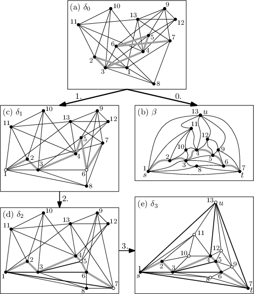
4.3 Description of the algorithm
Let denote the set of chords of . We assume that these chords lie to the right of when we traverse this path from to in the embedding . (Note that “below” is not defined in an embedding.) Let denote the set of vertices of that lie to the right of in and let . Note that lies in . Let be a subset of the vertices of such that no two vertices in are connected by a chord of . We will choose such that , and our method tries to fix many of the vertices in .
In step 1 of our algorithm we move some of the vertices in from the position they have in to new positions such that the resulting ordering of the vertices in according to increasing -coordinates is the same as the ordering along in . This yields a new (usually non-plane) drawing of that maps on an -monotone polygonal path . By Theorem 2.1 we can choose such that at least of the vertices in remain fixed. Let be the set of the fixed vertices. Note that for all , see Fig. 7(c).
Once we have constructed , we have to find suitable positions for the vertices in . This is simple for the vertices in : if we move vertex , which lies on the outer face, far enough above , then the polygon bounded by and by the edges and will be star-shaped. Recall that a polygon is called star-shaped if the interior of its kernel is non-empty, and the kernel of a clockwise-oriented polygon is the intersection of the right half-planes induced by the edges of . Now if is star-shaped, we have fulfilled one of the assumptions of the following result of Hong and Nagamochi [HN08] for drawing triconnected graphs, that is, graphs that cannot be disconnected by removing two vertices. We will use their result in order to draw into the subgraph of induced by excluding the chords in .
Theorem 4.1 ([HN08]).
Given a triconnected plane graph , every drawing of the outer facial cycle of on a star-shaped polygon can be extended in linear time to a plane drawing of .
Observe, however, that is not necessarily triconnected: vertex may be adjacent to vertices on other than and . In order to fix this, we split into smaller units along the edges incident to . Let be the sequence of vertices of . Let be a pair of integers such that , vertices and are adjacent to and any vertex with is not adjacent to . Consider the subgraph of induced by the vertices that lie (with respect to ) inside of or on the cycle . In the following we convince ourselves that this subgraph is actually triconnected. Let be the family of all such subgraphs.
Recall that a planar graph is called a rooted triangulation [Avi96] if in every plane drawing of there exists at most one facial cycle with more than three vertices. According to Avis [Avi96], the following lemma is well known.
Lemma 4.2 ([Avi96]).
A rooted triangulation is triconnected if and only if no facial cycle has a chord.
Now it is clear that we can apply Theorem 4.1 to draw each of the subgraphs in . By the placement of , each drawing region is star-shaped, and by construction, each subgraph is chordless and thus triconnected. However, to draw the graph induced by (including the chords in ), we must work a little harder.
In step 2 of our algorithm we once more change the drawing of . Let . Note that every chord of has at least one of its endpoints in . Now we go through the vertices in in a certain order, moving each vertex vertically down as far as necessary (see vertices 5 and 7 in Fig. 7(d)) to achieve two goals: (a) all chords in move below the resulting polygonal path , and (b) the faces bounded by , the edge , and the chords become star-shaped polygons. This defines a new drawing , which leaves all vertices in and all vertices in fixed.
In step 3 we use the fact that is still -monotone. This allows us to move vertex to a location above where it can see every vertex of . Now , the edges of type (with ) and the chords in partition the triangle into star-shaped polygons with the property that the subgraphs of that have to be drawn into these polygons are all rooted triangulations, and thus triconnected. This means that we can apply Theorem 4.1 to each of them. The result is our final—and plane—drawing of , see Fig. 7(e).
4.4 Correctness of the algorithm
We now show that our algorithm indeed produces a plane drawing where many of the vertices on the chosen path are fixed. To this end, recall that is the set of vertices in we fixed in step 1, that is, in the construction of the -monotone polygonal path . Our goal is to fix the vertices in when we construct , which also is an -monotone polygonal path but has two additional properties: (a) all chords in lie below and (b) the faces induced by , , and the chords in are star-shaped polygons. The following lemmas form the basis for the proof of the main theorem of this section (Theorem 4.7), which shows that this can be achieved.
Lemma 4.3.
Let be an -monotone polygonal path such that (i) the segment lies below and (ii) the polygon bounded by and is star-shaped. Let be any point vertically below . Then the polygon is also star-shaped.
Proof.
Only two edges change when we move vertex to its new position , namely and . Consider the remaining edges that do not change and let be the intersection of the corresponding right half-planes. Since the edges form an -monotone path, is not bounded. Let be a point in the interior of the kernel of . Then lies in the interior of and, moreover, every point that is vertically below also lies in the interior of . Let be a point vertically below and sufficiently close to the edge . Then lies in the interior of the kernel of , and therefore is star-shaped by definition. ∎
Lemma 4.4.
Let be an -monotone polygonal path, and let be a set of pairwise non-crossing straight-line segments with endpoints in that all lie below . Let be a point vertically below , let , and finally let be a copy of with each segment replaced by .
Then the segments in are pairwise non-crossing and all lie below .
Proof.
Let be the straight-line segments incident to (both on the monotone path and in ), sorted clockwise around such that . Note that, since the straight-line segments in are below , the vertices are also sorted according to increasing -coordinates, and all of them have smaller -coordinate than . Hence, the situation is as depicted in Fig. 8.

For , let denote the set of points that lie below the straight-line segment and define , see the shaded region in Fig. 8. Note that the interior of cannot contain any vertices of since this would contradict the fact that is -monotone or the fact that all straight-line segments in are below . But this implies that none of the straight-line segments (drawn dotted in Fig. 8) is crossed by a straight-line segment in since this would yield a contradiction to the fact that the straight-line segments in are non-crossing or to the fact that the interior of does not contain a vertex of . No other crossings can occur in since the straight-line segments in are non-crossing. This finishes the proof. ∎
Recall that we aim at finding a large set such that no two vertices in are connected by a chord of . The set of fixed vertices will be a subset of . Note that may contain vertices connected by an edge of . In the following lemma, the set contains all vertices of that we have to move in order to draw the chords of straight-line; clearly such a set must cover all chords of . Thus the set plays the role of the complement of .
Lemma 4.5.
Let be an -monotone polygonal path. Let be a set of chords of that can be drawn as non-crossing curved lines below . Let be a vertex cover of . Then there is a way to modify by decreasing the -coordinates of the vertices in such that the resulting straight-line drawing of is plane, the bounded faces of are star-shaped, and all edges in lie below the modified polygonal path, which is also -monotone. The coordinates of the vertices of the modified path have bit length , where is the maximum bit length of the vertex coordinates of .
Proof.
We use induction on the number of chords. If , we need not modify . So, suppose that . We first choose a chord with such that there is no other edge with the property that and . Clearly, such an edge always exists. Then we apply the induction hypothesis to . This yields a modification of such that is -monotone, all edges in the resulting straight-line drawing of lie below , and all bounded faces in this drawing are star-shaped.
Now consider the chord and, without loss of generality, assume that . Let denote the set of those vertices with the property that no point vertically below and distinct from is contained in an edge of the drawing . Note that, since is -monotone, there must exist a point vertically below such that for no vertex , the straight-line segment crosses any edge in the drawing of .
Let be such that . We move vertex to the point to obtain a new drawing of . Then we apply Lemma 4.4 to the rightmost vertex of the -monotone subpath of with vertices and, similarly, we apply Lemma 4.4 to the leftmost vertex of the -monotone subpath of with vertices . It follows that this does not produce any crossings among the edges in the drawing . Moreover, by our choice of the chord , for each face in the drawing of that has vertex in its facial cycle, must be the leftmost or the rightmost vertex in this facial cycle. Hence, we can apply Lemma 4.3 to these faces. This yields that they remain star-shaped in . By the choice of we ensure that the bounded face that results from adding the straight-line segment to the drawing is also star-shaped.
Concerning the size of the coordinates we argue as follows. Without loss of generality we can assume that all vertices of have negative -coordinates. Now consider the addition of the -th chord . Let be the minimum -coordinate of a vertex in the drawing before moving vertex down. Then it is not hard to check that, in order to add the chord without introducing any crossings, it suffices to move down to a point with -coordinate , where is the ratio of the maximum over the minimum difference between the -coordinates of any two distinct vertices in . Solving the recurrence for yields . Therefore, since there are only chords, the -coordinates in the resulting -monotone path can be encoded using bits. ∎
Remark 4.6.
Unfortunately, there are indeed instances where our algorithm actually needs bits for representing all -coordinates of the modified path. Let be an odd integer, and let be a path with vertices , where for and , see the thick light-gray path in Fig. 9. We set (drawn with dotted arcs in Fig. 9) and (marked with circles in Fig. 9).
Our algorithm straightens the chords in the order from innermost to outermost, that is, vertices are moved in the order . To simplify presentation, let denote the vertices of in this order, and let . For , denote the final position of by . Then clearly for . The edges incident to have slope (with the exception of the irrelevant edge ), thus . The recursion solves to .

Now suppose that we have modified the -monotone path according to Lemma 4.5. Then the resulting -monotone path admits a straight-line drawing of the chords in below such that the bounded faces are star-shaped polygons, see the example in Fig. 7(d). Recall that is the vertex of the outer triangle in that does not lie on . We now move vertex to a position above such that all edges with can be drawn without crossing and such that the resulting faces are star-shaped polygons. Since is -monotone, this can be done. As an intermediate result, we obtain a plane straight-line drawing of a subgraph of where all bounded faces are star-shaped. It remains to find suitable positions for the vertices in . For every star-shaped face , there is a unique subgraph of that must be drawn inside this face. Note that by our construction every edge of that has both endpoints on the boundary of must actually be an edge of the boundary. Therefore, is a rooted triangulation where no facial cycle has a chord. Now Lemma 4.2 yields that is triconnected. Finally, we can use the result of Hong and Nagamochi [HN08] (see Theorem 4.1) to draw each subgraph of type and thus finish our construction of a plane straight-line drawing of , see the example in Fig. 7(e). We summarize.
Theorem 4.7.
Let be a triangulated planar graph that contains a simple path and a face . If has an embedding such that is the outer face, lies on one side of , and all chords of lie on the other side, then .
Proof.
We continue to use the notation introduced earlier in this section. Recall that we aim at finding a large set such that no two vertices in are connected by a chord of . The complement of this set is the vertex cover of that we need for applying Lemma 4.5.
Further, is the set of vertices that we fixed in the first step, that is, in the construction of the -monotone path . It follows from Proposition 1 in the paper by Pach and Tardos [PT02] that we can make sure that . Consider the graph with vertex set and edge set . An independent set in has exactly the property that we want for . Thus it suffices to show that the -vertex graph has an independent set of size at least . We do this by giving a simple algorithm.
Our algorithm is greedy: we always take a vertex of smallest degree, put it in the independent set under construction, remove and the neighbors of from , and remove the edges incident to these vertices from . We repeat this until is empty.
Note that initially has at least one isolated (that is, degree-0) vertex, and that the bound is obvious if is a forest—the algorithm first picks all isolated vertices and then repeatedly picks leaves. Even if contains cycles, the algorithm always picks vertices of degree at most 2. This is due to the fact that all chords lie on one side of , and thus is and remains outerplanar, and any outerplanar graph has a vertex of degree at most 2.
Let be the number of vertices that have degree when they are put in . As observed above, . Whenever we put a vertex of degree into , we remove vertices from , thus . Let be the number of bounded faces of . Whenever the algorithm removes a degree-2 vertex, the number of bounded faces of decreases by one, thus . We claim—and will prove below—that . Now adding to the above expression for yields , or , which proves the theorem.
It remains to prove our claim, that is, . In other words, we need to show that contains at least one isolated vertex more than bounded faces. Recall that does not include the edges of . For a chord in , we define to be the span of . Now consider a face of with vertices and . The edges of are . Note that the span of contains the span of every other edge of . We define the span of to be the span of the edge .
We prove our claim by induction on . As noted above, contains at least one isolated vertex. This establishes the base of the induction. Now suppose that . Consider the set of all faces of whose span is maximal with respect to set inclusion. If , we apply the induction hypothesis to the subgraphs of induced by the spans of the faces in . Otherwise, let be the only face in , and let be the edges of whose span is properly contained in the span of . We apply the induction hypothesis to the subgraphs of induced by the spans of . Since , there are at least two such subgraphs. Each of them contains at least one isolated vertex more than bounded faces. Taking into account, we conclude that also contains at least one isolated vertex more than bounded faces. This completes the proof of our claim. ∎
4.5 Finding a Suitable Path
We finally present two strategies for finding a suitable path . Neither depends on the geometry of the given drawing of . Instead, they exploit the graph structure of . The first strategy works well if has a vertex of large degree and, even though it is very simple, yields asymptotically tight bounds for outerplanar graphs.
Lemma 4.8.
Let be a triangulated planar graph with maximum degree . Then .
Proof.
Let be a vertex of degree and consider a plane embedding of where vertex lies on the outer face. Since is planar, such an embedding exists. Let be the set of neighbors of sorted clockwise around in . This gives us the desired polygonal path that has no chords on the side that contains . Thus Theorem 4.7 yields . ∎
Lemma 4.8 yields a lower bound for outerplanar graphs that is asymptotically tight as we will see in Section 6.
Corollary 4.9.
Let be an outerplanar graph with vertices. Then .
Proof.
We select an arbitrary vertex of . Since is outerplanar, we can triangulate in such a way that in the resulting triangulated planar graph vertex is adjacent to every other vertex in . Thus the maximum degree of a vertex in is , and the result follows by Lemma 4.8. ∎
Our second strategy works well if the diameter of is large.
Lemma 4.10.
Let be a triangulated planar graph of diameter . Then .
Proof.
We choose two vertices and such that a shortest – path has length . We compute any plane embedding of that has on its outer face. Let and be the neighbors of on the outer face. Recall that a Schnyder wood (or realizer) [Sch89] of a triangulated plane graph is a (special) partition of the edge set into three spanning trees each rooted at a different vertex of the outer face. Edges can be viewed as being directed to the corresponding roots. The partition is special in that the cyclic pattern in which the spanning trees enter and leave a vertex is the same for all inner vertices. Schnyder [Sch89] showed that this cyclic pattern ensures that the three unique paths from a vertex to the three roots are vertex-disjoint and chordless. Let , , and be the “Schnyder paths” from to , , and , respectively. Note that the length of is at least , and the lengths of and are both at least . Let be the path that goes from along to and from along to . The length of is at least . Note that, due to the existence of , the path has no chords on the side that contains . Thus, Theorem 4.7 yields . ∎
Next we determine the trade-off between the two strategies above.
Theorem 4.11.
Let be a planar graph with vertices. Then , where the base of logarithms is .
Proof.
Let be an arbitrary triangulation of . Note that the maximum degree of is at least since and is triangulated. To relate to the diameter of , we use a very crude counting argument—Moore’s bound: starting from an arbitrary vertex of , we bound the number of vertices we can reach by a path of a certain length. Let be the smallest integer such that . Then . By the definition of we have , which we can simplify to since . Hence we have .
Remark 4.12.
The proof of Theorem 4.11 (together with the auxiliary results stated earlier) yields an -time algorithm for untangling a given straight-line drawing of a planar graph with vertices by moving some of its vertices to new positions. The first step, that is, computing the -monotone path , takes time [Sch61]. Moving the vertices of such that the faces induced by the path and its chords become star-shaped takes time (Lemma 4.5), where is an upper bound on the time needed to perform an elementary operation involving numbers of bit length . The remaining steps of our method can be implemented to run in time. This includes calling the algorithm of Hong and Nagamochi [HN08] and computing the Schnyder wood [Sch89], which we need in the proof of Lemma 4.10.
5 Planar Graphs: Upper Bound
We now give an upper bound for general planar graphs that is better than the upper bound of Pach and Tardos [PT02] for cycles. Our construction uses the following sequence, which we call and which we re-use in Section 6:
Note that can be written as , where is the subsequence of that consists of all numbers in that are congruent to modulo . To stress this, the last element in each of these subsequences is underlined in . Thus consists of distinct numbers. It is not hard to see the following.
Observation 5.1.
The longest increasing or decreasing subsequence of has length .
We call two subsequences and of separated if
- (i)
comes before or comes before in , and
- (ii)
or ).
Observation 5.2.
Let and be two separated decreasing or two separated increasing subsequences of . Then .
Proof.
First consider the case that and are both decreasing. Since they are separated we can assume without loss of generality that . We define for . Then, since and are both decreasing, they can each have at most one element in common with every . Now suppose that they have both one element in common with some . Then, since , cannot have an element in common with any , , and cannot have an element in common with any , . Therefore, .
If and are both increasing, then, similarly as above, every subsequence with can have at most one element in common with each and . Moreover, at most one subsequence can have an element in common with both and . This implies that , as required. ∎
Theorem 5.3.
For any integer , there exists a planar graph with vertices and .
Proof.
Let . We define the graph as a path of vertices all connected to the two endpoints of an edge with , see Fig. . Hence has vertices. Let be the drawing of where vertices are placed on a vertical line in the order given by . We place vertices and below the others on , see Fig. .


Let be an arbitrary plane drawing of obtained by untangling . Since all faces of are 3-cycles, the outer face in is a triangle. All faces of contain or . This has two consequences. First, and must move to new positions in , otherwise all other vertices would have to move. Second, at least one of them, say , appears on the outer face.
Case 1: Vertex also lies on the outer face.
Then there are just two possibilities for the embedding of : as in Fig. or with the indices of all vertices reversed, that is, vertex becomes . Now let be three fixed vertices. By symmetry we can assume that lies in . Then also lies in since the path connecting to does not intersect the sides of this triangle. Note that cannot lie between and on as otherwise one of the edges and would intersect the polygonal path connecting to . Thus, each triplet of fixed vertices forms a monotone sequence along . This in turn yields that all fixed vertices in form a monotone sequence along . Due to the construction of , such a sequence has length at most .
Case 2: Vertex does not lie on the outer face.
Then the outer face is of the form with . The three edges , , and incident to split into the three triangles , , and , see Fig. . Every vertex of lies in one of them. Since is plane, vertex must belong to , and, by induction, so do all vertices ; similarly, all vertices lie in . We can thus apply the argument of case 1 to each of the two subgraphs contained in and . This yields two separated monotone sequences of length at most each. Note, however, that both are increasing or both are decreasing since one type forces to the left and to the right of and the other does the opposite. Due to Observation 5.2, the length of two separated monotone subsequences of sums up to at most .
To summarize, case 2 yields a larger number of potentially fixed vertices, and thus .
Note that actually as we can fix, for example, the vertices , and . ∎
6 An Upper Bound for Outerplanar Graphs
In this section we show that the lower bound that holds for any outerplanar graph with vertices (see Corollary 4.9) is asymptotically tight in the worst case.


Theorem 6.1.
For any integer , there exists an outerplanar graph with vertices and .
Proof.
Let . We define the outerplanar graph as a path of vertices and an extra vertex that is connected to all other vertices, see Fig. . Hence has vertices. Let be the drawing of where all vertices are placed on a horizontal line as follows. Vertices are arranged in the order introduced in Section 5, and vertex can go to an arbitrary (free) spot on .
In the following we show that . To this end, let be an arbitrary plane drawing of obtained by untangling , and let be the set of fixed vertices. Note that has many plane embeddings—for example, Fig. —but only two outerplane embeddings: Fig. and its mirror image. Our proof exploits the fact that the simple structure of forces the left-to-right sequence of the fixed vertices to also have a very simple structure.
Consider the drawing . If vertex lies on in , then, since is connected by an edge to every other vertex of and all these vertices lie on in the drawing , at most two of these other vertices can be fixed. Hence, the interesting case is that does not lie on in and, therefore, . Hence, . We only consider the interesting case that . Let and be the minimum and maximum in , respectively. Without loss of generality we assume that lies below and that lies to the left of (otherwise we reflect on the /-axis). Let and be the left- and rightmost vertices in , see Fig. .


Let be the vertices in ordered as we meet them along from left to right. Let be the longest subsequence of starting at such that for . Note that by definition . We claim that . Assume to the contrary that . Then and, clearly, does not contain . Thus lies to the right of .
Consider the path in . Since , is not a vertex of . Let be the polygon bounded by and by the edges and . Since is plane, is simple. Note that lies in the interior of and lies in the exterior of , as indicated in Fig. , where the interior of is shaded. To see this, first note that , which lies to the right of , cannot lie in the interior of since otherwise the path in with vertices would intersect or one of the edges that connect a vertex on with . But then, since can intersect neither edge nor edge , vertex must lie in the interior of , as required. This yields a contradiction since the path in must now intersect the boundary of . Thus our assumption is wrong, and we have indeed .
Now let be the longest subsequence of starting at such that for each with . With similar arguments as above we can show that . Moreover, let be the subsequence of starting at such that for each with . Again, with similar arguments as above we can show that either is empty or . In addition, we can show in an analogous way that holds.
Thus, the set is partitioned into , , and . The sequence is increasing, and both and are decreasing (or empty). Thus, by Observation 5.1, and, by Observation 5.2, , since implies that and are separated. Hence, , as required.
Note that this upper bound is almost tight: as indicated in Fig. 13. ∎

7 Conclusions
In this paper, we have presented several new results on the problem of untangling a given drawing of a graph, a problem originally introduced by Watanabe [Wat98] for the special case of cycles.
On the computational side, we have proved that MinShiftedVertices is NP-hard and also hard to approximate; we also showed that our proof technique extends to another graph drawing problem, namely 1BendPointSetEmbeddability with given vertex–point correspondence. Related questions that remain open are the inapproximability of MaxFixedVertices and the hardness of MaxFixedVertices and MinShiftedVertices for special classes of graphs such as cycles. We have shown that all these problems lie in , but do they also lie in ? Also, we are not aware of any result in the direction of parameterized complexity.
On the combinatorial side, Table 1 summarizes the best currently known worst-case bounds for untangling several important classes of planar graphs. It reveals that the gap for general planar graphs is probably the most interesting remaining open problem in the field.
Acknowledgments
We thank Vida Dujmović for her comments on an earlier version of this paper. She came up with an idea that directly improved our lower bounds in Theorem 4.11 and Corollary 4.9 by a factor of . Thanks to Tomáš Gavenčiak for interesting discussions about the results of Kang et al. [KPR+08] and to Ignaz Rutter for the idea behind Theorem 3.6. We thank all anonymous and the non-anonymous referee for their detailed comments that have helped us to improve the presentation of the paper.
References
- [Avi96] David Avis. Generating rooted triangulations without repetitions. Algorithmica, 16:618–632, 1996.
- [BDH+08] Prosenjit Bose, Vida Dujmović, Ferran Hurtado, Stefan Langerman, Pat Morin, and David R. Wood. A polynomial bound for untangling geometric planar graphs. In Patrice Ossona de Mendez, Dominique Poulalhon, Michel Pocchiola, Jorge Luis Ramírez Alfonsín, and Gilles Schaeffer, editors, Proc. Internat. Conf. Topological Geom. Graph Theory (TGGT’08), Electr. Notes Discrete Math., pages 205–210, 2008. Long version available at http://arxiv.org/abs/0710.1641.
- [Can88] John Canny. Some algebraic and geometric computations in PSPACE. In Proc. 20th ACM Sympos. Theory Comput. (STOC’88), pages 460–469, 1988.
- [Cib08] Josef Cibulka. Untangling polygons and graphs. In Patrice Ossona de Mendez, Dominique Poulalhon, Michel Pocchiola, Jorge Luis Ramírez Alfonsín, and Gilles Schaeffer, editors, Proc. Internat. Conf. Topological Geom. Graph Theory (TGGT’08), Electr. Notes Discrete Math., pages 200–204, 2008. Long version available at http://arxiv.org/abs/0802.1312.
- [ES35] Paul Erdős and George Szekeres. A combinatorial problem in geometry. Compos. Math., 2:463–470, 1935.
- [Fár48] István Fáry. On straight-line representation of planar graphs. Acta Sci. Math. (Szeged), 11:229–233, 1948.
- [HN08] Seok-Hee Hong and Hiroshi Nagamochi. Convex drawing of graphs with non-convex boundary. Discrete Appl. Math., 156:2368–2380, 2008.
- [HT74] John Hopcroft and Robert E. Tarjan. Efficient planarity testing. J. ACM, 21:549–568, 1974.
- [KM94] Jan Kratochvíl and Jiří Matoušek. Intersection graphs of segments. J. Combin. Theory Ser. B, 62:289–315, 1994.
- [KPR+08] Mihyun Kang, Oleg Pikhurko, Alexander Ravsky, Mathias Schacht, and Oleg Verbitsky. Obfuscated drawings of planar graphs. ArXiv report, March 2008. Available at http://arxiv.org/abs/0803.0858.
- [KR92] Donald E. Knuth and Arvind Raghunathan. The problem of compatible representatives. SIAM J. Discr. Math., 5(3):422–427, 1992.
- [KW02] Michael Kaufmann and Roland Wiese. Embedding vertices at points: Few bends suffice for planar graphs. J. Graph Algorithms Appl., 6(1):115–129, 2002.
- [Lic82] David Lichtenstein. Planar formulae and their uses. SIAM J. Comput., 11(2):329–343, 1982.
- [Lis08] Nannette Liske. Planarity game. http://www.creativecouple.de/en/Projects/Planarity.html, accessed September 8, 2008.
- [LPS06] Anna Lubiw, Mark Petrick, and Michael Spriggs. Morphing orthogonal planar graph drawings. In Proc. 17th Annu. ACM-SIAM Sympos. Discrete Algorithms (SODA’06), pages 222–230, 2006.
- [MELS95] Kazuo Misue, Peter Eades, Wei Lai, and Kozo Sugiyama. Layout adjustment and the mental map. J. Visual Languages and Computing, 6(2):183–210, June 1995.
- [PT02] János Pach and Gábor Tardos. Untangling a polygon. Discrete Comput. Geom., 28(4):585–592, 2002.
- [Ren92] James Renegar. On the computational complexity and geometry of the first-order theory of the reals, part I: Introduction. Preliminaries. The geometry of semi-algebraic sets. The decision problem for the existential theory of the reals. J. Symb. Comput., 13(3):255–300, 1992.
- [RV08] Alexander Ravsky and Oleg Verbitsky. On collinear sets in straight line drawings. ArXiv report, June & July 2008. Available at http://arxiv.org/abs/0806.0253.
- [Sch61] Craige Schensted. Longest increasing and decreasing subsequences. Canadian J. Math., 13:179–191, 1961.
- [Sch89] Walter Schnyder. Planar graphs and poset dimension. Order, 5(4):323–343, 1989.
- [Ste51] Sherman K. Stein. Convex maps. Proc. Amer. Math. Soc., 2:464–466, 1951.
- [Tan07] John Tantalo. Planarity. Web site at http://planarity.net/, accessed May 21, 2007.
- [Ver08] Oleg Verbitsky. On the obfuscation complexity of planar graphs. Theoret. Comput. Sci., 396(1–3):294–300, 2008. First published at http://arxiv.org/abs/0705.3748.
- [Wag36] Klaus Wagner. Bemerkungen zum Vierfarbenproblem. Jahresbericht Deutsch. Math.-Verein., 46:26–32, 1936.
- [Wat98] Mamoru Watanabe. Open problem. 5th Czech–Slovak Symposium on Combinatorics, 1998.