跳到论文正文
W Papers独立论文阅读器 arXiv:0709.0139 论文正文 计算阅读时间 · 0%
引用这篇论文根据当前论文元数据生成,正式投稿前建议核对。


License: Assumed arXiv.org perpetual non-exclusive license
arXiv:0709.0139v1 [stat.ME] 03 Sep 2007

Non-Regular Likelihood Inference for Seasonally Persistent Processes

Emma J. McCoy    Sofia C. Olhede    David A. Stephens(1,2){{(1,2)}}
Abstract

The estimation of parameters in the frequency spectrum of a seasonally persistent stationary stochastic process is addressed. For seasonal persistence associated with a pole in the spectrum located away from frequency zero, a new Whittle-type likelihood is developed that explicitly acknowledges the location of the pole. This Whittle likelihood is a large sample approximation to the distribution of the periodogram over a chosen grid of frequencies, and constitutes an approximation to the time-domain likelihood of the data, via the linear transformation of an inverse discrete Fourier transform combined with a demodulation. The new likelihood is straightforward to compute, and as will be demonstrated has good, yet non-standard, properties. The asymptotic behaviour of the proposed likelihood estimators is studied; in particular, NN-consistency of the estimator of the spectral pole location is established. Large finite sample and asymptotic distributions of the score and observed Fisher information are given, and the corresponding distributions of the maximum likelihood estimators are deduced. Asymptotically, the estimator of the pole after suitable standardization follows a Cauchy distribution, and for moderate sample sizes, we can use the finite large sample approximation to the distribution of the estimator of the pole corresponding to the ratio of two Gaussian random variables, with sample size dependent means and variances. A study of the small sample properties of the likelihood approximation is provided, and its superior performance to previously suggested methods is shown, as well as agreement with the developed distributional approximations. Inspired by the developments for full likelihood based estimation procedures, usage of profile likelihood and other likelihood based procedures are also discussed. Semi-parametric estimation methods, such as the Geweke-Porter-Hudak estimator of the long memory parameter, inspired by the developed parametric theory are introduced.

KEYWORDS: Periodogram; Seasonal persistence; likelihood inference, Whittle likelihood.

1 Introduction

In this paper, we develop likelihood estimation of the parameters of a stationary stochastic process that exhibits seasonal persistence, that is, long memory behaviour associated with a stationary, quasi-seasonal dependence structure. We introduce a new frequency-domain likelihood approximation which is computed using demodulation and which, for the first time, facilitates maximum likelihood estimation. We consider joint estimation of the seasonality and persistence parameters, and establish the asymptotic and large sample properties of the likelihood and its associated maximum likelihood estimators. This is in direct contrast with previously suggested procedures, where the distribution of the estimator of the seasonality parameter could not be established (Giraitis et al. 2001). The estimators are demonstrated to have good small sample properties compared with estimators based on the classic Whittle likelihood, and other non-likelihood derived estimators. Our non-standard asymptotic results rely on the appropriate renormalization of the score and Fisher information, and utilize a parameter-dependent linear transformation of the data. This transformation enables an efficient approximation to the likelihood. The transformation also introduces a number of interesting and non-regular features into the likelihood surface: jumps, local oscillations, and non-regular large sample theory. Despite these issues the large sample theory can be determined, and appropriate finite large sample approximations provided, as will be demonstrated. It transpires that the small sample properties of the estimators are competitive with existing methods, as well be discussed in later sections.

The contributions of this paper thus include new theory for non-regular maximum likelihood problems. In similarly motivated work, Cheng and Taylor 1995 discussed problems associated with maximum likelihood estimation for unbounded likelihoods: in contrast we discuss problems associated with distributions of non-identically distributed, weakly dependent variables with highly compressed and for increasing sample sizes unbounded variances. Given the importance of compressed linear decompositions in modern statistical theory, our work has implications for the distribution of sparseness-inducing transformations much beyond the analysis of seasonal processes and Fourier theory, and forms a contribution to developing methodology for inference of stochastically compressible processes.

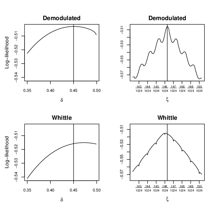
One of the concrete and substantive conclusions of our new estimation procedures is illustrated in Figure 1; this figure illustrates that whereas a standard estimation procedure, based on the Whittle likelihood (see Section 1.3), produces estimates that are, on average, biased even in large samples, our new procedure, based on a carefully constructed likelihood (see Sections 2.2 and 3), produces estimators that exhibit no such bias. Full details of this Figure are given in Section 4.1.
Refer to caption
Figure 1: Simulated Data: Mean standardized likelihoods for the pole (right) and the long memory parameter (left) over 2000 simulations, with sample size of 1024, and the true values of the long memory parameter and the pole taking the values 0.45 and 1/7, respectively. The vertical solid lines indicate the true values of the parameters. The Demodulated likelihood is noted in equation (16) whilst the discrete Whittle likelihood is noted in equation (8). On average, the demodulated likelihood has its mode at the true values, whereas the Whittle likelihood does not. See Section 4.1 for full details.

1.1 Seasonally Persistent Processes

Stationary time-series models with long range dependence describe a wide range of physical phenomena; see for general discussion Andel 1986 and Gray et al. 1989, and also applications in econometrics (Porter-Hudak 1990; Gil-Alana 2002), biology (Beran 1994) and hydrology (Ooms 2001). Dependence in a stationary time series is parameterized via the autocovariance sequence, {γτ}\{\gamma_{\tau}\}. We are concerned with the estimation of parameters that specify γτ\gamma_{\tau} under an assumption of seasonal persistence. Specifically, of particular importance is the seasonality of the data characterized by a frequency, ξ\xi, termed the pole, and an associated degree of dependence, characterized by a persistence (or long memory) parameter δ\delta. Whereas inference for the persistence parameter in the context of poles at frequency zero has been much studied (Beran 1994), the theoretical behaviour of estimators of the persistence parameter remains largely uninvestigated when the underlying seasonality of the process is unknown.

Let {Xt}\{X_{t}\} be a zero-mean, second-order stationary time series with autocovariance (acv) sequence γτ=cov​{Xt,Xt+τ}=E⁡{Xt​Xt+τ}\gamma_{\tau}=\textrm{cov}\left\{X_{t},X_{t+\tau}\right\}={\mathrm{E}}\left\{X_{t}X_{t+\tau}\right\}, and spectral density function (sdf), f⁡(⋅)f(\cdot),

f⁡(λ)=∑τ=−∞∞γτ​e−2​i​π​λ​τ.f\left(\lambda\right)=\sum_{\tau=-\infty}^{\infty}\gamma_{\tau}e^{-2i\pi\lambda\tau}. (1)

The process {Xt}\{X_{t}\} exhibits seasonal or periodic persistence if there exist real numbers H∈(1/2,1)H\in(1/2,1) and ξ∈(0,1/2)\xi\in\left(0,1/2\right), and a bounded function c⁡(γ)c(\gamma) such that

limτ→∞γτc⁡(γ)​|τ|2​H−2=cos⁡(2​π​ξ​τ),\lim_{\tau\rightarrow\infty}\frac{\gamma_{\tau}}{c(\gamma)\left|\tau\right|^{2H-2}}=\cos\left(2\pi\xi\tau\right),

or equivalently if there exist β∈(0,1)\beta\in(0,1) and ξ∈(0,12)\xi\in\left(0,\frac{1}{2}\right) and a bounded function c⁡(λ)c(\lambda) such that

limλ→ξf⁡(λ)​|λ−ξ|βc⁡(λ)=1.\lim_{\lambda\rightarrow\xi}\frac{f(\lambda)\left|\lambda-\xi\right|^{\beta}}{c(\lambda)}=1.

Following convention, we parameterize the persistence parameter via δ=β/2\delta=\beta/2. In line with this definition, a process is considered to be a seasonally persistent process (SPP) if, in a neighbourhood of ξ\xi,

f⁡(λ)=f†​(λ)​|λ−ξ|−β+o​(|λ−ξ|−β),f\left(\lambda\right)=f^{\dagger}\left(\lambda\right)\left|\lambda-\xi\right|^{-\beta}+\text{o}(\left|\lambda-\xi\right|^{-\beta}), (2)

where f†​(λ)≡c⁡(λ)>0f^{\dagger}(\lambda)\equiv c(\lambda)>0, 0<λ<120<\lambda<\frac{1}{2} is bounded above.

Parameters (ξ,δ)(\xi,\delta) determine the dominant long term behaviour of the process; typically, ξ\xi corresponds to the location of an unbounded but integrable singularity in the sdf. In this paper we consider a parametric family of sdfs consistent with (2), that is, the parametric model of Giraitis et al. 2001, where

f⁡(λ)=fG​(λ,ξ,δ,𝜽,σϵ2)=σϵ2​|h⁡(λ,𝜽)|2​(1−2​e−2​i​π​λ​cos⁡(2​π​ξ)+e−4​i​π​λ)−2​δ,f(\lambda)=f_{G}(\lambda;\xi,\delta,\bm{\theta},\sigma_{\epsilon}^{2})=\sigma^{2}_{\epsilon}|h(\lambda\,;\,\bm{\theta})|^{2}(1-2e^{-2i\pi\lambda}\cos(2\pi\xi)+e^{-4i\pi\lambda})^{-2\delta}, (3)

where h⁡(λ,𝜽)h(\lambda\,;\,\bm{\theta}) is bounded above and below at λ=ξ\lambda=\xi, with some linear process assumptions, given for instance in Hannan 1973; for example, h⁡(⋅)h(\cdot) could be the sdf for a stationary and invertible ARMA process, such is the case for GARMA processes, see Gray et al. 1989. We consider behaviour near the pole in such models by defining f†​(λ)f^{\dagger}(\lambda), where

f⁡(λ)=f†​(λ)​|λ−ξ|−2​δ=f†​(λ,ξ,δ,𝜽)​|λ−ξ|−2​δ.\displaystyle f\left(\lambda\right)=f^{\dagger}(\lambda)\left|\lambda-\xi\right|^{-2\delta}=f^{\dagger}(\lambda;\xi,\delta,\bm{\theta})\left|\lambda-\xi\right|^{-2\delta}. (4)

The results in this paper will also be applicable to nearly non-stationary unit root AR processes, when the roots of the AR process approach unity at a suitable rate in the sample size, this quantifying issues with near unit root processes.

1.2 Estimation for Seasonally Persistent Processes

We consider maximum likelihood estimation of ξ\xi and δ\delta, and denote the true values of these parameters by (ξ⋆,δ⋆)(\xi^{\star},\delta^{\star}). Joint estimation of the seasonality and persistence parameters is of importance, as inaccurate estimation of ξ\xi will affect the estimation of δ\delta, and any other parameters of the sdf – δ\delta quantifies the rate of decay of the dependence, and thus determines the long-term behaviour of the series. Note also that, even in cases where ξ\xi is believed to be known (for calendar data, equal to 1/12, or 1/7, or 1/4 say), there may on occasion be finite sample advantage in estimating ξ\xi rather than using its known value, in terms of estimation of the other parameters of the system. For example, if ξ\xi is regarded as a nuisance parameter, then δ\delta may be more efficiently estimated after conditioning on ξ^\widehat{\xi} rather than ξ⋆\xi^{\star}; see, for example, Robins et al. 1994 and Rathouz et al. 2002 for supporting theory. This issue goes beyond the scope of this paper, but gives further indication that estimation of ξ\xi is intrinsically important.

We will examine inference for the parameters of an SPP based on a realization of the process of length NN. Throughout this paper, for convenience and with minimal loss of generality, we will assume NN is even, N=2​MN=2M say. We establish asymptotic results for these estimators (ξ^,δ^)(\widehat{\xi},\widehat{\delta}), and provide practically useful large sample approximations to the distribution of the estimators. In particular, we define a large sample approximation to the log-likelihood of the periodogram evaluated at a full set of frequencies spaced O​(N−1)\text{O}(N^{-1}) apart. At a local scale the variational structure of the log-likelihood in ξ\xi remains appreciable over O​(N−1)\text{O}(N^{-1}) distances; however the magnitude of these variations becomes negligible compared to the total accumulated magnitude of the log-likelihood for increasing sample sizes. We demonstrate that this variation prevents standard likelihood results being valid for the estimator of ξ\xi, although standard asymptotic results can be established for the estimator of the δ\delta, which is in agreement with previous results, see (Hidalgo and Soulier 2004; Giraitis et al. 2001). We discuss in detail the large sample behaviour of N⁡(ξ^−ξ⋆)N(\widehat{\xi}-\xi^{\star}) and establish its approximate large sample distribution, as well as a moderate sample size approximation. Finally we demonstrate that our likelihood-based estimators have good small sample properties on simulated series compared with other, non-likelihood estimators, and consider estimation of the system parameters in a econometric example, using a data set with weekly gasoline sales in the United States, and two meteorological examples, monthly temperature data from a Californian shore-station, and the Southern Oscillation Index data set.

1.3 The Periodogram, Likelihoods and Approximations

We consider a sample from a stationary Gaussian time series, 𝑿=(X0,X1,…,XN−1)⊤\bm{X}=\left(X_{0},X_{1},\dots,X_{N-1}\right)^{\top}, as defined in section 1.1, with covariance matrix 𝒢N=𝒢N​(ξ,δ,𝜽,σϵ2){\mathcal{G}}_{N}={\mathcal{G}}_{N}(\xi,\delta,\bm{\theta},\sigma^{2}_{\epsilon}) with (i,j)th(i,j)^{\textrm{th}} element γ|i−j|\gamma_{\left|i-j\right|}. The exact log likelihood, ℓN\ell_{N}, of the finite time-domain sample is given by

2​ℓN​(ξ,δ,𝜽,σϵ2)=2​log⁡LN​(ξ,δ,𝜽,σϵ2)=−N​log⁡(2​π)−log⁡|𝒢N|−𝑿⊤​𝒢N−1​𝑿.2\ell_{N}\left(\xi,\delta,\bm{\theta},\sigma^{2}_{\epsilon}\right)=2\log L_{N}\left(\xi,\delta,\bm{\theta},\sigma^{2}_{\epsilon}\right)=-N\log\left(2\pi\right)-\log\left|{\mathcal{G}}_{N}\right|-\bm{X}^{\top}{\mathcal{G}}_{N}^{-1}\bm{X}. (5)

This likelihood is often approximated due to the computational complexity associated with the calculation of 𝒢N−1{\mathcal{G}}_{N}^{-1}. The standard approximation approach was introduced by Whittle 1951, and the resulting, much studied, discretized approximate likelihood is commonly known as the discrete Whittle likelihood. The Whittle likelihood gives an approximation to the likelihood of the time domain data in the frequency domain via the Fourier coefficients, under assumptions as specified by Beran 1994. Problems associated with the usage of Whittle’s approximation for non-Gaussian and small sample size Gaussian time series has been discussed by Contreras-Cristan et al. 2006.

The final two terms in equation (5) are approximated using results of Whittle 1951 and Grenander and Szegö 1984. It follows that the Whittle likelihood for (ξ,δ)(\xi,\delta) and 𝜽\bm{\theta} is given by:

ℓN(W)(ξ,δ,𝜽,σϵ2)=−∫−1212I0​(λ)f⁡(λ)dλ,\ell_{N}^{(W)}\left(\xi,\delta,\bm{\theta},\sigma^{2}_{\epsilon}\right)=-\int_{-\frac{1}{2}}^{\frac{1}{2}}\frac{I_{0}\left(\lambda\right)}{f\left(\lambda\right)}\;d\lambda, (6)

where I0​(λ)I_{0}\left(\lambda\right) is the periodogram, defined as the modulus square of the discrete Fourier transform (DFT), Z0​(λ)Z_{0}\left(\lambda\right), of the realized time series.

At the Fourier frequencies φj=j/N{\varphi_{j}}=j/N, j=0,…,Mj=0,\ldots,M, the periodogram, I0I_{0}, is given by, I0​(φj)=|Z0​(φj)|2I_{0}({\varphi_{j}})=|Z_{0}({\varphi_{j}})|^{2} where

Z0(φj)=1N∑t=0N−1Xte−i​2​π​t​φj=A0(φj)−iB0(φj),j=0,…,M,Z_{0}({\varphi_{j}})=\frac{1}{\sqrt{N}}\sum_{t=0}^{N-1}X_{t}e^{-i2\pi t{\varphi_{j}}}=A_{0}({\varphi_{j}})-iB_{0}({\varphi_{j}}),\quad j=0,\ldots,M, (7)

so that

I0(φj)=A02(φj)+B02(φj)=1N[∑t=0N−1Xt2+2∑t=1N−1∑s=0t−1XtXscos{2πj(t−s)/N}].I_{0}({\varphi_{j}})=A_{0}^{2}({\varphi_{j}})+B_{0}^{2}({\varphi_{j}})=\frac{1}{N}\left[\sum_{t=0}^{N-1}X_{t}^{2}+2\sum_{t=1}^{N-1}\sum_{s=0}^{t-1}X_{t}X_{s}\cos\left\{2\pi j(t-s)/N\right\}\right].

For short memory data, the periodogram is an asymptotically unbiased but inconsistent estimator of f⁡(⋅)f(\cdot) that is commonly used as the basis of more sophisticated estimation procedures. The use of (6) for parameter estimation has been discussed in detail by Walker 1964; Walker 1965 and Hannan 1973 under the assumption that the log spectrum integrates to zero. Hosoya 1974 added a second term of log⁡{f⁡(λ)}\log\left\{f(\lambda)\right\} to the integral to deal with more general processes.

For the likelihood in equation (6) to have desirable asymptotic properties, it is assumed that the process is linear, and satisfies certain regularity conditions, thus ensuring good large sample properties of the likelihood based estimators. Note that (6) is an approximation to the log-likelihood of 𝑿\bm{X} based on the periodogram, but that (6) is not a likelihood for the periodogram. The approximation of the likelihood in equation (5) by equation (6), performs well when the process is Gaussian and the covariance of the time series is either rapidly decaying or exactly periodic.

A Riemann approximation to the integral in equation (6) yields the discrete analogue

ℓN(D​W)(ξ,δ,𝜽,,σϵ2)=−2N∑j=0MI0​(φj)f⁡(φj),\ell_{N}^{(DW)}(\xi,\delta,\bm{\theta},,\sigma^{2}_{\epsilon})=-\frac{2}{N}\sum_{j=0}^{M}\frac{I_{0}(\varphi_{j})}{f(\varphi_{j})}, (8)

and we could also adjust this to allow for more general processes:

ℓN(D​W)(ξ,δ,𝜽,,σϵ2)=−2N∑j=0MI0​(φj)f⁡(φj)−2N∑j=0Mlog[f(φj)],\ell_{N}^{(DW)}(\xi,\delta,\bm{\theta},,\sigma^{2}_{\epsilon})=-\frac{2}{N}\sum_{j=0}^{M}\frac{I_{0}(\varphi_{j})}{f(\varphi_{j})}-\frac{2}{N}\sum_{j=0}^{M}\log[f(\varphi_{j})], (9)

following Hosoya’s proposal. By defining the vector 𝑪2​j,2​j+1​(Aj,Bj)⊤,\bm{C}_{2j,2j+1}(A_{j},\;B_{j})^{\top}, where Aj=A0​(φj)A_{j}=A_{0}({\varphi_{j}}) and Bj=B0​(φj)B_{j}=B_{0}({\varphi_{j}}), and 𝚺𝑪\bm{\Sigma}_{\bm{C}} as the exact covariance of 𝑪\bm{C}, we may consider the exact log-likelihood, ℓN(f)\ell_{N}^{(f)} of the DFT of observed and Gaussian data via:

2​ℓN(f)​(ξ,δ,𝜽,σϵ2)=−N​log⁡(2​π)−log⁡|𝚺𝑪|−𝑪⊤​𝚺𝑪−1​𝑪,2\ell_{N}^{(f)}\left(\xi,\delta,\bm{\theta},\sigma^{2}_{\epsilon}\right)=-N\log(2\pi)-\log\left|{\bm{\Sigma}}_{\bm{C}}\right|-\bm{C}^{\top}{\bm{\Sigma}}_{\bm{C}}^{-1}\bm{C}, (10)

in direct analogue with equation (5), acknowledging finite sample effects of the DFT. The difference between this equation and the discrete Whittle likelihood is that it involves the exact covariance matrix, 𝚺𝑪{\bm{\Sigma}}_{\bm{C}}, of the FFT coefficients. Analysis based on the likelihood of the Fourier coefficients (in general) involves the inversion of the large, non-sparse covariance matrix, and is thus equally inefficient as the basis of likelihood procedures as equation (5).

Having specified these various likelihood functions that could be used for inference, some justification must be used to motivate their usage. Equation (10) is a natural choice for analysis of seasonal time series, given the compression of the variables of the seasonal effects. We shall use the compression to approximate the likelihood more carefully, acknowledging large finite sample effects related to the compression explicitly.

1.4 Contributions of the Paper

We introduce an approximation to equation (10), and use this as the basis of a maximum likelihood procedure. We focus on the distribution and other properties of the periodogram, given an underlying SPP with sdf f⁡(⋅)f(\cdot). We focus on Gaussian processes, and do not consider here the non-Gaussian case. However, for other processes, such as those in Brillinger 1975, where asymptotic normality of the DFT holds, our distributional results are still valid.

Specifically, we consider estimation of parameters of spectra with spectral poles away from frequency zero. We consider an adjustment to the standard DFT that simplifies the technical developments of this paper. A simple (but parameter dependent) modification of the choice of grid, conditional on a known spectral pole location, leads to simple approximations to the likelihood of the periodogram at a new set of frequencies spaced at a distance O​(N−1)\text{O}(N^{-1}) apart. In particular

  1. 1.

    We propose a new demodulated Whittle discrete likelihood for seasonal processes (sections 2 & 3). We show that the proposed likelihood approximates the distribution of the discrete Fourier transform for any posited value of the true parameters (see Theorem 1). The key idea is to use a different orthogonal transformation of the data conditional on each fixed value of the location of the pole (specification of a compressed representation). This is a non-standard situation.

  2. 2.

    To establish the properties of the likelihood we calculate the large finite sample distribution of the periodogram at the pole itself (Section 2.3).

  3. 3.

    We bound the covariance of the demodulated periodogram at different frequencies spaced 1/N1/N apart (noted in Section 3), and note its asymptotically negligible contribution to the normalized log-likelihood. Furthermore, the choice of approximation to the likelihood is not everywhere continuous. However, we demonstrate (Section 3) that the discontinuities in the likelihood surface represent a negligible contribution for finite large samples.

  4. 4.

    We prove consistency of the MLEs (see Theorem 2), and determine the large sample first order properties of the score and observed Fisher information (Theorem 3).

  5. 5.

    We determine the asymptotic distribution of the score and observed Fisher information (see Theorem 4) and the asymptotic distribution of the MLEs (see Theorem 5).

  6. 6.

    We give a large finite sample approximation to the distribution of the pole estimator (see Proposition 6).

To derive the appropriate large sample theory, some care is required. It transpires that the score and Fisher information do not exhibit the usual large sample behaviour. Our results are based on a Taylor expansion of the log-likelihood; we adopt the normalization of the observed Fisher information adopted by Sweeting 1980; Sweeting 1992. We thus renormalize the observed Fisher information appropriately with a suitable power of NN. The renormalized score and observed Fisher information converge in law to Gaussian random variables that are asymptotically uncorrelated. The distribution of ξ^\widehat{\xi} converges slowly to the asymptotic distribution, and so alternate finite large sample approximations are also given.

These results establish a new large sample theory for seasonally persistent processes, and utilize the data-dependent transformation of the time-domain data that facilitate the computation of the distribution of different random variables for each posited value of the pole, and appropriate normalisation techniques for the score and Fisher information when the data is modelled as highly compressed in the Fourier domain.

1.5 Connections with Recent Work

In connections with other related work, we distinguish between likelihood-based methods and semi-parametric methods for processes exhibiting seasonal persistence. Giraitis et al. 2001 consider fully parametric models, and constrain the maximization over the location to a grid of frequencies spaced O​(N−1)\text{O}(N^{-1}) apart. Hidalgo and Soulier 2004 consider semi-parametric models, and the theoretical properties of the extended Geweke-Porter-Hudak estimator, basing their analysis on estimating the location of the singularity as the Fourier coefficient of the maximum periodogram value in a given frequency interval; in their simulation study, the true location of the singularity is aligned with the Fourier frequency grid. Hidalgo and Soulier 2004 evaluate the Fourier coefficients at the Fourier frequency grid, and restrict the estimate of the location of the pole to a grid of frequencies spaced O​(N−1)\text{O}(N^{-1}) apart. Hidalgo 2005 used semi-parametric methods to estimate the location of the pole, as well as the long memory parameter. By using a two-step procedure he is able to develop large sample theory for the estimator of the singularity, whereas in contrast we focus on full likelihood methods. More recently, Whitcher 2004 used a wavelet packet analysis approach for estimation of seasonally persistent processes.

In terms of asymptotic properties, our rate of convergence matches that of Giraitis et al. 2001. However, in addition, we obtain the large sample distributional results for the estimator of the pole, which they fail to do, having produced a different estimator. Similarly to Giraitis’ et al., Beran and Gosh 2000 estimate the location of the pole using the coefficient which maximises the periodogram. Our estimator is again different although asymptotically equivalent with the same rate of convergence, and it has a determinable asymptotic, as well as large finite sample approximate, distribution.

Our work also has a connection with, but is different in spirit from, hidden frequency estimation, in which the seasonal structure is modelled as deterministic, corresponding to a single sinusoid. In this case, the Fourier coefficient which maximizes the periodogram converges to the true coefficient with a faster rate than the convergence of the MLE of the pole. Such rates were improved by secondary analysis, and the corresponding analysis using data tapers, see for example Chen et al. 2000; Hannan 1973; Hannan 1986; v. Sachs 1993. Secondary analysis corresponds to partitioning the time series into several groups of data, and using regression to estimate the so-called hidden frequency. Thomson 1990 used multitaper methods to improve the detection of a set of hidden frequencies, and use least squares methods over a given bandwidth. Neither the model we use, nor our proposed inferential method, is equivalent to the above mentioned procedures. Secondary analysis can be considered to ‘zoom in’ on local structure near the pole, and may be philosophically related to our procedure, but we implement full likelihood for a full set of Fourier coefficients. Conditionally for each fixed value for the pole, we calculate the distribution of a different set of random variables, but as each set is a linear and orthogonal transformation of the original data, and with a constant and equal Jacobian, this is appropriate.

Finally, we note that the inferential issues are of importance beyond seasonally persistent processes. The inherent non-regularity arises due to a parameter dependent transformation of the time-domain data. Whenever the process is modelled using a suitable parametric linear transformation of the data that will give decomposition coefficients that are non-negligible only for a few sets of indices, our methods will be applicable with some minor modifications. In a more general setting we would write the variances of a set of basis coefficients as satisfying a power-law decay, and we refer to such processes as second order compressive processes. Power-law decay in a suitable basis is an relatively common phenomenon - see for example the discussion in Donoho 2006; Abramovich et al. 2006; Candès and Tao 2004 - and our developments will carry across to this setting if the compression is stochastic rather than deterministic, once the location and decay parameters have been incorporated in the arbitrary basis. Issues of alignment, and/or shift-variance, akin to results that arise for misspecified location of the pole, are very well-documented in other basis expansions (Coifman and Donoho 1995). Note that the equivalent to the decay parameter discussed by the aforementioned authors will be p=1/(2​δ)p=1/(2\delta). Only for δ>0.25\delta>0.25 are we in their mode of decay, corresponding to extreme regimes of long memory behaviour.

2 Distributional results for the Periodogram

2.1 Large Sample Properties

The large sample properties of the periodogram of seasonally persistent processes were determined in Olhede et al. 2004. We summarize and extend these results below; in particular we compute the statistical properties of the periodogram itself at the pole ξ\xi, as this specific Fourier coefficient will contribute substantively to the subsequent likelihood calculation.

Theorem 1 in Olhede et al. 2004 gives the following result concerning the relative bias at frequency λ\lambda, Bλ,N​(ξ,δ)B_{\lambda,N}(\xi,\delta), of the periodogram for all λ∈(−1/2,1/2),ξ∈(0,1/2)\lambda\in(-1/2,1/2),\xi\in(0,1/2),

Bλ,N​(ξ,δ)={E​{I0​(λ)f⁡(λ)}λ≠ξE​{I0​(ξ)N2​δ​f†​(ξ)}λ=ξB_{\lambda,N}(\xi,\delta)=\left\{\begin{array}[]{ll}{\mathrm{E}}\left\{\dfrac{I_{0}(\lambda)}{f(\lambda)}\right\}&\qquad\lambda\neq\xi\\[12.0pt] {\mathrm{E}}\left\{\dfrac{I_{0}(\xi)}{N^{2\delta}f^{\dagger}(\xi)}\right\}&\qquad\lambda=\xi\end{array}\right.

This notation makes explicit the dependence of the relative bias on ξ\xi and NN. For frequencies φk=k/N,k∈{0,…,M}{\varphi_{k}}=k/N,k\in\left\{0,\ldots,M\right\}, we have, for large NN and a fixed value of ξ\xi, with φk≠ξ{\varphi_{k}}\neq\xi,

Bφk,N​(ξ,δ)=2π​∫−∞∞[sin⁡{u/2−π​cN​(ξ,φk)}u−2​π​cN​(ξ,φk)]2​|2​π​cN​(ξ,φk)u|2​δ​𝑑u+o​(1),B_{{\varphi_{k}},N}(\xi,\delta)=\frac{2}{\pi}\int_{-\infty}^{\infty}\left[\frac{\sin\{u/2-\pi c_{N}(\xi,{\varphi_{k}})\}}{u-2\pi c_{N}(\xi,{\varphi_{k}})}\right]^{2}\left|\frac{2\pi c_{N}(\xi,{\varphi_{k}})}{u}\right|^{2\delta}\;du+\text{o}(1), (11)

where cN​(ξ,φk)=N⁡(φk−ξ)c_{N}(\xi,{\varphi_{k}})=N({\varphi_{k}}-\xi) denotes NN times the distance between the kt​hk^{th} Fourier frequency and the pole at ξ\xi. For the case φk=ξ{\varphi_{k}}=\xi, the large sample value of Bξ,N​(ξ,δ)B_{\xi,N}\left(\xi,\delta\right) is given in Lemma 1 in Section 2.4.

For the second order moment properties, let

Cφk,φl,N​(u,ξ)\displaystyle C_{\varphi_{k},\varphi_{l},N}(u,\xi) =\displaystyle= sin{u/2−πcN(ξ,φk)}sin{u/2−πcN(ξ,φl)}{u−2​π​cN​(ξ,φk)}​{u−2​π​cN​(ξ,φl)}\displaystyle\frac{\sin\{u/2-\pi c_{N}(\xi,{\varphi_{k}})\}\sin\{u/2-\pi c_{N}(\xi,{\varphi_{l}})\}}{\{u-2\pi c_{N}(\xi,{\varphi_{k}})\}\{u-2\pi c_{N}(\xi,{\varphi_{l}})\}}
Vφk,φl,N​(ξ,δ)\displaystyle{V}_{\varphi_{k},\varphi_{l},N}\left(\xi,\delta\right) =\displaystyle= (−1)k+l​2π​∫−∞∞Cφk,φl,N​(u,ξ)​|2​πu|2​δ​|cN​(ξ,φk)​cN​(ξ,φl)|δ​𝑑u+o​(1).\displaystyle\left(-1\right)^{k+l}\frac{2}{\pi}\int_{-\infty}^{\infty}C_{\varphi_{k},\varphi_{l},N}\left(u,\xi\right)\left|\frac{2\pi}{u}\right|^{2\delta}|c_{N}(\xi,{\varphi_{k}})c_{N}(\xi,{\varphi_{l}})|^{\delta}\;du+\text{o}(1).

Then, for A0​(φj),B0​(φj)A_{0}({\varphi_{j}}),B_{0}({\varphi_{j}}) from (7), Olhede et al. 2004 gives

E⁡{A0​(φk)​A0​(φl)}=E⁡{B0​(φk)​B0​(φl)}\displaystyle{\mathrm{E}}\{A_{0}({\varphi_{k}})A_{0}({\varphi_{l}})\}={\mathrm{E}}\{B_{0}({\varphi_{k}})B_{0}({\varphi_{l}})\} =\displaystyle= {Vφk,φl,N​(ξ,δ)/2+o​(1)}​f⁡(φk)​f​(φl)\displaystyle\{V_{\varphi_{k},\varphi_{l},N}(\xi,\delta)/2+\text{o}(1)\}\sqrt{f({\varphi_{k}})f({\varphi_{l}})}
E⁡{A0​(φk)​B0​(φl)}=E⁡{B0​(φk)​A0​(φl)}\displaystyle{\mathrm{E}}\{A_{0}({\varphi_{k}})B_{0}({\varphi_{l}})\}={\mathrm{E}}\{B_{0}({\varphi_{k}})A_{0}({\varphi_{l}})\} =\displaystyle= o​(1)​f⁡(φk)​f​(φl)\displaystyle\text{o}(1)\sqrt{f({\varphi_{k}})f({\varphi_{l}})}
=\displaystyle= o​(N2​δ)ifcN​(ξ,φk),cN​(ξ,φl)=O⁡(1).\displaystyle\text{o}\left(N^{2\delta}\right)\quad{\mathrm{if}}\quad c_{N}(\xi,{\varphi_{k}}),\;c_{N}(\xi,{\varphi_{l}})=O(1).

These results specify the large sample first and second order structure of the periodogram. We now extend these results to the demodulated periodogram described in section 2.2. Note that a direct implication of these results is that the distribution of the periodogram is highly dependent on the distances between the pole ξ\xi and the Fourier frequencies {φk}\{{\varphi_{k}}\}.

2.2 The Demodulated Discrete Fourier Transformation

The Discrete Fourier Transform of {Xt}\{X_{t}\} is not constrained to be evaluated at {φk}\{{\varphi_{k}}\}, but in fact any O​(N−1)\text{O}(N^{-1}) grid could be considered. This fact leads us to consider demodulation, a grid realignment technique, which for any fixed value of ξ\xi produces a new grid aligned with the pole. Demodulation ensures that the large sample behaviour of the demodulated periodogram is similar to that of the periodogram of a standard long memory process (where ξ=0\xi=0). Specifically, the large sample bias is the same but the distribution of the periodogram is χ22\chi^{2}_{2} rather than a sum of unequally weighted χ12\chi^{2}_{1} random variables (see Hurvich and Beltrao 1993; Olhede et al. 2004, p. 621).

The Demodulated Discrete Fourier Transform (DDFT) or offset DFT (Pei and Ding 2004) of a sample of size NN from time series {Xt}\{X_{t}\} with demodulation via a fixed frequency λ\lambda is denoted ZλZ_{\lambda}, and is defined for Fourier frequency φj{\varphi_{j}} by

Zλ(φj)=1N∑t=0N−1Xte−2​i​π​(φj+λ)​t=Aλ(φj)−iBλ(φj),j=0,…,M.Z_{\lambda}({\varphi_{j}})=\frac{1}{\sqrt{N}}\sum_{t=0}^{N-1}X_{t}e^{-2i\pi({\varphi_{j}}+\lambda)t}=A_{\lambda}({\varphi_{j}})-iB_{\lambda}({\varphi_{j}}),\quad j=0,\ldots,M. (12)

The demodulated periodogram at frequency φj{\varphi_{j}} with demodulation via λ\lambda is denoted Iλ​(φj)I_{\lambda}({\varphi_{j}}), and is defined via the ordinary periodogram I0I_{0} by

Iλ​(φj)=I0​(φj+λ)=|Zλ​(φj)|2=Aλ2​(φj)+Bλ2​(φj).I_{\lambda}({\varphi_{j}})=I_{0}({\varphi_{j}}+\lambda)=|Z_{\lambda}({\varphi_{j}})|^{2}=A_{\lambda}^{2}({\varphi_{j}})+B_{\lambda}^{2}({\varphi_{j}}).

Hence Iλ​(φj)I_{\lambda}({\varphi_{j}}) is simply the periodogram evaluated at frequency φj+λ,{\varphi_{j}}+\lambda, or I0​(φj+λ).I_{0}({\varphi_{j}}+\lambda). We will consider evaluating this expression at arbitrary frequency φ\varphi. We define Cλ;2​j,2​j+1=(Aλ,j,Bλ,j)⊤={Aλ​(φj),Bλ​(φj)}⊤,C_{\lambda;2j,2j+1}=(A_{\lambda,j},B_{\lambda,j})^{\top}=\{A_{\lambda}({\varphi_{j}}),\;B_{\lambda}({\varphi_{j}})\}^{\top}, in analogue to 𝑪\bm{C} in equation (10). For Gaussian data 𝑿\bm{X} we then find:

𝑪λ=(Aλ,0,Bλ,0,…​Aλ,M,Bλ,M)T​=𝔏​𝒩​(𝟎,𝚺𝑪λ)\bm{C}_{\lambda}=\left(A_{\lambda,0},B_{\lambda,0},\dots A_{\lambda,M},B_{\lambda,M}\right)^{T}\overset{\mathfrak{L}}{=}\mathcal{N}\left(\bm{0},\bm{\Sigma}_{\bm{C}_{\lambda}}\right) (13)

Note that due to the demodulation, Bλ,0≠0B_{\lambda,0}\neq 0 in general, unlike the imaginary component of the DFT at frequency zero. To efficiently formulate the likelihood, we need to explicitly consider the computation of 𝚺𝑪λ\bm{\Sigma}_{\bm{C}_{\lambda}}, the covariance of the DDFT coefficients.

2.3 Extending the Olhede et al. 2004 result

The results in Olhede et al. 2004 do not cover the case of demodulation, and to enable calculation of the new likelihood, further results are required. For example Bξ,N​(ξ,δ)B_{\xi,N}(\xi,\delta) needs to be explicitly determined. To minimize the bias in the demodulated periodogram, and simplify the covariance structure, we shift the Fourier grid so that the closest Fourier frequency to the pole in the original grid coincides exactly with the pole in the demodulated version. For a pole at ξ\xi, we denote by j0,N​(ξ)=[N​ξ],j_{0,N}(\xi)=[N\xi], where [x][x] indicates the nearest integer to x.x. We furthermore let cN​(ξ,φj0,N​(ξ))=j0,N​(ξ)−N​ξc_{N}(\xi,\varphi_{j_{0,N}(\xi)})=j_{0,N}(\xi)-N\xi and specify λ=λD,N​(ξ)\lambda=\lambda_{D,N}(\xi) in (12) as λD,N(ξ)=−cN(ξ,φj0,N​(ξ))/N\lambda_{D,N}(\xi)=-c_{N}(\xi,\varphi_{j_{0,N}(\xi)})/N. The approach introduces a new grid of frequencies, namely

λk≡λk⁡(j),N​(ξ)=φj+cN​(ξ,φj0,N​(ξ))N=ξ+j−j0,N​(ξ)N=ξ+k⁡(j)N.\lambda_{k}\equiv\lambda_{k(j),N}(\xi)=\varphi_{j}+\frac{c_{N}(\xi,\varphi_{j_{0,N}(\xi)})}{N}=\xi+\frac{j-j_{0,N}(\xi)}{N}=\xi+\frac{k(j)}{N}. (14)

We exclude Fourier frequencies 00 and 1/21/2, and taking j=1,…,M−1j=1,\dots,M-1 we have k=k⁡(j)=j−j0,N​(ξ)≡J1,…,J2≡−j0,N​(ξ),…,M−j0,N​(ξ)k=k(j)=j-j_{0,N}(\xi)\equiv J_{1},\dots,J_{2}\equiv-j_{0,N}(\xi),\dots,M-j_{0,N}(\xi). For example, if N=16N=16 and ξ=0.15\xi=0.15, then λD,16​(0.15)=0.025\lambda_{D,16}(0.15)=0.025, [N​ξ]=2[N\xi]=2, J1=−1J_{1}=-1 and J2=5J_{2}=5. Note that for k⁡(j2)>k⁡(j1)≠0k(j_{2})>k(j_{1})\neq 0, then

Vλk⁡(j1),λk⁡(j2),N​(ξ,δ)=Vφj1,φj2,N​{j0,N​(ξ)N,δ},V_{\lambda_{k(j_{1})},\lambda_{k(j_{2})},N}(\xi,\delta)=V_{\varphi_{j_{1}},\varphi_{j_{2}},N}\left\{\frac{j_{0,N}(\xi)}{N},\delta\right\},

so that the covariance properties of the DDFT can be easily determined.

Under this demodulation, the DDFT yields the original periodogram I0I_{0} evaluated at frequencies λk≡λk⁡(j)=ξ+(j−j0,N​(ξ))/N,\lambda_{k}\equiv\lambda_{k(j)}=\xi+(j-j_{0,N}(\xi))/N, and takes the form

ZλD(φj)=Z0(λk⁡(j))=1N∑t=0N−1Xte−2​i​π​λk​t,k=J1,…,J2,Z_{\lambda_{D}}\left({\varphi_{j}}\right)=Z_{0}\left(\lambda_{k(j)}\right)=\frac{1}{\sqrt{N}}\sum_{t=0}^{N-1}X_{t}e^{-2i\pi\lambda_{k}t},\quad k=J_{1},\ldots,J_{2}, (15)

so that, for k=J1,…,J2k=J_{1},\ldots,J_{2}, IλD​(φj)=I0​(λk)=I0​(ξ+k/N).I_{\lambda_{D}}({\varphi_{j}})=I_{0}(\lambda_{k})=I_{0}(\xi+k/N). The DDFT can be computed efficiently by applying the DFT to the new series {Yt},\{Y_{t}\}, defined for t=0,…,N−1,t=0,\ldots,N-1, by Yt=Xt​exp⁡{−2​π​i​λD​t}Y_{t}=X_{t}\exp\left\{-2\pi i\lambda_{D}t\right\}. Demodulation both simplifies the mathematical calculations considerably, and improves estimation of the persistence parameter δ.\delta. Naturally the operation is very straightforward to implement. The parameter dependent choice of {λk}\{\lambda_{k}\} will need careful analysis when deriving properties of the parameter estimators.

2.4 Expectation of the Periodogram at the Pole

The result in (11) gives the relative bias of periodogram. The expectation of the periodogram is given in the following Lemma.

Lemma 1

The expected value of the periodogram evaluated at the pole ξ\xi, after demodulation by ξ\xi, is

E​{I0​(ξ)}\displaystyle E\left\{I_{0}(\xi)\right\} =\displaystyle= (2πN)2​δ{−2f†(ξ)Γ(−1−2δ)}cos{π(1/2+δ)}π−1+o(1)\displaystyle(2\pi N)^{2\delta}\{-2f^{\dagger}(\xi)\Gamma(-1-2\delta)\}\cos\{\pi(1/2+\delta)\}\pi^{-1}+\text{o}(1)
=d​e​f\displaystyle\overset{def}{=} N2​δ​f†​(ξ)​𝑩ξ​(ξ,δ)+o​(1)=O​(N2​δ).\displaystyle N^{2\delta}f^{\dagger}(\xi)\mbox{\boldmath$B$}_{\xi}(\xi,\delta)+\text{o}(1)=\text{O}(N^{2\delta}).

Proof: See Appendix A.1.  

3 Asymptotic Properties of the Likelihood and Estimators

In this section we utilize demodulation, and the large sample approximations described above, to present three theorems that characterize the asymptotic behaviour of the likelihood, the corresponding MLEs for (ξ,δ)(\xi,\delta) and the associated Fisher information to obtain their large sample properties. Specifically, we establish NN-consistency for the estimator of the location of the pole, thus matching the result of Giraitis et al. 2001.

3.1 Large-sample Likelihood Approximation

For a periodogram demodulated to align the Fourier grid with pole ξ\xi, we have the following asymptotic result.

Theorem 2

Approximating the Likelihood Function.
For a Gaussian series from a periodic long memory model as described by (3), where f†​(⋅)f^{\dagger}(\cdot) is twice partially differentiable with respect to (ξ,δ)(\xi,\delta), the log-likelihood of the discrete Fourier transform can be approximated by

ℓ⁡(ξ,δ,𝜽,σϵ2)\displaystyle\ell\left(\xi,\delta,\bm{\theta},\sigma^{2}_{\epsilon}\right) =\displaystyle= ∑j=J1J2{log⁡ηj−ηj​I0​(ξ+j/N)}\displaystyle\sum_{j=J_{1}}^{J_{2}}\left\{\log\eta_{j}-\eta_{j}I_{0}(\xi+j/N)\right\} (16)

accurate to o⁡(N)o(N), where

ηj=|j|2δΥ{j≠0}𝑩ξ(ξ,δ)Υ{j=0}N2​δfj†\eta_{j}=\frac{|j|^{2\delta\Upsilon{\{j\neq 0\}}}}{\mbox{\boldmath$B$}_{\xi}(\xi,\delta)^{\Upsilon{\{j=0\}}}N^{2\delta}f_{j}^{\dagger}} (17)

for 0<δ<0.50<\delta<0.5, where Υ​{A}\Upsilon\{A\} is the indicator function for event AA,

fj†≡f†​(λj)=f†​(ξ+j/N)f^{\dagger}_{j}\equiv f^{\dagger}(\lambda_{j})=f^{\dagger}(\xi+j/N)

and 𝐁ξ​(ξ,δ)\mbox{\boldmath$B$}_{\xi}(\xi,\delta) is the asymptotic relative bias given by Lemma 1.

Proof: See the Appendices A.2-A.4.  

Note I : The approximation to the likelihood is equivalent to that of independent exponential random variables with rate parameters ηj\eta_{j} that depend on jj and δ\delta but not on ξ\xi. In equation (17), the function 𝑩ξ​(ξ,δ)\mbox{\boldmath$B$}_{\xi}(\xi,\delta) appropriately scales the periodogram contribution from the Fourier frequency aligned with ξ\xi. 𝑩ξ​(ξ,δ)\mbox{\boldmath$B$}_{\xi}(\xi,\delta) is monotonically increasing in δ\delta, with limx→0𝐁ξ​(ξ,x)=1\lim_{x\rightarrow 0}{\mathbf{B}}_{\xi}(\xi,x)=1, and 𝑩ξ​(ξ,δ)\mbox{\boldmath$B$}_{\xi}(\xi,\delta) is bounded away from zero. As the function is monotonic the derivatives of 𝑩ξ​(ξ,δ)\mbox{\boldmath$B$}_{\xi}(\xi,\delta) are also bounded away from zero. If f†​(⋅)f^{\dagger}(\cdot) is also bounded away from zero, then the log likelihood is bounded in ξ\xi and δ\delta. Thus it is possible to find efficiently the MLEs of ξ\xi and δ\delta numerically.

Note II : This likelihood is not differentiable with respect to ξ\xi at all values of ξ\xi; although I˙0​(ξ+j/N)\dot{I}_{0}(\xi+j/N) is available in simple form, the dependence of J1=−j0,N​(ξ)J_{1}=-j_{0,N}(\xi) and J2=M−j0,N​(ξ)J_{2}=M-j_{0,N}(\xi) on ξ\xi renders the overall function discontinuous. However, the discontinuities are O​(1)\text{O}(1) in magnitude, and the log likelihood is uniformly at least O​(N)\text{O}(N), so in fact the discontinuities are negligible, but motivate us to look, in standard fashion, at the NN-standardized likelihood function ℓ⁡(ξ,δ,𝜽,σϵ2)/N\ell(\xi,\delta,\bm{\theta},\sigma^{2}_{\epsilon})/N. See Appendix A.4 for further details.

Note III : The formulation in Theorem 2 summarizes the data in the frequency domain via the demodulated periodogram for a given ξ\xi. We avoid the introduction of the substantial bias and covariance terms found in Olhede et al. 2004, as the demodulated periodogram is perfectly aligned with this singularity. When other demodulations are chosen the likelihood cannot be approximated in such a fashion. Even for frequencies of sufficient distance from any irregular behaviour, the results of Olhede et al. 2004 cannot be applied directly, and to find the approximate Whittle likelihood we additionally need to make assumptions about the spectral density function, and its smoothness (see Dzhamparidze and Yaglom 1983 and Taniguchi and Kakizawa 2000).

Note IV : The result differs with that of Hurvich and Beltrao 1993 in a number of ways. The ordinates subscripted jj and −j-j in the DFT are no longer complex conjugates, and the likelihood at evaluated at λj\lambda_{j} is now approximately χ22\chi_{2}^{2} (rather than a mixture of two different χ2\chi^{2} terms) even for those coefficients closest to the pole. Strictly, the definition for ηj\eta_{j} in equation (17) has an additional term Vλj,λk,N​(ξ,δ)V_{\lambda_{j},\lambda_{k},N}(\xi,\delta) for j,k∈ℤj,k\in\mathbb{Z}, but these terms can be bounded appropriately, and thus contribute in a negligible fashion. The bias at the pole reported in Hurvich and Beltrao 1993 is (identically) present in our formulation, but is o​(N)\text{o}(N), and is thus subsumed into the final term – see Hurvich et al. 1998 for relevant supporting arguments.

3.2 Existence and Consistency of the ML estimators

We now use the results of the previous section to construct likelihood-based estimators of ξ\xi and δ\delta and establish their properties. The following theorem establishes the existence and consistency of the ML estimators derived from the likelihood in Theorem 2.

Theorem 3

Existence and Consistency
For the likelihood of Theorem 2, the ML estimators of ξ\xi and δ\delta, ξ^\widehat{\xi} and δ^\widehat{\delta}, exist and are consistent, with convergence rates NN and N1/2N^{1/2} respectively.

Proof: See Appendix A.5.  

The NN-consistency of ξ^\widehat{\xi} matches the convergence rate of Giraitis et al. 2001. It is unusual to find superconsistent estimators in likelihood based procedures. An intuitive understanding of the rate can be found in the time domain. As we collect N​ξ⋆N\xi^{\star} full periods of the data the periodicity of the data is determined to an accuracy of O​(N−1)\text{O}(N^{-1}). The reason why this rate is achieved is that the log-likelihood is varying O​(N3/2)\text{O}(N^{3/2}) (see proposition 14) over distances in ξ\xi of O​(N−1)\text{O}(N^{-1}) near the value ξ=ξ⋆.\xi=\xi^{\star}. However, the convergence rate is different to that of Chen et al. 2000. The latter model the seasonality as a deterministic seasonal component embedded in stationary noise. In Chen et al. a regression model is employed to estimate the amplitude and locations of the seasonality, and a rate of N−3/2N^{-3/2} rather than N−1N^{-1} is achieved. We employ a different model and hence do not expect the same convergence rates as is achieved by Chen et al..

3.3 Properties of The Fisher Information Matrix

Theorem 4

The Fisher Information.
For a series from a periodic long memory model as described by (3), for large NN, the components of the Fisher information

ℱN=(ℱξ,ξ(N)ℱξ,δ(N)ℱξ,δ(N)ℱδ,δ(N))\bm{{\cal{F}}}_{N}=\left(\begin{array}[]{cc}{{\cal{F}}}^{(N)}_{\xi,\xi}&{{\cal{F}}}^{(N)}_{\xi,\delta}\\ {{\cal{F}}}^{(N)}_{\xi,\delta}&{{\cal{F}}}^{(N)}_{\delta,\delta}\end{array}\right)

are given by

ℱδ,δ(N)=ℱδ,δ​N+o​(N),ℱξ,δ(N)=ℱξ,δ(1)​N+o⁡{log⁡(N)},ℱξ,ξ(N)=ℱξ,ξ​N2+o​(N2),\displaystyle{{\cal{F}}}^{(N)}_{\delta,\delta}={{\cal{F}}}_{\delta,\delta}N+\text{o}(N),~~~~~{{\cal{F}}}^{(N)}_{\xi,\delta}={{\cal{F}}}_{\xi,\delta}^{(1)}N+o\{\log(N)\},~~~~~{{\cal{F}}}^{(N)}_{\xi,\xi}={{\cal{F}}}_{\xi,\xi}N^{2}+\text{o}(N^{2}),

where ℱδ,δ{{\cal{F}}}_{\delta,\delta}, ℱξ,δ(1){{\cal{F}}}_{\xi,\delta}^{(1)} and ℱξ,ξ{{\cal{F}}}_{\xi,\xi} are constants independent of NN but are functions of the true values of ξ\xi and δ\delta.

Proof: See Appendices A.6 and A.7.  

For a full analysis in a regular ML setting, the second order properties of the MLEs can in a general setting be deduced from the above quantities. Large sample properties, specifically consistency and asymptotic variance, may be considered via a Taylor expansion of the log-likelihood, see for example Cheng and Taylor 1995. However, we note that we are not in a standard setting; even if we may expand the log-likelihood near the true value of the parameter, because of the non-standard behaviour of the derivatives of the log-likelihood, the observed Fisher information does not converge to a diagonal matrix with constant entries, but rather the (appropriately standardized) observed Fisher information for ξ\xi converges to a random variable with order one variance. We will discuss the interpretation of the Fisher information in this context, in the appendix. For the derivatives involving the location of the pole, extra terms of magnitude NN are introduced and thus the variance of the observed Fisher information in ξ\xi is O​(N5).\text{O}(N^{5}). The magnitude of the variance of the observed Fisher information in ξ\xi implies that a standardization of the random variable must be employed that results in a negligible expectation of the restandardized random variable. We also therefore discuss the large sample theory of the observed Fisher information.

3.4 The Asymptotic Properties of the MLEs

We now consider the use of the Fisher information to determine the asymptotic variance. Consider a Taylor expansion of the score near the true value 𝝍⋆\bm{\psi}^{\star} of the parameters 𝝍=(ξ,δ)\bm{\psi}=(\xi,\delta) evaluated at the MLE 𝝍^\widehat{\bm{\psi}}. We denote the observed Fisher information by 𝑭N​(𝝍)\bm{{{F}}}_{N}\left(\bm{\psi}\right), and let 𝝍′{\bm{\psi}^{\prime}} lie between 𝝍\bm{\psi} and 𝝍⋆\bm{\psi}^{\star}. We denote by ℓ˙​(𝝍)\dot{\ell}(\bm{\psi}) the score in 𝝍\bm{\psi}, noting that the score is well defined if the log-likelihood is evaluated ignoring the ξ\xi dependence of J1J_{1} and J2J_{2}, see section A-4:

ℓ˙​(𝝍)=(ℓξ​(𝝍)ℓδ​(𝝍)).\dot{\ell}(\bm{\psi})=\left(\begin{array}[]{c}\ell_{\xi}\left(\bm{\psi}\right)\\ \ell_{\delta}\left(\bm{\psi}\right)\end{array}\right). (18)

Then using a first-order expansion of the log likelihood in the usual way for NN sufficiently large, we have the (vector) score function:

ℓ˙(𝝍^)=ℓ˙(𝝍⋆)−𝑭N(𝝍′)(𝝍^−𝝍⋆)⟺𝑭N(𝝍′)(𝝍^−𝝍⋆)=ℓ˙(𝝍⋆)−ℓ˙(𝝍^).\dot{\ell}(\widehat{\bm{\psi}})=\dot{\ell}(\bm{\psi}^{\star})-\bm{{{F}}}_{N}({\bm{\psi}^{\prime}})(\widehat{\bm{\psi}}-\bm{\psi}^{\star})\qquad\Longleftrightarrow\qquad\bm{{{F}}}_{N}({\bm{\psi}^{\prime}})(\widehat{\bm{\psi}}-\bm{\psi}^{\star})=\dot{\ell}(\bm{\psi}^{\star})-\dot{\ell}(\widehat{\bm{\psi}}).

Thus the difference between 𝝍^\widehat{\bm{\psi}} and 𝝍⋆\bm{\psi}^{\star}, when appropriately scaled by the random matrix 𝑭N​(𝝍′)\bm{{{F}}}_{N}({\bm{\psi}^{\prime}}) corresponds to the value of the score at 𝝍⋆\bm{\psi}^{\star} in the usual fashion. The statistical properties of 𝑭N​(𝝍′)\bm{{{F}}}_{N}({\bm{\psi}^{\prime}}) are not straightforward in this non-regular problem, and require further investigation. Following Sweeting 1992, we define a suitable standardization matrix 𝑩N\bm{B}_{N} and the standardized observed Fisher information by

𝑩N=(N5/200N​ℱδ,δ)𝑾N=𝑩N−1/2𝑭N𝑩N−1/2,\bm{B}_{N}=\left(\begin{array}[]{cc}N^{5/2}&0\\ 0&N{{\cal{F}}}_{\delta,\delta}\end{array}\right)\qquad\bm{{{W}}}_{N}=\bm{B}_{N}^{-1/2}\bm{{{F}}}_{N}\bm{B}_{N}^{-1/2}, (19)

as the large sample properties of 𝑾N\bm{{{W}}}_{N} are tractable, and their determination is an important step to finding the large sample properties of the MLE. Specifically, we let

𝑩N−1/2𝑭N(𝝍′)𝑩N−1/2𝑩N1/2(𝝍^−𝝍⋆)=𝑩N−1/2{ℓ˙(𝝍⋆)−ℓ˙(𝝍^)},\bm{B}_{N}^{-1/2}\bm{{{F}}}_{N}({\bm{\psi}^{\prime}}){\bm{B}}_{N}^{-1/2}\bm{B}_{N}^{1/2}(\widehat{\bm{\psi}}-\bm{\psi}^{\star})=\bm{B}_{N}^{-1/2}\{\dot{\ell}(\bm{\psi}^{\star})-\dot{\ell}(\widehat{\bm{\psi}})\},

so that

𝑾N(𝝍′)𝑩N1/2(𝝍^−𝝍⋆)=𝑩N−1/2ℓ˙(𝝍⋆)=𝒌N(𝝍⋆).\bm{{{W}}}_{N}({\bm{\psi}^{\prime}}){\bm{B}}_{N}^{1/2}(\widehat{\bm{\psi}}-\bm{\psi}^{\star})={\bm{B}}_{N}^{-1/2}\dot{\ell}(\bm{\psi}^{\star})=\bm{k}_{N}(\bm{\psi}^{\star}).

The latter expression defines the standardized score 𝒌N​(⋅).\bm{k}_{N}(\cdot). See the Appendix for a full discussion of these quantities. Note that 𝑩N\bm{B}_{N} is the large NN approximation to the Fisher information matrix for δ\delta and corresponds to an appropriate order normalisation for ξ,\xi, thus 𝑾N​(𝝍)\bm{{{W}}}_{N}\left(\bm{\psi}\right) is the observed Fisher information renormalized by 𝑩N{\bm{B}}_{N}.

We note that for NN large enough, the expected value of 𝑾N​(𝝍⋆)\bm{{{W}}}_{N}(\bm{\psi}^{\star}) is the identity matrix for the δ\delta entry, but the expectation of the first entry of 𝑾N​(𝝍⋆)\bm{{{W}}}_{N}(\bm{\psi}^{\star}) is o​(1)\text{o}(1) whilst the variance of the first entry is O​(1).\text{O}(1). In a standard setting the expectation is O​(1)\text{O}(1) and the variance o​(1)\text{o}(1).

Theorem 5

Distribution of the Score and Observed Fisher Information.
For the likelihood of Theorem 2 the standardized score 𝐤N​(𝛙⋆)\bm{k}_{N}(\bm{\psi}^{\star}) and the standardized Observed Fisher information matrix 𝐖N​(𝛙⋆)\bm{{{W}}}_{N}(\bm{\psi}^{\star}) asymptotically have the following properties:

𝒌N​(𝝍⋆)​⟶ℒ​𝒌,𝑾N​(𝝍⋆)​⟶ℒ​𝑾,\bm{k}_{N}(\bm{\psi}^{\star})\overset{\cal{L}}{\longrightarrow}\bm{k},\quad\bm{{{W}}}_{N}(\bm{\psi}^{\star})\overset{\cal{L}}{\longrightarrow}\bm{W}, (20)

where the entries of 𝐤=(k1,k2)⊤\bm{k}=(k_{1},k_{2})^{\top} and 𝐖\bm{W} are uncorrelated and

W11∼𝒩⁡(0,8​π4/15),W12=0,W22=1k1∼𝒩⁡(0,π2/3),k2∼𝒩⁡(0,1).\begin{array}[]{lcccccccccr}W_{11}&\sim&\mathcal{N}\left(0,8\pi^{4}/15\right),&&W_{12}&=&0,&&W_{22}&=&1\\ k_{1}&\sim&\mathcal{N}\left(0,\pi^{2}/3\right),&&k_{2}&\sim&\mathcal{N}\left(0,1\right).&&&&\end{array} (21)

Proof: An outline of the proof given in the Appendix, see Proposition 12, Section A.8.3 and Proposition 15.  

Theorem 6

Distribution of the MLE.
For the likelihood of Theorem 2, the ML estimators of ξ\xi and δ\delta, ξ^\widehat{\xi} and δ^\widehat{\delta} have distributions that for large sample approximately take the form:

N⁡(ξ^−ξ⋆)={N5/2−ℓξ,ξ​(𝝍′)}​{ℓξ​(𝝍⋆)N3/2}​⟶ℒ​52​π​2​C,N(\widehat{\xi}-\xi^{\star})=\left\{\frac{N^{5/2}}{-\ell_{\xi,\xi}({\bm{\psi}^{\prime}})}\right\}\left\{\dfrac{\ell_{\xi}(\bm{\psi}^{\star})}{N^{3/2}}\right\}\>\overset{\cal{L}}{\longrightarrow}\;\frac{\sqrt{5}}{2\pi\sqrt{2}}C,

where CC is distributed according to the standard Cauchy distribution, and

N​(δ^−δ⋆)∼𝒜​𝒩​(0,N​{ℱδ,δ(N)}−1).\sqrt{N}(\widehat{\delta}-\delta^{\star})\sim\mathcal{AN}\left(0,N\left\{{{\cal{F}}}^{(N)}_{\delta,\delta}\right\}^{-1}\right). (22)

An estimator of the asymptotic variance is formed via ℱ^(N)δ,δ=ℱδ,δ(N)​(ξ^,δ^){{\widehat{\cal{F}}}^{(N)}}_{\delta,\delta}={{\cal{F}}}^{(N)}_{\delta,\delta}(\widehat{\xi},\widehat{\delta}). The forms of ℱδ,δ(N)​(ξ,δ){{\cal{F}}}^{(N)}_{\delta,\delta}(\xi,\delta) and ℱδ,δ​(ξ,δ){{\cal{F}}}_{\delta,\delta}(\xi,\delta) are given in the Appendix.

Proof: An outline proof is given in the Appendix, see Proposition 15 and section A.8.1.  

Note : Giraitis et al. 2001 do not find the limiting distribution of their estimator, ξ^G\hat{\xi}_{G}, of ξ\xi. They note that this is an artefact of the maximization over the specified grid. This constraint is not enforced in our approach. Note that E​(|ξ^−ξ^G|)=O⁡(N−1)\mbox{E}(|\widehat{\xi}-\widehat{\xi}_{G}|)=O\left(N^{-1}\right) but that N​|ξ^−ξ^G|N|\widehat{\xi}-\widehat{\xi}_{G}| is not constrained to be zero or even to have a tractable distribution, this result is demonstrated empirically in the simulations. The convergence to the Cauchy for extreme values of δ\delta is quite slow, we provide, in the Appendix, a second approximation to the distribution of the renormalized estimator of the pole, via more carefully approximating the dominant contributions to the mean and variance of the numerator and denominator that define the random variable the estimator follows.

To compare the two large sample and asymptotic forms of the distributions, we refer to Figure 2 (a) and (b). As δ\delta increases in magnitude it takes longer for the large sample approximation to be close the asymptotic distribution, as is obvious from these plots. For a list of critical values of the distribution see Table 10.

The likelihood of the data changes in magnitude dramatically depending on the value of ξ\xi and its alignment with the grid of frequencies at which the periodogram is evaluated, determination of the best value of ξ\xi is pivotal for characterizing the system, and must be the first stage of any analysis. For completeness we now discuss the estimation of the additional parameters, i.e. 𝜽\bm{\theta} and σϵ2\sigma^{2}_{\epsilon}.

3.5 White Noise Variance and Nuisance Parameters

We now consider the estimation of the white noise component and regular spectral component. We model the sdf parametrically by

f⁡(λ)\displaystyle f(\lambda) =σϵ2​|h⁡(λ,𝜽)|2|2​cos⁡(2​π​λ)−2​cos⁡(2​π​ξ)|2​δ,f†​(λ)=|h⁡(λ,𝜽)|2​σϵ2​|λ−ξ|2​δ|2​cos⁡(2​π​λ)−2​cos⁡(2​π​ξ)|2​δ.\displaystyle=\frac{\sigma^{2}_{\epsilon}\left|h(\lambda;\bm{\theta})\right|^{2}}{\left|2\cos\left(2\pi\lambda\right)-2\cos\left(2\pi\xi\right)\right|^{2\delta}},\quad f^{\dagger}(\lambda)=\frac{\left|h(\lambda;\bm{\theta})\right|^{2}\sigma^{2}_{\epsilon}\left|\lambda-\xi\right|^{2\delta}}{\left|2\cos\left(2\pi\lambda\right)-2\cos\left(2\pi\xi\right)\right|^{2\delta}}. (23)

Differentiating ℓ⁡(ξ,δ,𝜽,σϵ2)\ell(\xi,\delta,\bm{\theta},\sigma^{2}_{\epsilon}) from equation (16) with respect to σϵ2\sigma^{2}_{\epsilon} we obtain that:

∂ℓ⁡(ξ,δ,𝜽,σϵ2)∂σϵ2\displaystyle\frac{\partial\ell(\xi,\delta,\bm{\theta},\sigma^{2}_{\epsilon})}{\partial\sigma^{2}_{\epsilon}} =∑j=J1J2{−1σϵ2+ηj​I0​(ξ+j/N)σϵ2}\displaystyle=\sum_{j=J_{1}}^{J_{2}}\left\{-\frac{1}{\sigma^{2}_{\epsilon}}+\frac{\eta_{j}I_{0}\left(\xi+j/N\right)}{\sigma^{2}_{\epsilon}}\right\}
σ^ϵ2/σϵ2\displaystyle\widehat{\sigma}^{2}_{\epsilon}/\sigma^{2}_{\epsilon} =1−J1+J2+1​∑j=J1J2η^j​I0​(ξ+j/N)\displaystyle=\frac{1}{-J_{1}+J_{2}+1}\sum_{j=J_{1}}^{J_{2}}\widehat{\eta}_{j}I_{0}\left(\xi+j/N\right)
η^j\displaystyle\widehat{\eta}_{j} =|j|2​δ^N2​δ^​|2​cos⁡(2​π​λ)−2​cos⁡(2​π​ξ)|2​δ^σϵ2​|h⁡(λ,𝜽^)|2​|λ−ξ|2​δ^.\displaystyle=\frac{\left|j\right|^{2\widehat{\delta}}}{N^{2\widehat{\delta}}}\frac{\left|2\cos\left(2\pi\lambda\right)-2\cos\left(2\pi\xi\right)\right|^{2\widehat{\delta}}}{\sigma^{2}_{\epsilon}|h(\lambda;\widehat{\bm{\theta}})|^{2}|\lambda-\xi|^{2\widehat{\delta}}}. (24)

Thus it follows that (Taylor expanding the other MLEs and using their rates of convergence):

σ^ϵ2/σϵ2\displaystyle\widehat{\sigma}^{2}_{\epsilon}/\sigma^{2}_{\epsilon} =ℒ​12​(−J1+J2+1)​χ2​(−J1+J2+1)2+o​(1),\displaystyle\overset{\mathcal{L}}{=}\frac{1}{2(-J_{1}+J_{2}+1)}\chi^{2}_{2(-J_{1}+J_{2}+1)}+\text{o}(1), (25)

for J1,J_{1}, J2J_{2} sufficiently large. This follows as the estimators of the other parameters of the sdf are nearly unbiased for sufficiently large values of NN. We note that the covariance of σ^ϵ2\widehat{\sigma}^{2}_{\epsilon} with δ^\widehat{\delta} and ξ^\widehat{\xi} can be treated analogously to the results deriving the covariance of ξ^\widehat{\xi} and δ\delta or using standard results for δ\delta and/or 𝜽\bm{\theta} and σ^ϵ2\widehat{\sigma}^{2}_{\epsilon}. Denoting by

h^​(λ)=h⁡(λ,𝜽^)h˙i​(λ,𝜽)=∂|h⁡(λ,𝜽)|2∂θiandh¨i​k​(λ,𝜽)=∂2|h⁡(λ,𝜽)|2∂θi​∂θk,\widehat{h}(\lambda)=h(\lambda;\widehat{\bm{\theta}})\qquad\dot{h}_{i}(\lambda;\bm{\theta})=\frac{\partial\left|h(\lambda;\bm{\theta})\right|^{2}}{\partial\theta_{i}}\qquad{\mathrm{and}}\qquad\ddot{h}_{ik}(\lambda;\bm{\theta})=\frac{\partial^{2}\left|h(\lambda;\bm{\theta})\right|^{2}}{\partial\theta_{i}\partial\theta_{k}},

we determine that

∂ℓ⁡(ξ,δ,𝜽,σϵ2)∂θi\displaystyle\frac{\partial\ell(\xi,\delta,\bm{\theta},\sigma^{2}_{\epsilon})}{\partial\theta_{i}} =−∑j=J1J2h˙i​(λj,𝜽)|h^​(λj)|2{1−ηjI0(λj)}=O(N),\displaystyle=-\sum_{j=J_{1}}^{J_{2}}\frac{\dot{h}_{i}(\lambda_{j};\bm{\theta})}{|\widehat{h}(\lambda_{j})|^{2}}\left\{1-\eta_{j}I_{0}\left(\lambda_{j}\right)\right\}=\text{O}(N),

and

∂2ℓ⁡(ξ,δ,𝜽,σϵ2)∂θi​∂θk\displaystyle\frac{\partial^{2}\ell(\xi,\delta,\bm{\theta},\sigma^{2}_{\epsilon})}{\partial\theta_{i}\partial\theta_{k}} =∑j=J1J2[−h¨i​k​(λj,𝜽)|h^​(λj)|2​{1−ηj​I0​(λj)}+h˙i​(λj,𝜽)​h˙k​(λj,𝜽)|h^​(λj)|4​(1−2​ηj​I0​(λj))],\displaystyle=\sum_{j=J_{1}}^{J_{2}}\left[-\frac{\ddot{h}_{ik}(\lambda_{j};\bm{\theta})}{|\widehat{h}(\lambda_{j})|^{2}}\left\{1-\eta_{j}I_{0}\left(\lambda_{j}\right)\right\}\right.\left.+\frac{\dot{h}_{i}(\lambda_{j};\bm{\theta})\dot{h}_{k}(\lambda_{j};\bm{\theta})}{|\widehat{h}(\lambda_{j})|^{4}}\left(1-2\eta_{j}I_{0}\left(\lambda_{j}\right)\right)\right],

which is O​(N).\text{O}(N). Thus we find that

E​{∂2ℓ⁡(ξ,δ,𝜽,σϵ2)∂θi​∂θk}\displaystyle{\mathrm{E}}\left\{\frac{\partial^{2}\ell(\xi,\delta,\bm{\theta},\sigma^{2}_{\epsilon})}{\partial\theta_{i}\partial\theta_{k}}\right\} =−∑j=J1J2h˙i​(λj,𝜽)​h˙k​(λj,𝜽)|h^​(λj)|4=𝐕˘−1N,i​k\displaystyle=-\sum_{j=J_{1}}^{J_{2}}\frac{\dot{h}_{i}(\lambda_{j};\bm{\theta})\dot{h}_{k}(\lambda_{j};\bm{\theta})}{|\widehat{h}(\lambda_{j})|^{4}}=\breve{\mathbf{V}}^{-1}_{N,ik}
E​{∂2ℓ⁡(ξ,δ,𝜽,σϵ2)∂2θi}\displaystyle{\mathrm{E}}\left\{\frac{\partial^{2}\ell(\xi,\delta,\bm{\theta},\sigma^{2}_{\epsilon})}{\partial^{2}\theta_{i}}\right\} =−∑j=J1J2h˙i2​(λj,𝜽)|h^​(λj)|4=𝐕˘N,i​i−1=O(N).\displaystyle=-\sum_{j=J_{1}}^{J_{2}}\frac{\dot{h}_{i}^{2}(\lambda_{j};\bm{\theta})}{|\widehat{h}(\lambda_{j})|^{4}}=\breve{\mathbf{V}}^{-1}_{N,ii}=\text{O}(N). (26)

This then provides the required score equations. Furthermore using regular ML theory, we have that:

N​(𝜽^−𝜽)​⟶ℒ​𝒩​(𝟎,𝐕˘),\displaystyle\sqrt{N}\left(\widehat{\bm{\theta}}-\bm{\theta}\right)\overset{\mathcal{L}}{\longrightarrow}{\cal N}\left(\bm{0},\breve{\mathbf{V}}\right), (27)

where 𝐕˘\breve{\mathbf{V}} contains the Fisher information, and N−1​𝐕˘N→𝐕˘N^{-1}\breve{\mathbf{V}}_{N}\rightarrow\breve{\mathbf{V}}. This allows us to fit the more general class of GARMA rather than Gegenbauer models, see Gray et al. 1989.

4 Examples

4.1 Analysis of Simulated Data

For our simulation studies we examine the performance of our adjusted Whittle likelihood-based estimators in comparison with those derived from the classic Whittle likelihood. Data were simulated in the time domain using the covariance recursion formulae given in Lapsa 1997 for a seasonally persistent Gegenbauer process with ξ=1/7\xi=1/7 corresponding to an weekly cycle in daily data, and δ=0.3,0.4\delta=0.3,0.4 and 0.450.45. We generate 2000 replicate series of lengths N=1024,2048,4096N=1024,2048,4096 and 8192. Tables 1 to 4 demonstrate the performance of the ML estimators of ξ\xi and δ\delta, in terms of bias, variance, and the relative efficiency (σd2/σW2\sigma^{2}_{d}/\sigma^{2}_{W}) of our estimators compared with those derived using the classic Whittle likelihood. For N=1024N=1024 the demodulated estimator significantly improves the bias present in the Whittle estimators for both ξ\xi and δ\delta. As NN increases and the spacing in the Fourier grid decreases, both estimators for ξ\xi perform well, however, the bias in the Whittle estimator for δ\delta is still present even for N=8192N=8192, and becomes more severe as δ\delta increases.

To illustrate the problems with the Whittle likelihood for smaller NN and large δ\delta, Figure 1 shows the mean conditional likelihoods evaluated at the ML estimates. The improvement gained by demodulation is evident, the scale of the improvement will be dependent on the distance of the pole from the Fourier grid. The plots also demonstrate the discontinuities in the likelihood for ξ\xi, as discussed in Section 3.

4.2 U.S. Weekly Crude Oil Imports

The first real data set comprises 756 observations of U.S. Weekly Crude Oil Imports (in millions of barrels per day) from 6th December 1991 to 26th May 2006, downloaded from

http://tonto.eia.doe.gov/dnav/pet/hist/wcrimus2w.htm.{\verb"http://tonto.eia.doe.gov/dnav/pet/hist/wcrimus2w.htm"}.

The data were detrended using a linear trend, and are displayed in Figure 3. Periodic behaviour is evident in the raw detrended data.

For these data, we fitted a low order Gegenbauer-ARMA (GARMA) model; the process {Xt}\{X_{t}\} is represented as the unique stationary solution of

ϕ⁡(B)​Xt=θ⁡(B)​Gt\phi(B)X_{t}=\theta(B)G_{t}

where BB is the backshift operator, and polynomial operators ϕ\phi and θ\theta define an ARMA process in the usual way, and where {Gt}\{G_{t}\} is a pure Gegenbauer process as defined by the sdf in equation (3) with hh the identity function. We consider at most ARMA(1,1) models, so that ϕ⁡(z)=1−ϕ​z\phi(z)=1-\phi z and θ⁡(z)=1+θ​z\theta(z)=1+\theta z where, under the assumptions of stationarity and invertibility, |ϕ|,|θ|<1|\phi|,|\theta|<1. Using standard results, the parametric sdf that we consider takes the form

f⁡(λ)=σϵ2|1−2​e−2​i​π​λ​cos⁡(2​π​ξ)+e−4​i​π​λ|2​δ​(1+θ​cos⁡(2​π​λ)+θ2)(1−ϕ​cos⁡(2​π​λ)+ϕ2)f(\lambda)=\frac{\sigma^{2}_{\epsilon}}{\left|1-2e^{-2i\pi\lambda}\cos(2\pi\xi)+e^{-4i\pi\lambda}\right|^{2\delta}}\frac{(1+\theta\cos(2\pi\lambda)+\theta^{2})}{(1-\phi\cos(2\pi\lambda)+\phi^{2})}

In our notation, a GARMA(1,1) model has both ϕ\phi and θ\theta non-zero; for GARMA(1,0), θ≡0\theta\equiv 0, whereas for GARMA(0,1), ϕ≡0\phi\equiv 0. GARMA(0,0) corresponds to the Gegenbauer model with no ARMA component.

Results : Using numerical methods (the optim function in R), each model was fitted using our demodulation approach and also using the standard Whittle likelihood, and the results compared using BIC. The results are presented in Table 5. The best model is the overall is the GARMA(0,1) model fitted under demodulation, indicating that the use of a non-standard Fourier grid can improve the quality of fit, that is, the fit of the model under the standard derivation (we term this the standard Whittle model) is inferior.

For the selected model, the parameter estimates and approximate standard errors are displayed in Table 6.

4.3 Farallon temperature data

The second real data set is a surface temperature series for the shore station at the Farallon Islands, California, United States. Daily temperature data were obtained from the ftp site

ftp://ccsweb1.ucsd.edu/shore/CURRENT_DATA/Temperature/{\verb"ftp://ccsweb1.ucsd.edu/shore/CURRENT_DATA/Temperature/"}

and formed monthly averages for the period 1960-1996; missing daily quantities were omitted from the monthly averages, whole missing months (there were six in the period of study) were imputed by taking averages for that calendar month across the 37 years of study. In total there were 444 monthly average observations.

We analyze these data in two ways to compare the Whittle maximum likelihood estimates with our demodulation approach. First, we take the 444 data in their entirety, then we perform a second analysis using only the last 440 observations. As the expected annual periodicity would induce a pole in the spectrum at frequency 1/12, and 12 divides 444, the pole will lie at a Fourier frequency when the whole data set is analyzed. However 12 does not divide 440, so for the second analysis, the pole will not lie at a Fourier frequency.

Results : Each of the low order GARMA models were fitted and compared using BIC. The two cases, N=444N=444 and N=440N=440 were analyzed. The results are presented in Table 7, and the raw time series as well as fitted models are plotted in Figure 4. The model with the highest BIC is, in both cases, the GARMA(1,0), but for the two values of NN, the different approaches are favoured in the two cases. For N=444N=444, the classic Whittle approach yields a higher log-likelihood, but for N=440N=440 the demodulated model performs better, yielding a higher log-likelihood. Parameter estimates from the model are presented in Table 6 for the two values of NN.

This data set and analysis illustrates perfectly another of the advantages of using the demodulated likelihood with the bias-adjustment procedured outlined in Section 3 and Theorem 2. In the classic Whittle likelihood, when a Fourier frequency exactly coincides with the pole, the on-the-pole likelihood contribution erases the contribution of that periodogram element. Note first that the omission of a data point from the likelihood causes the likelihood to increase (that is, become less negative) and this explains the higher likelihood value for the classic Whittle likelihood. For the Farallon data set, this omission also leads the remaining periodogram appearing as if it corresponded to a short memory process, hence the low estimated value of δ\delta that is essentially no different from zero. The conclusion of such an analysis would be that the underlying process has a pure seasonality at the estimated ξ\xi, in this case ξ=1/12\xi=1/12, and the seasonally differenced series was essentially a white noise process. However, seasonal first differencing of the original series leads to a new series that is not a white noise process; in fact the differenced series appears over-differenced. Hence, such a model does not provide an adequate explanation of the data. When NN is changed to 440, inferences using the classic Whittle method change dramatically. Note, however, that for the new demodulated likelihood, parameters estimates are closely comparable across different values of NN.

4.4 Southern Oscillation Index

We consider the Southern Oscillation Index (SOI) data analyzed by, for example, Huerta and West 1999. The version of the data we consider has N=1668N=1668, the data and fitted spectrum are presented in Figure 5. For this large sample size, the difference between the two approaches is minimal; the BIC values are negligibly different, and the estimates and estimated 95 % intervals are presented in Table 9. In this case, the estimates of the pole position obtained from the likelihood approaches are markedly different from the naive estimate obtained by taking the ordinate corresponding to the maximum of the periodogram (shown as a dotted line in Figure 5(b)).

5 Implications for Non-Likelihood Approaches

The results derived in previous sections focus explicitly on likelihood based procedures. However, they motivate the use of adjusted versions of currently existing estimation procedures that improve the performance of those procedures when applied to seasonally persistent series. Given the special role of the location of the singularity when formulating the likelihood, we propose a series of procedures that profit on the simplified distribution that arises by using the demodulation by the (estimated) pole.

5.1 Profile Likelihood

The profile likelihood of ξ\xi is a pseudo-likelihood function given, for each possible ξ\xi, by

ℓNP​(ξ)=maxδ,𝜽|ξ⁡ℓN​(ξ,δ,𝜽).\ell_{N}^{P}\left(\xi\right)=\max_{\delta,\bm{\theta}|\xi}\ell_{N}\left(\xi,\delta,\bm{\theta}\right). (28)

ℓNP​(ξ)\ell_{N}^{P}\left(\xi\right) may be maximized, yielding a maximum pseudo-likelihood (MPL) estimate of ξ\xi, denoted ξ^Pr\widehat{\xi}_{\text{Pr}}. Then the values of δ\delta and 𝜽\bm{\theta} which maximize the conditional likelihood given ξ=ξ^Pr\xi=\widehat{\xi}_{\text{Pr}}, are computed. Specifically, the ML estimate of δ\delta based on the demodulated likelihood for all values of ξ∈(0,1/2)\xi\in(0,1/2) is computed. Finally, the estimate δ^=δ^​(ξ^Pr)\widehat{\delta}=\widehat{\delta}(\widehat{\xi}_{\text{Pr}}) based on demodulation at ξ^Pr\widehat{\xi}_{\text{Pr}} is obtained.

In many cases the MPL and ML estimators agree closely; in given applications, the MPL approach may potentially be more readily implemented. Note that some care must in generality be used when applying profile likelihood estimation, (see, for example, Berger et al. 1999), but given the rate of convergence of the MLE of ξ\xi such problems are unlikely to arise.

5.2 A Semi-Parametric Analysis: The Geweke-Porter-Hudak Estimator

The Geweke-Porter-Hudak (GPH) procedure (Geweke and Porter-Hudak 1983) implements semiparametric estimation of δ\delta for the case ξ=0\xi=0 which can be adapted to incorporate a demodulation procedure and profile marginalization. The GPH procedure examines the behaviour of the periodogram on the log scale near frequency zero, and estimates the long memory parameter δ\delta using ordinary least squares and a linear regression. We omit full details for brevity, but outline a possible adjustment based on a recent formulation given by Hidalgo and Soulier 2004. It is sufficient to say that the GPH procedure relies on distributional properties of the periodogram near the presumed pole.

In light of the results of earlier sections of this paper, to obtain an improved estimate of the δ\delta using GPH we could take two alternative approaches. First, we could adjust the GPH to the demodulated setting, taking the distribution of the periodogram at the singularity fully into account. Alternatively, we could utilize large sample arguments and consider the score function. We consider frequencies indexed jj whose likelihood contributions are influenced by the singularity. The log-likelihood then has three parameters; ξ\xi, δ\delta, and C=f†​(ξ,ξ,δ,𝜽,σϵ2)C=f^{\dagger}\left(\xi;\xi,\delta,\bm{\theta},\sigma^{2}_{\epsilon}\right) which can be treated as a constant, if the jj included are chosen judiciously.

Hidalgo and Soulier 2004 consider the modified GPH by introducing the following notation:

g⁡(ω)=−log⁡(|1−ei​ω|)g¯m=1m​∑k=1mg⁡(2​π​φk)sm2=2​∑k=1m{g⁡(2​π​φk)−g¯m}2g\left(\omega\right)=-\log\left(\left|1-e^{i\omega}\right|\right)\qquad\bar{g}_{m}=\frac{1}{m}\sum_{k=1}^{m}g\left(2\pi{\varphi_{k}}\right)\qquad s_{m}^{2}=2\sum_{k=1}^{m}\left\{g\left(2\pi{\varphi_{k}}\right)-\bar{g}_{m}\right\}^{2}

where mm periodogram ordinates on either side of the pole are included in the regression. They also define (with slightly different notation) ak=sm−2​{g⁡(2​π​φk)−g¯m}a_{k}=s_{m}^{-2}\{g(2\pi{\varphi_{k}})-\overline{g}_{m}\}, and define the estimator to be:

δ^G​P​H=∑1≤|k|≤mak​log⁡{I0​(φk+ξ^S)}.{\widehat{\delta}}_{GPH}=\sum_{1\leq\left|k\right|\leq m}a_{k}\log\{I_{0}({\varphi_{k}}+\widehat{\xi}_{S})\}. (29)

Hidalgo and Soulier note that the asymptotic distribution of ξ^S\widehat{\xi}_{S} is not known, and that estimation of the pole is an open problem. In their simulation studies, 5000 replications of series length 256, 512 and 1024 are used, with ξ=1/4\xi=1/4, and thus there is grid alignment with the pole. They implement the GPH procedure, assuming ξ^S\widehat{\xi}_{S} is correct on the demodulated periodogram, excluding the contribution from the pole itself. Notice also that they chose m=N/4m=N/4, m=N/8m=N/8 and m=N/16m=N/16, i.e m=O​(N)m=\text{O}(N).

Having found the distribution of the periodogram at the pole in Lemma 1, we can adjust the GPH estimator using a similar profile likelihood approach. Assume that ξ\xi is known, and consider λk\lambda_{k} such that

I0​(λk)​|λk|2​δf†​(λk)∼χ22.\frac{I_{0}(\lambda_{k})\left|\lambda_{k}\right|^{2\delta}}{f^{\dagger}(\lambda_{k})}\sim\chi_{2}^{2}.

As ξ\xi is known we are on the grid, and Bλk,N​(ξ,δ)=1+O​(k−1)B_{\lambda_{k},N}(\xi,\delta)=1+\text{O}(k^{-1}). Thus we may ignore the contributions of the O​(k−1)\text{O}(k^{-1}) term, and omit this from the procedure as the terms sum to a negligible contribution. Based on these values of kk, least squares is then used to estimate δ\delta. This requires knowledge of ξ\xi; note that Hidalgo and Soulier estimate ξ\xi as the Fourier frequency at which the periodogram is maximized, and therefore are restricted to an O​(N−1)\text{O}(N^{-1}) grid. In contrast, for any ξ\xi, we demodulate the periodogram by ξ\xi giving

log⁡{I0​(λk​(ξ))}−2​δ​log⁡(|λk​(ξ)|)−log⁡(C)∼log⁡(χ22),\log\{I_{0}(\lambda_{k}(\xi))\}-2\delta\log(|\lambda_{k}(\xi)|)-\log(C)\sim\log(\chi_{2}^{2}),

where λk\lambda_{k} is calculated for the specified ξ\xi, not necessarily on the Fourier grid; in practice it is straightforward to use a finer grid over which to do a systematic search. More generally we may allow ξ\xi continuously across the interval (0,1/2)(0,1/2), and to use numerical routines, and choose ξ^\widehat{\xi} to minimize the residual sum of squares after a least squares fit. Not that we can approximate the distribution of the log periodogram accordingly only if we demodulate, as otherwise the distribution is shifted in location by a constant depending on ξ\xi. In this case the correlation between the periodogram at frequencies spaced N−1N^{-1} apart is non-negligible, thus necessitating usage of weighted least squares.

6 Discussion

This paper has illustrated the inherent problems with seasonally persistent processes and approximation based on the periodogram. We have demonstrated that realigning the grid of frequencies at which the periodogram is evaluated will simplify the distributional properties and enables us to specify a useful approximation to a likelihood function. Analysis of seasonal persistence will usually be based on frequency domain descriptions. For the usual Fourier grid, the distributional properties of the periodogram are generally not useful for SPPs, if given by previously derived theory Olhede et al. 2004. This paper shows how a small technical adjustment to the DFT to the DDFT alters the distributional properties substantially, making analytic investigation of the properties of the MLEs possible. The theoretical and practical utility of this adjustment is apparently under-appreciated in the literature. Potentially, even for short memory models (with bounded but highly peaked spectra) for moderate values of NN, there will be an advantage in demodulation.

In this paper, attempts have been made to fill the gaps of current theory. To avoid the problems associated with the location of the singularity, Giraitis et al. 2001 constrained the maximization of the Whittle likelihood to a set of frequencies spaced O​(N−1)\text{O}(N^{-1}) apart, where the likelihood performs well under the assumption that the true value of location of the singularity is constrained to this set. Their important result states that ξ^−ξ⋆=Op​(N−1)\widehat{\xi}-\xi^{\star}=\text{O}_{p}\left(N^{-1}\right). In fact, this is ensured (informally) by picking a Fourier frequency a distance C/NC/N from the singularity, hence not even necessarily the closest Fourier frequency. In contrast, we have studied the sensitivity of the likelihood of the periodogram to O​(N−1)\text{O}(N^{-1}) perturbations in ξ\xi, and found that the estimate of δ\delta for large finite sample sizes is very sensitive to such variation, thus clarifying that despite the very rapid convergence of ξ^\widehat{\xi} to ξ⋆\xi^{\star} the potential misalignment of the Fourier grid with the unknown ξ⋆\xi^{\star} must be acknowledged. We also derive the large sample form of the distribution of δ^\widehat{\delta} and ξ^,\widehat{\xi}, where the latter when re-normalised appropriately has a scaled Cauchy distribution.

Our results relate to frequency domain based analysis at some grid of frequencies. For processes with absolutely convergent autocovariance sequences for large samples, no gain is made by a particular choice of Fourier domain gridding, however for processes with seasonal persistence it is of fundamental importance to chose the correct grid alignment, even in large samples, as this simplifies the distributional results substantively.

Simulated examples show the superiority of our approach in finite sample situations. Furthermore, the methodology has the philosophical advantage of acknowledging the estimation of ξ\xi. While other methods do well asymptotically for estimation of the long memory parameter, it is worth noting that for any fixed (maybe large) sample-size, improvements can usually be found by explicitly considering the estimation of ξ\xi separately. The profile likelihood methods can be simply employed in the extended GPH estimator discussed by Hidalgo and Soulier 2004, extending the ideas to semi-parametric models, and facilitating a tractable analysis.

References

  • Abramovich et al. (2006) Abramovich, F., Benjamini, Y., Donoho, D. L., and Johnstone, I. M. (2006). Adapting to unknown sparsity by controlling the false discovery rate. Ann. Statist., 34, 584–653.
  • Andel (1986) Andel, J. (1986). Long memory time series models. Kybernetika, 22, 105–23.
  • Beran (1994) Beran, J. (1994). Statistics for Long-Memory Processes. Chapman and Hall, London.
  • Beran and Gosh (2000) Beran, J. and Gosh, S. (2000). Estimation of the dominating frequency for stationary and nonstationary fractional autoregressive models. J. Time Ser. Anal., 21, 517–533.
  • Berger et al. (1999) Berger, J. O., Liseo, B., and Wolpert, R. L. (1999). Integrated likelihood methods for eliminating nuisance parameters. Statistical Science, 14, 1–28.
  • Brillinger (1975) Brillinger, D. (1975). Time Series, Data Analysis and Theory. New York, USA: Holt, Rhinehart and Winston.
  • Candès and Tao (2004) Candès, E. and Tao, T. (2004). Near optimal signal recovery from random projections: Universal encoding strategies. Technical report, Caltech.
  • Chen et al. (2000) Chen, Z. G., Wu, K. H., and Dahlhaus, R. (2000). Hidden frequency estimation with data tapers. J. Time Ser. Anal., 21, 113–142.
  • Cheng and Taylor (1995) Cheng, R. C. H. and Taylor, L. (1995). Non-regular maximum likelihood problems. J. Roy. Statist. Soc. B, 57, 3–44.
  • Coifman and Donoho (1995) Coifman, R. R. and Donoho, D. L. (1995). Translation-invariant denoising. In A. Antoniadis and G. Oppenheim (Eds.), Wavelets and Statistics (Lecture Notes in Statistics, Volume 103), pp. 125–150. New York: USA: Springer-Verlag.
  • Contreras-Cristan et al. (2006) Contreras-Cristan, A., Gutierrez-Pena, E., and Walker, S. G. (2006). A note on Whittle’s likelihood. Comm. Stats. – Sim. Comp., 35, 857–875.
  • Coursol and Dacunha-Castelle (1982) Coursol, J. and Dacunha-Castelle, R. (1982). Remarks on the approximation on the likelihood function of a stationary Gaussian process. Theory Prob. Appl, 27, 162–67.
  • Donoho (2006) Donoho, D. L. (2006). Compressed sensing. IEEE Transactions on Information Theory, 52, 1289–1306.
  • Dzhamparidze and Yaglom (1983) Dzhamparidze, K. O. and Yaglom, A. M. (1983). Spectrum parameter estimation in time series analysis. In P. Krishnaiah (Ed.), Developments in Statistics, Volume 4, pp. 1–181. New York: Academic Press.
  • Geweke and Porter-Hudak (1983) Geweke, J. and Porter-Hudak, S. (1983). The estimation and application of long memory time series models. J. Time Ser. Anal. 4(4), 221–238.
  • Gil-Alana (2002) Gil-Alana, L. A. (2002). Seasonal long memory in the aggregate output. Econ. Lett. 74(3), 333–7.
  • Giraitis et al. (2001) Giraitis, L., Hidalgo, J., and Robinson, P. M. (2001). Gaussian estimation of parametric spectral density with unknown pole. Ann. Statist., 29, 987–1023.
  • Gradshteyn et al. (1994) Gradshteyn, I. S., Ryzhik, I. M., and Jeffrey, A. (1994). Table of Integrals, Series, and Products. New York: Academic Press.
  • Gray et al. (1989) Gray, H. L., Zhang, N. F., and Woodward, W. (1989). On generalized fractional processes. J. Time Ser. Anal., 10, 233–57.
  • Grenander and Szegö (1984) Grenander, U. and Szegö, G. (1984). Toeplitz Forms and their Applications (2 ed.). Chelsea Publishing Company, New York.
  • Hannan (1973) Hannan, E. J. (1973). Estimation of frequency. J. Appl. Prob., 10, 510–519.
  • Hannan (1986) Hannan, E. J. (1986). A law of the iterated logarithm for an estimate of frequency. Stochastic Processes And Their Applications, 22, 103–109.
  • Hidalgo (2005) Hidalgo, J. (2005). Semiparametric estimation for stationary processes whose spectra have an unknown pole. Ann. Statist. 33(4), 1843–1889.
  • Hidalgo and Soulier (2004) Hidalgo, J. and Soulier, P. (2004). Estimation of the location and exponent of the spectral singularity of a long memory process. J. Time Ser. Anal. 25(1), 55–81.
  • Hosoya (1974) Hosoya, Y. (1974). Estimation Problems on Stationary Time-Series Models. Ph. D. thesis, Yale University.
  • Huerta and West (1999) Huerta, G. and West, M. (1999). Priors and component structure in autoregressive time series models. J. Roy. Statist. Soc. B 61(4), 881–99.
  • Hurvich and Beltrao (1993) Hurvich, C. M. and Beltrao, K. (1993). Asymptotics for the low frequency ordinates of the periodogram of a long memory time series. J. Time Ser. Anal., 14, 455–472.
  • Hurvich et al. (1998) Hurvich, C. M., Deo, R., and Brodsky, J. (1998). The mean square error of Geweke and Porter-Hudak’s estimator of the memory parameter of a long-memory time series. J. Time Ser. Anal., 19, 19–46.
  • Isserlis (1918) Isserlis, L. (1918). On a formula for the product-moment coefficient of any order of a normal frequency distribution in any number of variables. Biometrika, 12, 134–139.
  • Johnson and Kotz (1970) Johnson, N. I. and Kotz, S. (1970). Continuous Univariate Distributions, Vol. 2. New York, USA: Wiley.
  • Lapsa (1997) Lapsa, P. (1997). Determination of Gegenbauer-type random process models. Sig. Proc., 63, 73–90.
  • Olhede et al. (2004) Olhede, S. C., McCoy, E. J., and Stephens, D. A. (2004). Large sample properties of the periodogram estimator of seasonally persistent processes. Biometrika 91(3), 613–628.
  • Ooms (2001) Ooms, M. (2001). A seasonal periodic long memory model for monthly river flows. Env. Modell. Soft., 16, 559–69.
  • Pei and Ding (2004) Pei, S. C. and Ding, J. J. (2004). Generalized eigenvectors and fractionalization of offset dfts and dcts. IEEE Trans. Sig. Proc., 52, 2032–2046.
  • Porter-Hudak (1990) Porter-Hudak, S. (1990). An application of the seasonal fractionally differenced model to the monetary aggregates. J. Amer. Statist. Assoc., 85, 338–344.
  • Rathouz et al. (2002) Rathouz, P. J., Satten, G. A., and Carroll, R. J. (2002). Semiparametric inference in matched case-control studies with missing covariate data. Biometrika 89(4), 905–916.
  • Robins et al. (1994) Robins, J. M., Rotnitsky, A., and Zhao, L. P. (1994). Estimation of regression coefficients when some regressors are not always observed. J. Amer. Statist. Assoc., 89, 846–866.
  • Robinson (1995) Robinson, P. M. (1995). Log-periodogram regression of time-series with long-range dependence. Ann. Statist., 23, 1048–72.
  • Sweeting (1980) Sweeting, T. J. (1980). Uniform asymptotic normality of the maximum likelihood estimator. Ann. Statist., 8, 1375–81.
  • Sweeting (1992) Sweeting, T. J. (1992). Asymptotic ancillarity and conditional inference for stochastic processes. Ann. Statist., 20, 580–589.
  • Taniguchi and Kakizawa (2000) Taniguchi, M. and Kakizawa, Y. (2000). Asymptotic Theory of Statistical Inference for Time Series. New York: Springer.
  • Thomson (1990) Thomson, D. J. (1990). Time-series analysis of holocene climate data. Phil. Trans. Roy. Statist. Soc. Lond. A, 330, 601–616.
  • v. Sachs (1993) v. Sachs, R. (1993). Detecting periodic components in stationary time series by an improved non-parametric procedure. In Proceedings of the International Conference on Applications of Time Series in Astronomy and Meteorology, pp. 115–118. University of Padova.
  • Walker (1964) Walker, A. M. (1964). Asymptotic properties of least squares estimates of the spectrum of a stationary non-deterministic time series. J. Austr. Math. Soc., 4, 363–384.
  • Walker (1965) Walker, A. M. (1965). Some asymptotic results for the periodogram of a stationary time series. J. Austr. Math. Soc., 5, 107–128.
  • Whitcher (2004) Whitcher, B. (2004). Wavelet-based estimation for seasonal long-memory processes. Technometrics 46(2), 225–238.
  • Whittle (1951) Whittle, P. (1951). Prediction and regulation by linear least-square methods. Almquist & Wicksell, Uppsala, Sweden.
Table 1: Demodulated ML estimates of ξ\xi
N δ\delta bias (×10−5\times 10^{-5}) sd(×10−3\times 10^{-3}) σd2/σW2\hskip 3.0pt\!\!\!{}^{\sigma_{d}^{2}}\!\!\hskip 1.0pt/\hskip 2.0pt\!\!_{\sigma_{W}^{2}}\!\!\!\hskip 3.0pt 95% interval
1024 0.30 0.8125 1.0218 0.7793 (0.1406, 0.1453)
1024 0.40 1.2402 0.5829 0.8262 (0.1416, 0.1442)
1024 0.45 0.6699 0.3574 0.6424 (0.1421, 0.1435)
2048 0.30 -4.4170 0.5355 0.7461 (0.1414, 0.1439)
2048 0.40 0.1699 0.3011 0.6511 (0.1422, 0.1435)
2048 0.45 0.7178 0.1958 0.5286 (0.1425, 0.1433)
4096 0.30 1.1035 0.2770 0.9237 (0.1422, 0.1436)
4096 0.40 0.4150 0.1459 0.9518 (0.1426, 0.1432)
4096 0.45 -0.5254 0.0941 1.0443 (0.1426, 0.1431)
8192 0.30 0.9830 0.2031 0.9516 (0.1424, 0.1433)
8192 0.40 0.2851 0.1450 0.9986 (0.1426, 0.1432)
8192 0.45 0.1254 0.0722 1.0283 (0.1426, 0.1431)
Table 2: Whittle estimates of ξ\xi
N δ\delta bias(×10−5\times 10^{-5}) sd(×10−3\times 10^{-3}) 95% interval
1024 0.30 -2.3159 1.1575 (0.1406,0.1455)
1024 0.40 -9.8354 0.6413 (0.1416,0.1445)
1024 0.45 -17.3549 0.4460 (0.1416,0.1436)
2048 0.30 -1.7787 0.6196 (0.1411,0.1440)
2048 0.40 3.5435 0.3731 (0.1421,0.1436)
2048 0.45 7.6451 0.2694 (0.1426,0.1436)
4096 0.30 0.2720 0.2882 (0.1423,0.1436)
4096 0.40 -1.7299 0.1495 (0.1426,0.1433)
4096 0.45 -3.4389 0.0920 (0.1426,0.1431)
8192 0.30 -0.1842 0.2082 (0.1424,0.1433)
8192 0.40 -0.2633 0.1451 (0.1426,0.1432)
8192 0.45 -1.1890 0.0712 (0.1426,0.1431)
Table 3: Demodulated ML estimates for δ\delta
N δ\delta mean bias (×10−4\times 10^{-4}) sd (×10−2\times 10^{-2}) σd2/σW2\hskip 3.0pt\!\!\!{}^{\sigma_{d}^{2}}\!\!\hskip 1.0pt/\hskip 2.0pt\!\!_{\sigma_{W}^{2}}\!\!\!\hskip 3.0pt 95% interval
1024 0.30 0.2990 -9.6364 1.9200 0.8662 (0.2642,0.3370)
1024 0.40 0.3995 -4.9333 1.8672 0.7150 (0.3600,0.4334)
1024 0.45 0.4492 -8.4182 1.6481 0.5222 (0.4136,0.4773)
2048 0.30 0.2998 -1.7333 1.3862 0.8898 (0.2709,0.3267)
2048 0.40 0.3999 -0.9515 1.3914 0.6902 (0.3715,0.4249)
2048 0.45 0.4499 -0.8000 1.2573 0.4348 (0.4246,0.4736)
4096 0.30 0.3001 1.3333 0.9528 0.9523 (0.2818,0.3200)
4096 0.40 0.4003 2.9515 0.9475 0.8964 (0.3812,0.4188)
4096 0.45 0.4505 5.0612 0.9173 0.7909 (0.4316,0.4663)
8192 0.30 0.3001 1.0872 0.5028 1.0068 (0.2912,0.3124)
8192 0.40 0.3997 -2.5643 0.4655 0.9099 (0.3906,0.4088)
8192 0.45 0.4497 -3.0083 0.4056 0.9313 (0.4414,0.4576)
Table 4: Whittle estimates for δ\delta
N δ\delta mean bias (×10−4\times 10^{-4}) sd(×10−2\times 10^{-2}) 95% interval
1024 0.30 0.3004 4.0909 2.0630 (0.2606,0.3436)
1024 0.40 0.4076 76.1111 2.2083 (0.3636,0.4505)
1024 0.45 0.4677 176.915 2.2807 (0.4209,0.4997)
2048 0.30 0.3015 14.9899 1.4696 (0.2717,0.3293)
2048 0.40 0.4077 76.8081 1.6748 (0.3737,0.4414)
2048 0.45 0.4680 180.012 1.9068 (0.4324,0.4997)
4096 0.30 0.3004 4.0204 0.9764 (0.2816,0.3204)
4096 0.40 0.4018 17.5306 1.0008 (0.3816,0.4205)
4096 0.45 0.4537 36.8571 1.0285 (0.4337,0.4745)
8192 0.30 0.3003 3.3474 0.5011 (0.2874,0.3133)
8192 0.40 0.4009 9.3895 0.4880 (0.3900,0.4131)
8192 0.45 0.4522 21.9531 0.4203 (0.4401,0.4651)
Table 5: BIC values for U.S. Petroleum Data
Method Model BIC
Demodulated GARMA(0,0) 71.246
GARMA(1,0) 32.211
GARMA(0,1) 27.153
GARMA(1,1) 30.921
Standard Whittle GARMA(0,0) 73.330
GARMA(1,0) 42.794
GARMA(0,1) 38.905
GARMA(1,1) 42.021
Table 6: U.S. Petroleum data - GARMA(0,1) parameter estimates
ξ^×10−2\widehat{\xi}\times 10^{-2} δ^\widehat{\delta} θ^\widehat{\theta} σ^ϵ2\widehat{\sigma}^{2}_{\epsilon}
Estimate 1.918 0.295 -0.517 0.372
Approx 95 % CI (1.762,1.956) (0.221,0.384) (-0.675,-0.360) (0.337,0.412)
Table 7: BIC values for Farallon data.
N=444N=444 N=440N=440
Method Model BIC BIC
Demodulated GARMA(0,0) 274.918 272.710
GARMA(1,0) 257.080 254.612
GARMA(0,1) 266.528 262.589
GARMA(1,1) 262.474 259.754
Standard GARMA(0,0) 278.567 281.290
GARMA(1,0) 243.009 260.035
GARMA(0,1) 265.769 274.484
GARMA(1,1) 246.742 265.129
Table 8: Farallon data - GARMA(1,0) parameter estimates.
ξ^×10−2\widehat{\xi}\times 10^{-2} δ^\widehat{\delta} ϕ^\widehat{\phi} σ^ϵ2\widehat{\sigma}^{2}_{\epsilon}
Demodulated N=444N=444 Estimate 8.358 0.221 0.628 0.431
95 % CI (8.206,8.438) (0.157,0.314) (0.558,0.726) (0.266,0.562)
N=440N=440 Estimate 8.295 0.234 0.644 0.401
95 % CI (8.290,8.391) (0.156,0.311) (0.558,0.728) (0.252,0.556)
Standard N=440N=440 Estimate 8.409 0.156 0.629 0.520
95 % CI (8.222,8.497) (0.133,0.305) (0.562,0.736) (0.286,0.594)
Table 9: SOI data - GARMA(0,0) parameter estimates
ξ^×10−2\widehat{\xi}\times 10^{-2} δ^\widehat{\delta} σ^ϵ2\widehat{\sigma}^{2}_{\epsilon}
Demodulated Estimate 2.366 0.237 0.782
Approx 95 % CI (1.452,2.399) (0.215,0.254) (0.728,0.833)
Standard Estimate 2.247 0.235 0.778
Approx 95 % CI (1.402,2.381) (0.215,0.255) (0.730,0.833)
Refer to caption
(a) δ=0.40\delta=0.40
Refer to caption
(b) δ=0.45\delta=0.45
Figure 2: Simulated Data: The finite NN approximation to the distribution of N⁡(ξ^−ξ⋆)N(\widehat{\xi}-\xi^{\star}) for (a) δ=0.4\delta=0.4 and (b) δ=0.45\delta=0.45. The dotted and dash-dotted curves give the proposed finite large sample approximation for different values of NN whilst the solid line gives the Cauchy asymptotic form. It is clear from the plot that for large values of δ\delta the distribution is quite slow converge to the Cauchy.
Refer to caption
(a) Raw Data
Refer to caption
(b) Fit of two GARMA models
Figure 3: U.S. Petroleum Data: Raw data and spectral fits of GARMA(0,0) and GARMA(0,1) models. The GARMA(0,1) model yields a lower BIC value.
Refer to caption
(a) Raw Data
Refer to caption
(b) Fit of two GARMA models
Figure 4: Farallon data: Raw data and spectral fits of of GARMA(0,0) and GARMA(1,0) models to the data set with N=440N=440 observations. The fit of the models using the Whittle likelihood are similar, but inferior in BIC terms.
Refer to caption
(a) Raw Data
Refer to caption
(b) Fit of GARMA models under standard and demodulated approaches
Figure 5: Southern Oscillation Index data: Raw data and spectral fits of GARMA(0,0) model under standard Whittle and demodulation. For comparison, the estimator that takes the maximum periodogram ordinate as the estimate is also displayed.

A Appendix: Proofs

A.1 Expectation of the Periodogram at the Pole

Starting with the same method of calculation as in Olhede et al. 2004 we find a large NN approximation to the expected value of the periodogram at ξ\xi, after demodulation via ξ\xi. We have

E​{I0​(ξ)N2​δ​f†​(ξ)}\displaystyle{\mathrm{E}}\left\{\frac{I_{0}(\xi)}{N^{2\delta}f^{\dagger}(\xi)}\right\} =\displaystyle= 1N2​δ​f†​(ξ)​∫ξ−1Nξ+1Nf†​(λ)|λ−ξ|2​δ​sin2⁡{π​N​(λ−ξ)}N​sin2⁡{π⁡(λ−ξ)}​𝑑λ+o⁡(1)\displaystyle\frac{1}{N^{2\delta}f^{\dagger}(\xi)}\int_{\xi-\frac{1}{\surd{N}}}^{\xi+\frac{1}{\surd{N}}}\frac{f^{\dagger}(\lambda)}{|\lambda-\xi|^{2\delta}}\frac{\sin^{2}\{\pi N(\lambda-\xi)\}}{N\sin^{2}\{\pi(\lambda-\xi)\}}\;d\lambda+o(1) (A-1)
=\displaystyle= 1f†​(ξ)​∫−NNf†​(ξ+u/N)|u|2​δ​sin2⁡(π​u)N​sin2⁡(π​u/N)​d​uN+o⁡(1)\displaystyle\frac{1}{f^{\dagger}(\xi)}\int_{-\surd{N}}^{\surd{N}}\frac{f^{\dagger}(\xi+u/N)}{|u|^{2\delta}}\frac{\sin^{2}(\pi u)}{N\sin^{2}(\pi u/N)}\;\frac{du}{N}+o(1)
=\displaystyle= 1π2​∫−∞∞sin2⁡(π​u)|u|2​δ+2​𝑑u+o​(1)=2π2​∫0∞sin2⁡(π​u)u2​δ+2​𝑑u+o​(1)\displaystyle\frac{1}{\pi^{2}}\int_{-\infty}^{\infty}\frac{\sin^{2}(\pi u)}{|u|^{2\delta+2}}\;du+\text{o}(1)=\frac{2}{\pi^{2}}\int_{0}^{\infty}\frac{\sin^{2}(\pi u)}{u^{2\delta+2}}\;du+\text{o}(1)
=\displaystyle= −Γ(−1−2δ)cos{π(1/2+δ)}22​δ+1π2​δ−1+o(1)=𝑩ξ(ξ,δ)+o(1)\displaystyle-\Gamma(-1-2\delta)\cos\{\pi(1/2+\delta)\}2^{2\delta+1}\pi^{2\delta-1}+\text{o}(1)=\mbox{\boldmath$B$}_{\xi}(\xi,\delta)+\text{o}(1)

This result implicitly defines 𝑩ξ​(ξ,δ)\mbox{\boldmath$B$}_{\xi}(\xi,\delta). The final line follows from Gradshteyn et al. 1994. From equation (3),

f†​(ξ)=σϵ2​|h⁡(ξ,𝜽)|2{4​π​|sin⁡(2​π​ξ)|}2​δ=f0†,f^{\dagger}(\xi)=\frac{\sigma_{\epsilon}^{2}\left|h\left(\xi;\bm{\theta}\right)\right|^{2}}{\left\{4\pi\left|\sin(2\pi\xi)\right|\right\}^{2\delta}}=f_{0}^{\dagger},

as λ→ξ\lambda\rightarrow\xi. Thus after demodulation, the expectation at the singularity is given by equation (A-1):

E⁡{I0​(ξ)}≏−N2​δ​2Γ(−1−2δ)cos{π(12+δ)}σϵ2|h(ξ;𝜽)|2π​{2​|sin⁡(2​π​ξ)|}2​δ+o​(N2​δ).{\mathrm{E}}\left\{I_{0}(\xi)\right\}\bumpeq-N^{2\delta}\frac{2\Gamma\left(-1-2\delta\right)\cos\left\{\pi\left(\frac{1}{2}+\delta\right)\right\}\sigma_{\epsilon}^{2}\left|h\left(\xi;\bm{\theta}\right)\right|^{2}}{\pi\left\{2\left|\sin(2\pi\xi)\right|\right\}^{2\delta}}+\text{o}\left(N^{2\delta}\right).

A.2 Bounding the Covariance Contributions

Under Gaussianity of the original time series, the DDFT will also be jointly proper complex Gaussian, thus we only need only to approximate for large NN the first and second order joint properties of these variables; the zeroth order properties are given in Appendix A.1, in conjunction with the results in Olhede et al. 2004.

We consider the discontinuities of the likelihood of the DDFT coefficients explicitly, and also the effects of ignoring the weak correlation between the Fourier coefficients near the pole (see Robinson (1995)). It is easier to deal with the demodulated sequence only, and so we shall only evaluate the frequency domain quantities at frequencies λj{\lambda_{j}} from (14). Let Ij=I0​(λj),I_{j}=I_{0}({\lambda_{j}}), and take Aj=A0​(λj)A_{j}=A_{0}({\lambda_{j}}) and Bj=B0​(λj).B_{j}=B_{0}({\lambda_{j}}). As we only consider demodulation by λD\lambda_{D} we in this section suppress the subscript DD. We note that with i′=i/2i^{\prime}=i/2 for ii even and i′=(i−1)/2i^{\prime}=(i-1)/2 for ii odd, and similarly for jj, then

(𝚺𝑪λ)i,j\displaystyle(\bm{\Sigma}_{\bm{C}_{\lambda}})_{i,j} =\displaystyle= {12​Bλi′,N​(ξ,δ)​f​(λi′)i=j0(i−j)mod2=1Vi′,j′,N​(j0,N​(ξ)N,δ)​f⁡(λi′)​f​(λj′)+o​(1)​f⁡(λi′)​f​(λj′)(i−j)mod2=0,i≠j\displaystyle\left\{\begin{array}[]{ll}\frac{1}{2}B_{\lambda_{i^{\prime}},N}(\xi,\delta)f(\lambda_{i^{\prime}})&i=j\\[6.0pt] 0&(i-j)\mod 2=1\\[6.0pt] V_{i^{\prime},j^{\prime},N}\left(\frac{j_{0,N}(\xi)}{N},\delta\right)\sqrt{f(\lambda_{i^{\prime}})f(\lambda_{j^{\prime}})}+\text{o}(1)\sqrt{f(\lambda_{i^{\prime}})f(\lambda_{j^{\prime}})}&(i-j)\mod 2=0,\;i\neq j\\[6.0pt] \end{array}\right.

Let 𝑫λ=diag⁡(12​BλJ1,N​(ξ,δ)​f​(λJ1)​…​12​BλJ2,N​(ξ,δ)​f​(λJ2))\bm{D}_{\lambda}={\mathrm{diag}}\left(\sqrt{\frac{1}{2}B_{\lambda_{J_{1}},N}(\xi,\delta)f(\lambda_{J_{1}})}\;\dots\;\sqrt{\frac{1}{2}B_{\lambda_{J_{2}},N}(\xi,\delta)f(\lambda_{J_{2}})}\right), and let 𝚺~𝑪λ=𝑫λ−1​𝚺𝑪λ​𝑫λ−1.\tilde{\bm{\Sigma}}_{\bm{C}_{\lambda}}=\bm{D}_{\lambda}^{-1}\bm{\Sigma}_{\bm{C}_{\lambda}}\bm{D}_{{\lambda}}^{-1}. Twice the log-likelihood based on the sample 𝑪λ\bm{C}_{\lambda} takes the form:

2​ℓN(f)​(ξ,δ,𝜽,σϵ2)\displaystyle 2\ell_{N}^{(f)}(\xi,\delta,\bm{\theta},\sigma^{2}_{\epsilon}) =\displaystyle= −N​log⁡(2​π)−log⁡|𝚺𝑪λ|−𝑪λ⊤​𝚺𝑪λ−1​𝑪λ+o⁡(N)\displaystyle-N\log(2\pi)-\log|\bm{\Sigma}_{\bm{C}_{\lambda}}|-\bm{C}_{\lambda}^{\top}\bm{\Sigma}_{\bm{C}_{\lambda}}^{-1}\bm{C}_{\lambda}+o(N) (A-3)
=\displaystyle= −N​log⁡(2​π)−log⁡|𝑫λ2|−𝑪λ⊤​𝑫λ−2​𝑪λ+R⁡(𝜽,ξ,δ,σϵ2)+o⁡(N)\displaystyle-N\log(2\pi)-\log|\bm{D}_{\lambda}^{2}|-\bm{C}_{\lambda}^{\top}\bm{D}_{\lambda}^{-2}\bm{C}_{\lambda}+R(\bm{\theta},\xi,\delta,\sigma^{2}_{\epsilon})+o(N)
=\displaystyle= 2​ℓ​(ξ,δ,𝜽,σϵ2)+R⁡(𝜽,ξ,δ,σϵ2)+o​(N),\displaystyle 2\ell(\xi,\delta,\bm{\theta},\sigma^{2}_{\epsilon})+R(\bm{\theta},\xi,\delta,\sigma^{2}_{\epsilon})+\text{o}(N),

where

R⁡(𝜽,ξ,δ,σϵ2)=−log⁡|𝚺~𝑪λ|−𝑪λ⊤​𝑫λ−1​(𝚺~𝑪λ−1−𝑰2)​𝑫λ−1​𝑪λ.R(\bm{\theta},\xi,\delta,\sigma^{2}_{\epsilon})=-\log|\tilde{\bm{\Sigma}}_{\bm{C}_{\lambda}}|-\bm{C}_{\lambda}^{\top}\bm{D}_{\lambda}^{-1}(\tilde{\bm{\Sigma}}_{\bm{C}_{\lambda}}^{-1}-\bm{I}_{2})\bm{D}_{\lambda}^{-1}\bm{C}_{\lambda}.

Note that 2​ℓ​(ξ,δ,𝜽,σϵ2)=O​(N).2\ell(\xi,\delta,\bm{\theta},\sigma^{2}_{\epsilon})=\text{O}(N). Also, log⁡|𝚺~𝑪λ|=log⁡{O​(1)}.\log|\tilde{\bm{\Sigma}}_{\bm{C}_{\lambda}}|=\log\{\text{O}(1)\}. The latter statement holds as the magnitude of this object can be bounded by considering the trace of the matrix 𝚺~𝑪λ,\tilde{\bm{\Sigma}}_{\bm{C}_{\lambda}}, and the fact that for log⁡(N)<k<j\log(N)<k<j the covariance terms can be bounded by k−1​log⁡(j)k^{-1}\log(j) (cf Robinson 1995). If, for log⁡(N)<k<j\log(N)<k<j, we consider the terms in the log-likelihood involving Aj​AkA_{j}A_{k} and Bj​BkB_{j}B_{k}, then these are O​{k−2​log2⁡(j)}\text{O}\{k^{-2}\log^{2}(j)\}. The higher order terms are obtained by inverting the covariance matrix, and the second term coming directly from the order of the contributions. We write E⁡{Aj​Ak}=E⁡{Bj​Bk}=Tj​k​k−2​log2⁡(j){\mathrm{E}}\left\{A_{j}A_{k}\right\}={\mathrm{E}}\left\{B_{j}B_{k}\right\}=T_{jk}k^{-2}\log^{2}(j), for Tj​k=O​(1)T_{jk}=\text{O}(1) and let T¯=maxj⁡maxk​|Tj​k|\overline{T}=\max_{j}\max_{k}|T_{jk}|.

When summing the covariance terms we need to split up the terms indexed by negative and positive jj into two sum. Consider one of the two sums, and sum the contributions over indices log⁡(N)<k<j<J=O​(N)\log(N)<k<j<J=\text{O}(N), denoting the sum R2R_{2}. To formally derive this for contributions to the left and right of the pole, we can use twice this term, and the order of the contributions are the most important result. Then we note that using Minkowski inequality arguments:

1N​|R2|\displaystyle\frac{1}{N}|R_{2}| ≤\displaystyle\leq 1N​∑j=log⁡(N)J∑k=log⁡(N)jT¯​log2⁡(j)k2=T¯N2​∑j=log⁡(N)Jlog2⁡(j)N​∑k=log⁡(N)jN2k2\displaystyle\frac{1}{N}\sum_{j=\log(N)}^{J}\sum_{k=\log(N)}^{j}\overline{T}\frac{\log^{2}(j)}{k^{2}}=\frac{\overline{T}}{N^{2}}\sum_{j=\log(N)}^{J}\frac{\log^{2}(j)}{N}\sum_{k=\log(N)}^{j}\frac{N^{2}}{k^{2}}
=\displaystyle= 1N​∫log⁡(N)/NJ/N{log2⁡(x)+2​log⁡(x)​log⁡(N)+log2⁡(N)}​{Nlog⁡(N)−1x}​𝑑x+o​(1)\displaystyle\frac{1}{N}\int_{\log(N)/N}^{J/N}\left\{\log^{2}(x)+2\log(x)\log(N)+\log^{2}(N)\right\}\left\{\frac{N}{\log(N)}-\frac{1}{x}\right\}\;dx+\text{o}(1)
=\displaystyle= 1log⁡(N)​[x⁡{log2⁡x−2​log⁡(x)+1}+2​x​{log⁡(x)−1}​log⁡(N)+log2⁡(N)​x]log⁡(N)/NJ/N\displaystyle\frac{1}{\log(N)}\left[x\{\log^{2}x-2\log(x)+1\}+2x\{\log(x)-1\}\log(N)+\log^{2}(N)x\right]_{\log(N)/N}^{J/N}
−[log3⁡(x)3+log⁡(N)​log2⁡(x)+log⁡(x)​log2⁡(N)]log⁡(N)/NJ/N=o​(1).\displaystyle-\left[\frac{\log^{3}(x)}{3}+\log(N)\log^{2}(x)+\log(x)\log^{2}(N)\right]_{\log(N)/N}^{J/N}=\text{o}(1).

Note that Aj​BkA_{j}B_{k} is for any choice of jj and kk, o​(1)\text{o}(1). Thus as (2​ℓN(f)​(ξ,δ,𝜽,σϵ2))/N(2\ell_{N}^{(f)}(\xi,\delta,\bm{\theta},\sigma^{2}_{\epsilon}))/N is O​(1)\text{O}(1) we can ignore the covariance contributions. Asymptotically, using the likelihood from equation (16) yields equivalent results to using the likelihood constructed from independent exponential random variables with non-equal variances, due to the weak correlation between the Fourier coefficients.

A.3 Additional Notation

Define 𝝍=(ξ,δ)⊤,\bm{\psi}=\left(\xi,\delta\right)^{\top}, and denote the true values of the parameters by 𝝍⋆.\bm{\psi}^{\star}. We suppress the dependence on other parameters, i.e. the dependence on 𝜽\bm{\theta} and σϵ2\sigma^{2}_{\epsilon}. Consider first expansions of the log-likelihood defined by equation (16), ℓ⁡(𝝍)\ell\left(\bm{\psi}\right). Let

ℓ¨=(ℓξ,ξ​(𝝍)ℓδ,ξ​(𝝍)ℓδ,ξ​(𝝍)ℓδ,δ​(𝝍))=−𝑭N​(𝝍),E⁡{𝑭N​(𝝍)}=ℱN​(𝝍).\ddot{\ell}=\left(\begin{array}[]{cc}\ell_{\xi,\xi}\left(\bm{\psi}\right)&\ell_{\delta,\xi}\left(\bm{\psi}\right)\\ \ell_{\delta,\xi}\left(\bm{\psi}\right)&\ell_{\delta,\delta}\left(\bm{\psi}\right)\end{array}\right)=-\bm{{{F}}}_{N}(\bm{\psi}),\hskip 9.24994pt{\mathrm{E}}\left\{\bm{{{F}}}_{N}(\bm{\psi})\right\}=\bm{{\cal{F}}}_{N}(\bm{\psi}).

denote the matrix of second partial derivatives. Furthermore, it is convenient to introduce additional random variables, required to study the properties of the score and the observed Fisher information. We denote by I˙j\dot{I}_{j} and I¨0​j{\ddot{I}_{0j}} the quantities I˙0​(λj)\dot{I}_{0}({\lambda_{j}}) and I¨0​(λj)\ddot{I}_{0}({\lambda_{j}}) respectively, and by ℐj(f,N),{\mathcal{I}}^{(f,N)}_{j}, ℐ˙j(f,N)\dot{\mathcal{I}}^{(f,N)}_{j} and ℐ¨j(f,N)\ddot{\cal{I}}^{(f,N)}_{j} the standardized periodogram, derivative of the periodogram wrt the ξ\xi and the second derivative of the periodogram wrt to the ξ,\xi, all evaluated on the shifted grid. Then

ℐj(f,N)={I0​(λj)f⁡(λj),I0​(λ0)𝑩ξ​(ξ,δ)​N2​δ​f0†,​ℐ˙j(f,N)={I˙0​(λj)N​f​(λj),I˙0​(λ0)𝑩ξ​(ξ,δ)​N2​δ+1​f0†,​ℐ¨j(f,N)={I¨0​(λj)N2​f​(λj)j≠0,I¨0​(λ0)𝑩ξ​(ξ,δ)​N2​δ+2​f0†j=0.{\mathcal{I}}^{(f,N)}_{j}=\left\{\begin{array}[]{c}\dfrac{I_{0}({\lambda_{j}})}{f\left(\lambda_{j}\right)},\\[9.0pt] \dfrac{I_{0}(\lambda_{0})}{\mbox{\boldmath$B$}_{\xi}(\xi,\delta)N^{2\delta}f^{\dagger}_{0}},\end{array}\right.\;\;\dot{\mathcal{I}}^{(f,N)}_{j}=\left\{\begin{array}[]{c}\dfrac{\dot{I}_{0}(\lambda_{j})}{Nf\left({\lambda_{j}}\right)},\\[9.0pt] \dfrac{\dot{I}_{0}(\lambda_{0})}{\mbox{\boldmath$B$}_{\xi}(\xi,\delta)N^{2\delta+1}f^{\dagger}_{0}},\end{array}\right.\;\;\ddot{\cal{I}}^{(f,N)}_{j}=\left\{\begin{array}[]{cl}\dfrac{\ddot{I}_{0}({\lambda_{j}})}{N^{2}f\left(\lambda_{j}\right)}&j\neq 0,\\[10.0pt] \dfrac{\ddot{I}_{0}(\lambda_{0})}{\mbox{\boldmath$B$}_{\xi}(\xi,\delta)N^{2\delta+2}f^{\dagger}_{0}}&j=0.\end{array}\right.

These quantities can be written in terms of the real and imaginary part of the DDFT and its derivatives, and so we define for j=J1,…,J2:j=J_{1},\dots,J_{2}:

Aj=1N∑tXtcos{2π(ξ+j/N)t}Bj=1N∑tXtsin{2π(ξ+j/N)t}Cj=1N∑ttXtcos{2π(ξ+j/N)t}Dj=1N∑ttXtsin{2π(ξ+j/N)t}Ej=1N∑tt2Xtcos{2π(ξ+j/N)t}Fj=1N∑tt2Xtsin{2π(ξ+j/N)t}Gj=1N∑tt3Xtcos{2π(ξ+j/N)t}Hj=1N∑tt3Xtsin{2π(ξ+j/N)t},\begin{array}[]{cc}A_{j}=\dfrac{1}{\sqrt{N}}\sum_{t}X_{t}\cos\left\{2\pi(\xi+j/N)t\right\}&B_{j}=\dfrac{1}{\sqrt{N}}\sum_{t}X_{t}\sin\left\{2\pi(\xi+j/N)t\right\}\\ C_{j}=\dfrac{1}{\sqrt{N}}\sum_{t}tX_{t}\cos\left\{2\pi(\xi+j/N)t\right\}&D_{j}=\dfrac{1}{\sqrt{N}}\sum_{t}tX_{t}\sin\left\{2\pi(\xi+j/N)t\right\}\\ E_{j}=\dfrac{1}{\sqrt{N}}\sum_{t}t^{2}X_{t}\cos\left\{2\pi(\xi+j/N)t\right\}&F_{j}=\dfrac{1}{\sqrt{N}}\sum_{t}t^{2}X_{t}\sin\left\{2\pi(\xi+j/N)t\right\}\\ G_{j}=\dfrac{1}{\sqrt{N}}\sum_{t}t^{3}X_{t}\cos\left\{2\pi(\xi+j/N)t\right\}&H_{j}=\dfrac{1}{\sqrt{N}}\sum_{t}t^{3}X_{t}\sin\left\{2\pi(\xi+j/N)t\right\},\end{array} (A-4)

for j=J1,…,J2j=J_{1},\ldots,J_{2}, where the sum over tt ranges over t=0,…,N−1t=0,\dots,N-1. Also, let

Aj(f,N)=Ajf⁡(λj)Bj(f,N)=Bjf⁡(λj)Cj(f,N)=CjN​f⁡(λj)Dj(f,N)=DjN​f⁡(λj)Ej(f,N)=EjN2​f⁡(λj)Fj(f,N)=FjN2​f⁡(λj)Gj(f,N)=GjN3​f⁡(λj)Hj(f,N)=HjN3​f⁡(λj).\begin{array}[]{cccc}A^{(f,N)}_{j}=\dfrac{A_{j}}{\sqrt{f\left(\lambda_{j}\right)}}&B^{(f,N)}_{j}=\dfrac{B_{j}}{\sqrt{f\left(\lambda_{j}\right)}}&C^{(f,N)}_{j}=\dfrac{C_{j}}{N\sqrt{f\left(\lambda_{j}\right)}}&D^{(f,N)}_{j}=\dfrac{D_{j}}{N\sqrt{f\left(\lambda_{j}\right)}}\\ \\ E^{(f,N)}_{j}=\dfrac{E_{j}}{N^{2}\sqrt{f\left(\lambda_{j}\right)}}&F^{(f,N)}_{j}=\dfrac{F_{j}}{N^{2}\sqrt{f\left(\lambda_{j}\right)}}&G^{(f,N)}_{j}=\dfrac{G_{j}}{N^{3}\sqrt{f\left(\lambda_{j}\right)}}&H^{(f,N)}_{j}=\dfrac{H_{j}}{N^{3}\sqrt{f\left(\lambda_{j}\right)}}\end{array}.

be the corresponding suitably standardized quantities. We shall also derive expressions for the expectation of ℐj(f,N),{\mathcal{I}}^{(f,N)}_{j}, ℐ˙j(f,N)\dot{\mathcal{I}}^{(f,N)}_{j} and ℐ¨j(f,N)\ddot{\cal{I}}^{(f,N)}_{j} and these will be denoted Bλj,N,B_{\lambda_{j},N}, B˙λj,N,\dot{B}_{\lambda_{j},N}, and B¨λj,N,\ddot{B}_{\lambda_{j},N}, respectively. Their variances take quite complicated forms, and we denote the theoretical constants that give their forms for ℐ˙j(f,N)\dot{\mathcal{I}}^{(f,N)}_{j} and ℐ¨j(f,N)\ddot{\cal{I}}^{(f,N)}_{j} via C˙λj,N,\dot{C}_{\lambda_{j},N}, C¨λj,N(1)\ddot{C}_{\lambda_{j},N}^{(1)} and C¨λj,N(2),\ddot{C}_{\lambda_{j},N}^{(2)}, where the first of these terms is a rough approximation to the variance of ℐ˙j(f,N).\dot{\mathcal{I}}^{(f,N)}_{j}. More details follow later in the text when appropriate. Furthermore, the covariances of the jjth and kkth DDFT coefficients and their derivatives, are denoted by Vλj,λk,NV_{\lambda_{j},\lambda_{k},N}, V˙λj,λk,N\dot{V}_{\lambda_{j},\lambda_{k},N} and Wλj,λk,NW_{\lambda_{j},\lambda_{k},N} respectively.

A.4 Zeroth Order Properties

To acknowledge the dependence of the likelihood on the indices J1=−j0,N​(ξ)+1,J_{1}=-j_{0,N}(\xi)+1, and J2=M−1−j0,N​(ξ)J_{2}=M-1-j_{0,N}(\xi), and the fact that these indices depend on ξ\xi, we thus in this section write explicitly ℓ⁡(𝝍,J1,J2)\ell\left(\bm{\psi},J_{1},J_{2}\right). Note that J1<0.J_{1}<0. For any finite value of NN this dependence introduces a discontinuity in the log-likelihood in the form of a jump when the demodulation makes the range to the left decrease by one, and the range on the right increase by one, or vice-versa. This fact is inconvenient for our calculations, as it makes the log-likelihood discontinuous and hence not differentiable. However, it transpires that the magnitude of the discontinuities are of an order that can be ignored for large sample sizes, as will be shown by the first proposition, so that subsequent calculations will be in terms of ℓ⁡(𝝍),\ell(\bm{\psi}), where J1J_{1} and J2J_{2} are treated as fixed with respect to ξ\xi and of order O​(N).\text{O}(N).

Proposition 7

Consider the log-likelihood at ξ=ξ′+Δ,\xi=\xi^{\prime}+\Delta, and assume that ξ′≠0,1/2.\xi^{\prime}\neq 0,1/2. Without loss of generality, assume that J2​(ξ′+Δ)=J2​(ξ′)+1,J_{2}(\xi^{\prime}+\Delta)=J_{2}(\xi^{\prime})+1, so that J1​(ξ′+Δ)=J1​(ξ′)+1J_{1}(\xi^{\prime}+\Delta)=J_{1}(\xi^{\prime})+1. Let

ΛN=ℓ⁡(ξ′+Δ,δ,J1+1,J2+1)−ℓ⁡(ξ′+Δ,δ,J1,J2)\Lambda_{N}=\ell\left(\xi^{\prime}+\Delta,\delta,J_{1}+1,J_{2}+1\right)-\ell\left(\xi^{\prime}+\Delta,\delta,J_{1},J_{2}\right)

be the magnitude of the discontinuity introduced by perturbing ξ′.\xi^{\prime}. Then

E⁡[ΛN]=O​(1)var⁡[ΛN]=O​(1)\displaystyle{\mathrm{E}}\left[\Lambda_{N}\right]=\text{O}(1)\hskip 18.49988pt{\mathrm{var}}\left[\Lambda_{N}\right]=\text{O}(1)

and for every ϵ>0\epsilon>0

P⁡(N−1​|ΛN|≥ϵ)→0​ as ​N→∞.P\left(N^{-1}\left|\Lambda_{N}\right|\geq\epsilon\right)\rightarrow 0\hskip 9.24994pt\textrm{ as }N\rightarrow\infty.

Proof: (Sketch) It is straightforward to show that the discontinuities, ΛN\Lambda_{N}, in the likelihood are random quantities with mean and variance that are O​(1)\text{O}(1), so after standardization it follows from the weak law of large numbers that ΛN⟶P0\Lambda_{N}\stackrel{{\scriptstyle P}}{{\longrightarrow}}0 and the result follows. Full details are omitted.  

This difference between the log-likelihoods at different values of ξ\xi that induce a change of the grid is O​(1).\text{O}(1). We can therefore apply arguments such as those developed by Coursol and Dacunha-Castelle 1982, to justify the usage of a form of the likelihood which ignores the the jump in the indices, when deriving the properties of using a form of the likelihood that does experience discontinuities as the value of ξ\xi alters. We may from the above calculations note that for large samples it is equivalent to use ℓ⁡(ξ+Δ,δ,J1,J2)\ell\left(\xi+\Delta,\delta,J_{1},J_{2}\right) or ℓ⁡(ξ+Δ,δ)\ell\left(\xi+\Delta,\delta\right) in the analysis of the data; see also detailed discussion by Dzhamparidze and Yaglom 1983. For our weak convergence result, we standardize the log-likelihood by a factor of N−1N^{-1} as the log-likelihood terms are both O​(N).\text{O}(N). The log-likelihoods are constructed from a data-sample of size N,N, and so we can ignore any contribution of order O​(1).\text{O}(1). Then ℓ⁡(ξ,δ)/N\ell\left(\xi,\delta\right)/N will be O​(1)\text{O}(1), and we shall discuss limits of properties expressed in terms of this standardized quantity. Finally, informally, whilst any individual term is contributing O​(1)\text{O}(1) to the likelihood, on differentiating the log-likelihood, this is no longer true - the individual contributions to the score in ξ\xi will be O​(N)\text{O}(N) near the pole, and O​(1)\text{O}(1) away from the pole. This effect renders the discontinuities even of lesser importance. Note that we can establish a large sample approximation to the distribution of the standardized log likelihood. We approximate the sum by an integral and as the correlation between the Fourier coefficients is sufficiently weak we have

1N​ℓ​(ξ,δ)\displaystyle\frac{1}{N}\ell(\xi,\delta) ≍\displaystyle\asymp −∫−ξ⋆1/2−ξ⋆log(f(λ))dλ−12​NχN2+o(1).\displaystyle-\int_{-\xi^{\star}}^{1/2-\xi^{\star}}\log\left(f(\lambda)\right)\;d\lambda-\frac{1}{2N}\chi^{2}_{N}+\text{o}(1).

These results for the entire log likelihood at any fixed value of the parameters agree with standard likelihood theory. We shall see that the behaviour of the pole is such that subsequently no result for the estimation of the pole follows as standard likelihood theory would make us anticipate. However, with a suitable standardization, the properties of the MLEs and the likelihood are still tractable.

A.5 Existence and Consistency Proof

The existence of the ML estimators is guaranteed as it is easy to show that the log-likelihood is everywhere bounded on the parameter space. The proof of consistency proceeds very similarly to Giraitis et al. 2001, who assume that the maximisation over ξ\xi is over a grid of frequencies, where is each grid-point is spaced O​(N−1)\text{O}(N^{-1}) apart. This is a sensible choice as the estimation is most often carried out over the Fourier frequency grid via the DFT. Define

f~G​(λ,δ,ξ)=σϵ−2​fG​(λ,ξ,δ),\widetilde{f}_{G}\left(\lambda;\delta,\xi\right)=\sigma^{-2}_{\epsilon}f_{G}(\lambda;\xi,\delta),

and note that this constrains log⁡(f~G​(λ,ξ,δ))\log(\widetilde{f}_{G}(\lambda;\xi,\delta)) to integrate to zero. Giraitis et al. 2001 show strong convergence of the estimated location of the singularity to the point on the grid closest to the true value of the pole, ξ⋆,\xi^{\star}, using the likelihood defined by equation (8).

The likelihood approximation defined in Theorem 2 cannot be treated identically to the function of ξ\xi defined in (8), as the Fourier transform in the former likelihood is calculated at a different set of frequencies whenever a different value of ξ\xi is picked. However to compare the magnitude of the log-likelihood at ξ\xi and at ξ⋆\xi^{\star} we need to compare likelihood based on different Fourier grids. This may seem problematic, but recall that the DDFT is a linear orthogonal transform, and so both likelihoods may be directly related to the likelihood of the time domain sample whatever grid is used. It is hence suitable to compare the magnitude of the likelihood of the DDFT at different grids. To be able to do this, we introduce some extra notation. Recall the demodulated grid λj(ξ)=ξ+j/N,j=J1…,J2.\lambda_{j}(\xi)=\xi+j/N,\;j=J_{1}\dots,J_{2}. First, define jp=jp,N​(ξ,ξ⋆)=arg⁡minj∈ℤ​|ξ⋆−λj​(ξ)|.j_{p}=j_{p,N}(\xi,\xi^{\star})=\arg\min_{j\in{\mathbb{Z}}}\left|\xi^{\star}-\lambda_{j}\left(\xi\right)\right|. Thus at any value of N,N, when the true value of the pole is ξ⋆,\xi^{\star}, but the likelihood is evaluated at a grid evenly spaced around ξ:\xi: jpj_{p} is then the index of the frequency on the grid demodulated by ξ\xi that is closest to ξ⋆\xi^{\star}. Thus |jp−N​ξ|≤1/2\left|j_{p}-N\xi\right|\leq 1/2, and we define jpj_{p} uniquely by taking the least of possible values is the pole is evenly spaced between two demodulated Fourier frequencies. Similarly define κ0=λ0​(ξ)=ξ\kappa_{0}=\lambda_{0}(\xi)=\xi and κj0=λjp​(ξ)=ξ+jp/N\kappa_{j_{0}}=\lambda_{j_{p}}(\xi)=\xi+j_{p}/N. Thus κ0\kappa_{0} is the demodulated Fourier frequency corresponding to ξ\xi whilst κj0\kappa_{j_{0}} is the demodulated Fourier frequency closest to ξ⋆.\xi^{\star}. Note that using the triangle inequality

N​|ξ−ξ⋆|≤N​|ξ−κj0|+N​|κj0−ξ⋆|≤N​|ξ−κj0|+1/2.N\left|\xi-\xi^{\star}\right|\leq N\left|\xi-\kappa_{j_{0}}\right|+N\left|\kappa_{j_{0}}-\xi^{\star}\right|\leq N\left|\xi-\kappa_{j_{0}}\right|+1/2. (A-5)

This allows us to consider the properties of the log-likelihood at the same grid explicitly, as P⁡(N​|ξ−κjp,N​(ξ)|≥K)≥P⁡(N​|ξ−ξ⋆|≥K+1/2)P\left(N\left|\xi-\kappa_{j_{p},N}(\xi)\right|\geq K\right)\geq P\left(N\left|\xi-\xi^{\star}\right|\geq K+1/2\right). If we establish the result for N​|ξ−κj0|,N\left|\xi-\kappa_{j_{0}}\right|, we can redefine KK to derive the same result for N​|ξ−ξ⋆|.N\left|\xi-\xi^{\star}\right|. In the vein of Giraitis et al. 2001, to show consistency, we fix ϵ\epsilon and consider choosing KK such that

P⁡(N​|δ^−δ⋆|2≥K)+P⁡(N​|ξ^−ξ⋆|≥(K+1))≤ϵP\left(N|\widehat{\delta}-\delta^{\star}|^{2}\geq K\right)+P\left(N|\widehat{\xi}-\xi^{\star}|\geq(K+1)\right)\leq\epsilon (A-6)

Let

uN​(𝝍)=N​|δ−δ⋆|2+|N​ξ−jp,N​(ξ,ξ⋆)|.u_{N}\left(\bm{\psi}\right)=N\left|\delta-\delta^{\star}\right|^{2}+\left|N\xi-j_{p,N}(\xi,\xi^{\star})\right|.

We may obtain a bound for (A-6), 2​P​(uN​(𝝍)≥K)2P\left(u_{N}\left(\bm{\psi}\right)\geq K\right), by considering

P⁡(N​|δ^−δ⋆|2≥K)+P⁡(N​|ξ^−κjp,N​(ξ^,ξ⋆)|≥K)≤ϵ.P\left(N|\widehat{\delta}-\delta^{\star}|^{2}\geq K\right)+P\left(N|\widehat{\xi}-\kappa_{j_{p},N}(\widehat{\xi},\xi^{\star})|\geq K\right)\leq\epsilon. (A-7)

Define Ω⁡(K),\Omega\left(K\right), a subset of the parameter space (ξ,δ),(\xi,\delta), defined for each fixed constant K,K, by

Ω(K)={𝝍:ξ∈(0,1/2),δ∈(0,1/2),uN(𝝍)≥K}.\Omega\left(K\right)=\left\{\bm{\psi}:\;\xi\in\left(0,1/2\right),\;\delta\in\left(0,1/2\right),\;u_{N}\left(\bm{\psi}\right)\geq K\right\}.

Let 𝝍~⋆=(κj0,δ⋆)\widetilde{\bm{\psi}}^{\textrm{\raisebox{-2.71248pt}{$\star$}}}=(\kappa_{j_{0}},\delta^{\star}). Analogous to Giraitis et al., we bound (A-7) by

P⁡(inf𝝍∈Ω⁡(K)[1N​{ℓ⁡(𝝍⋆)−ℓ⁡(𝝍)}]≤0)=P⁡(inf𝝍∈Ω⁡(K)[1N​{ℓ⁡(𝝍⋆)−ℓ⁡(𝝍)}]/uN​(𝝍)≤0)P\left(\inf_{\bm{\psi}\in\Omega(K)}\left[\frac{1}{N}\left\{\ell(\bm{\psi}^{\star})-\ell(\bm{\psi})\right\}\right]\leq 0\right)=P\left(\inf_{\bm{\psi}\in\Omega(K)}\left[\frac{1}{N}\left\{\ell(\bm{\psi}^{\star})-\ell(\bm{\psi})\right\}\right]/u_{N}(\bm{\psi})\leq 0\right) (A-8)

Note that the constant 𝑩ξ​(ξ,δ)\mbox{\boldmath$B$}_{\xi}(\xi,\delta) (see equation (A-1)) does not explicitly depend on NN or ξ\xi (although the bias is computed at a fixed ξ\xi). Also denote the Kronecker-delta by δi​j\delta_{ij} as usual. Consider first

ℓ⁡(𝝍~⋆)−ℓ⁡(𝝍)\displaystyle\ell(\widetilde{\bm{\psi}}^{\textrm{\raisebox{-2.71248pt}{$\star$}}})-\ell(\bm{\psi}) =(1)\displaystyle\overset{(1)}{=} UN+TN−1+f~G​(κ0,δ⋆,κj0)f~G​(κ0,δ,κ0)−I0​(κ0)σϵ2​f~G​(κ0,δ,κ0)+I0​(κj0)σϵ2​f~G​(κj0,δ,κj0)\displaystyle U_{N}+T_{N}-1+\frac{\widetilde{f}_{G}\left(\kappa_{0};\delta^{\star},\kappa_{j_{0}}\right)}{\widetilde{f}_{G}\left(\kappa_{0};\delta,\kappa_{0}\right)}-\frac{I_{0}(\kappa_{0})}{\sigma_{\epsilon}^{2}\widetilde{f}_{G}\left(\kappa_{0};\delta,\kappa_{0}\right)}+\frac{I_{0}(\kappa_{j_{0}})}{\sigma_{\epsilon}^{2}\widetilde{f}_{G}\left(\kappa_{j_{0}};\delta,\kappa_{j_{0}}\right)}
−I0​(κj0)Bξ⋆,N​(ξ⋆,δ⋆)​N2​δ⋆​f†​(κj0,δ⋆,κj0)+I0​(κ0)Bξ,N​(ξ,δ)​N2​δ​f†​(κ0,δ,κ0)\displaystyle-\frac{I_{0}(\kappa_{j_{0}})}{B_{\xi^{\star},N}(\xi^{\star},\delta^{\star})N^{2\delta^{\star}}f^{\dagger}(\kappa_{j_{0}},\delta^{\star},\kappa_{j_{0}})}+\frac{I_{0}(\kappa_{0})}{B_{\xi,N}(\xi,\delta)N^{2\delta}f^{\dagger}(\kappa_{0},\delta,\kappa_{0})}
=\displaystyle= UN+TN−1+δjp,0−{I0​(κ0)σϵ2​f~G​(κ0,δ,κ0)−I0​(κ0)Bξ,N​(ξ,δ)​N2​δ​f†​(κ0,δ,κ0)}\displaystyle U_{N}+T_{N}-1+\delta_{j_{p},0}-\left\{\frac{I_{0}(\kappa_{0})}{\sigma_{\epsilon}^{2}\widetilde{f}_{G}\left(\kappa_{0};\delta,\kappa_{0}\right)}-\frac{I_{0}(\kappa_{0})}{B_{\xi,N}(\xi,\delta)N^{2\delta}f^{\dagger}(\kappa_{0},\delta,\kappa_{0})}\right\}
−{I0​(κj0)Bξ⋆,N​(ξ⋆,δ⋆)​N2​δ⋆​f†​(κj0,δ⋆,κj0)−I0​(κj0)σϵ2​f~G​(κj0,δ,κ0)}\displaystyle-\left\{\frac{I_{0}(\kappa_{j_{0}})}{B_{\xi^{\star},N}(\xi^{\star},\delta^{\star})N^{2\delta^{\star}}f^{\dagger}(\kappa_{j_{0}},\delta^{\star},\kappa_{j_{0}})}-\frac{I_{0}(\kappa_{j_{0}})}{\sigma_{\epsilon}^{2}\widetilde{f}_{G}\left(\kappa_{j_{0}};\delta,\kappa_{0}\right)}\right\}
=\displaystyle= UN+TN+δjp,0−1−I0​(κ0)​W1−I0​(κj0)​(W2−W3),\displaystyle U_{N}+T_{N}+\delta_{j_{p},0}-1-I_{0}(\kappa_{0})W_{1}-I_{0}(\kappa_{j_{0}})(W_{2}-W_{3}),

where

W1=−1𝑩ξ​(ξ,δ)​N2​δ​f†​(κ0,δ,κ0)​W2=1𝑩ξ⋆​(ξ⋆,δ⋆)​N2​δ⋆​f†​(κj0,δ⋆,κj0)​W3=−1σϵ2​f~G​(κj0,δ,κ0)W_{1}=-\frac{1}{\mbox{\boldmath$B$}_{\xi}(\xi,\delta)N^{2\delta}f^{\dagger}(\kappa_{0},\delta,\kappa_{0})}\hskip 9.24994ptW_{2}=\frac{1}{\mbox{\boldmath$B$}_{\xi^{\star}}(\xi^{\star},\delta^{\star})N^{2\delta^{\star}}f^{\dagger}(\kappa_{j_{0}},\delta^{\star},\kappa_{j_{0}})}\hskip 9.24994ptW_{3}=-\frac{1}{\sigma_{\epsilon}^{2}\widetilde{f}_{G}\left(\kappa_{j_{0}};\delta,\kappa_{0}\right)}

where in (1) we have defined UNU_{N} and TNT_{N} as in Giraitis et al. 2001. We can bound the probability in (A-8), in a similar fashion:

P⁡(sup𝝍∈Ω⁡(K)|uN−1​UN|+sup𝝍∈Ω⁡(K)|uN−1​{1+I0​(κj0)​W3}|CLOSE\displaystyle P\left(\sup_{\bm{\psi}\in\Omega(K)}\left|u_{N}^{-1}U_{N}\right|+\sup_{\bm{\psi}\in\Omega(K)}\left|u_{N}^{-1}\left\{1+I_{0}(\kappa_{j_{0}})W_{3}\right\}\right|\right.
OPEN+1K+sup𝝍∈Ω⁡(K)|uN−1​I0​(κ0)​W1|+sup𝝍∈Ω⁡(K)|uN−1​I0​(κj0)​W2|≥inf𝝍∈Ω⁡(K)|uN−1​TN|)\displaystyle\hskip 18.49988pt\hskip 18.49988pt\hskip 18.49988pt\left.+\frac{1}{K}+\sup_{\bm{\psi}\in\Omega(K)}\left|u_{N}^{-1}I_{0}(\kappa_{0})W_{1}\right|+\sup_{\bm{\psi}\in\Omega(K)}\left|u_{N}^{-1}I_{0}(\kappa_{j_{0}})W_{2}\right|\geq\inf_{\bm{\psi}\in\Omega(K)}\left|u_{N}^{-1}T_{N}\right|\right)

Most terms are the same as in Giraitis et al. 2001, and bound in an identical fashion, apart from |uN−1​I0​(κ0)​W1|\left|u_{N}^{-1}I_{0}(\kappa_{0})W_{1}\right| and |uN−1​I0​(κj0)​W2|.\left|u_{N}^{-1}I_{0}(\kappa_{j_{0}})W_{2}\right|. Clearly

E⁡{sup𝝍∈Ω⁡(K)|uN−1​I0​(κ0)​W1|}=C2​K−1andE⁡{sup𝝍∈Ω⁡(K)|uN−1​I0​(κj0)​W2|}=C3​K−1.{\mathrm{E}}\left\{\sup_{\bm{\psi}\in\Omega(K)}\left|u_{N}^{-1}I_{0}(\kappa_{0})W_{1}\right|\right\}=C_{2}K^{-1}\hskip 18.49988pt\textrm{and}\hskip 18.49988pt{\mathrm{E}}\left\{\sup_{\bm{\psi}\in\Omega(K)}\left|u_{N}^{-1}I_{0}(\kappa_{j_{0}})W_{2}\right|\right\}=C_{3}K^{-1}.

Hence the result follows, see Theorem 3.1 in Giraitis et al. 2001. The proof follows Giraitis et al.’s and thus for a fixed grid with even spacing from ξ,\xi, shows that the maximiser in terms of ξ\xi of ℓ⁡(𝝍)\ell(\bm{\psi}) becomes close to the point on the grid closest to ξ⋆,\xi^{\star}, which by the properties of the grid has to be at most 1/(2​N)1/(2N) from ξ⋆.\xi^{\star}. This obviously is not the distance between the maximiser and ξ⋆\xi^{\star} but can be used to show convergence in probability. This strategy lets us avoid dealing with problems in the singularity of the likelihood, as well as the local periodic ripples.

A.6 First Order Properties of Derivatives of the Likelihood

Proposition 8

For an SPP with parameters 𝛙⋆\bm{\psi}^{\star}, the expectation of the score evaluated at the 𝛙=𝛙⋆\bm{\psi}=\bm{\psi}^{\star} is zero, that is E⁡{ℓ˙​(𝛙⋆)}=o​(N){\mathrm{E}}\left\{\dot{\ell}(\bm{\psi}^{\star})\right\}=\text{o}(N).

Proof: To deal with the statistical properties, we first note the expectation of the standardized periodogram as given in Olhede et al. 2004, and Lemma 1 in this proof, so that

E⁡{ℐj(f,N)}=Bλj,N​(ξ,δ)+o⁡(1)=1+O​(log⁡(j)/j)+o⁡(1),{\mathrm{E}}\left\{{\mathcal{I}}^{(f,N)}_{j}\right\}=B_{\lambda_{j},N}(\xi,\delta)+o(1)=1+\text{O}\left(\log(j)/j\right)+o(1),

by results derived from Robinson 1995. For large NN, the second order properties of the score is dominated by the ℐ˙j(f,N)\dot{\mathcal{I}}^{(f,N)}_{j} terms, that are distributed like quadratic forms of correlated normal random variables. We start by deriving the expectation of I˙j\dot{I}_{j} in terms of the trigonometrical forms defined in equation (A-4). We find that:

E⁡{I˙j}=4​π​E​{Bj​Cj−Aj​Dj}\displaystyle{\mathrm{E}}\{\dot{I}_{j}\}=4\pi{\mathrm{E}}\left\{B_{j}C_{j}-A_{j}D_{j}\right\} =\displaystyle= −2δNf(λj)∫−∞∞u−1|uj|−2​δsin2⁡{π⁡(j−u)}{π⁡(j−u)}2du+o(N2​δ)\displaystyle-2\delta Nf\left(\lambda_{j}\right)\int_{-\infty}^{\infty}u^{-1}\left|\frac{u}{j}\right|^{-2\delta}\frac{\sin^{2}\left\{\pi(j-u)\right\}}{\left\{\pi(j-u)\right\}^{2}}\;du+\text{o}(N^{2\delta}) (A-9)
=\displaystyle= N​f​(λj)​B˙λj,N​(ξ,δ)+o​(N2​δ),\displaystyle Nf\left(\lambda_{j}\right)\dot{B}_{\lambda_{j},N}(\xi,\delta)+\text{o}(N^{2\delta}),

this defining B˙λj,N​(ξ,δ)\dot{B}_{\lambda_{j},N}(\xi,\delta). From this expression it is obvious that B˙λj,N​(ξ,δ)=−B˙λ−j,N​(ξ,δ)\dot{B}_{\lambda_{j},N}(\xi,\delta)=-\dot{B}_{\lambda_{-j},N}(\xi,\delta). For large jj we have that B˙λj,N​(ξ,δ)=O​{j−1},\dot{B}_{\lambda_{j},N}(\xi,\delta)=\text{O}\{j^{-1}\}, where to derive this result, consider the decomposition

∫−∞∞=∫−∞−ϵ+∫−ϵϵ+∫ϵj−ϵ+∫j−ϵj+ϵ+∫j+ϵ∞.\int_{-\infty}^{\infty}=\int_{-\infty}^{-\epsilon}+\int_{-\epsilon}^{\epsilon}+\int_{\epsilon}^{j-\epsilon}+\int_{j-\epsilon}^{j+\epsilon}+\int_{j+\epsilon}^{\infty}.

As in Robinson 1995 we bound the individual contributions of these integrals. Using identical arguments, we find for j=0j=0,

E{I˙0}=4πE{B0C0−A0D0}=−(2δ)N1+2​δf†(ξ)∫−∞∞u−1|u|2​δsin2⁡(π​u)(π​u)2du+o(N2​δ)=o(N2​δ){\mathrm{E}}\{\dot{I}_{0}\}=4\pi{\mathrm{E}}\left\{B_{0}C_{0}-A_{0}D_{0}\right\}=-\left(2\delta\right)N^{1+2\delta}f^{\dagger}\left(\xi\right)\int_{-\infty}^{\infty}\frac{u^{-1}}{|u|^{2\delta}}\frac{\sin^{2}(\pi u)}{(\pi u)^{2}}\;du+\text{o}(N^{2\delta})=\text{o}(N^{2\delta})

as the integral is zero. Thus when ξ=ξ⋆\xi=\xi^{\star},

E⁡{ℐ˙0(f,N)}=0E⁡{ℐ˙j(f,N)}=B˙λj,N​(ξ,δ)+o⁡(1),{\mathrm{E}}\left\{\dot{\mathcal{I}}^{(f,N)}_{0}\right\}=0\hskip 18.49988pt{\mathrm{E}}\left\{\dot{\mathcal{I}}^{(f,N)}_{j}\right\}=\dot{B}_{\lambda_{j},N}(\xi,\delta)+o(1),

where B˙λj,N​(ξ,δ)=O⁡(j−1)\dot{B}_{\lambda_{j},N}(\xi,\delta)=O\left(j^{-1}\right), and furthermore note that B˙λj,N​(ξ,δ)=−B˙−λj,N​(ξ,δ)\dot{B}_{\lambda_{j},N}(\xi,\delta)=-\dot{B}_{-\lambda_{j},N}(\xi,\delta). Recall the definition of ηj\eta_{j} from equation (17) in Theorem 1; locally ηj=η−j\eta_{j}=\eta_{-j}. We also define for j=J1,…,J2j=J_{1},\dots,J_{2}

Rj(1)=∂∂δlog(ηj)=−2log|Nj|−{Bξ,N;δ​(ξ,δ)Bξ,N​(ξ,δ)}Υ{j=0}−fj,δ†fj†,Sj(1)=∂∂ξlog(ηj)=−fj,ξ†fj†.R_{j}^{(1)}=\frac{\partial}{\partial\delta}\log(\eta_{j})=-2\log\left|\frac{N}{j}\right|-\left\{\frac{B_{\xi,N;\delta}(\xi,\delta)}{B_{\xi,N}(\xi,\delta)}\right\}^{\Upsilon{\{j=0\}}}-\frac{f^{\dagger}_{j,\delta}}{f^{\dagger}_{j}},\hskip 9.24994ptS_{j}^{(1)}=\frac{\partial}{\partial\xi}\log(\eta_{j})=-\frac{f^{\dagger}_{j,\xi}}{f^{\dagger}_{j}}.

We may then write

ℓξ​(𝝍)\displaystyle\ell_{\xi}\left(\bm{\psi}\right) =\displaystyle= ∑j=J1J2[Sj(1)​{1−ℐj(f,N)}−N​ℐ˙j(f,N)]+o​(N),\displaystyle\sum_{j=J_{1}}^{J_{2}}\left[S_{j}^{(1)}\left\{1-{\mathcal{I}}^{(f,N)}_{j}\right\}-N\dot{\mathcal{I}}^{(f,N)}_{j}\right]+\text{o}(N),
ℓδ​(𝝍)\displaystyle\ell_{\delta}\left(\bm{\psi}\right) =\displaystyle= ∑j=J1J2Rj(1)​{1−ℐj(f,N)}+o​(N)\displaystyle\sum_{j=J_{1}}^{J_{2}}R_{j}^{(1)}\left\{1-{\mathcal{I}}^{(f,N)}_{j}\right\}+\text{o}(N)
E{ℓξ(𝝍⋆}}\displaystyle{\mathrm{E}}\left\{\ell_{\xi}\left(\bm{\psi}^{\star}\right\}\right\} =\displaystyle= ∑j=J1J2(Sj(1)​O​(log⁡(j)/j)−N​B˙λj,N​(ξ,δ))+o​(N)=o​(N),\displaystyle\sum_{j=J_{1}}^{J_{2}}\left(S_{j}^{(1)}\text{O}\left(\log(j)/j\right)-N\dot{B}_{\lambda_{j},N}(\xi,\delta)\right)+\text{o}(N)=\text{o}(N),
E{ℓδ(𝝍⋆}}\displaystyle{\mathrm{E}}\left\{\ell_{\delta}\left(\bm{\psi}^{\star}\right\}\right\} =\displaystyle= ∑j=J1J2Rj(1)​O​(log⁡(j)/j)+o​(N)=o​(N).\displaystyle\sum_{j=J_{1}}^{J_{2}}R_{j}^{(1)}\text{O}\left(\log(j)/j\right)+\text{o}(N)=\text{o}(N).

Thus E{ℓξ(𝝍⋆}}{\mathrm{E}}\left\{\ell_{\xi}\left({\bm{\psi}^{\star}}\right\}\right\} is o​(N)\text{o}(N). This characterizes the first order properties of the score functions.  

A.7 Second Order Properties of Derivatives of the Likelihood

The following result enables us to determine the properties of the Fisher information. We shall discover that the observed Fisher information does not converge to a point mass, and so far from standard theory ensues.

Proposition 9

For an SPP with parameters 𝛙=𝛙⋆\bm{\psi}=\bm{\psi}^{\star}, the Fisher information evaluated at 𝛙⋆\bm{\psi}^{\star} is given by

E{𝑭N(𝝍⋆}}\displaystyle{\mathrm{E}}\left\{\bm{{{F}}}_{N}\left(\bm{\psi}^{\star}\right\}\right\} =\displaystyle= (ℱξ,ξ(N)ℱξ,δ(N)ℱξ,δ(N)ℱδ,δ(N))=(ℱξ,ξ​N2+o​(N2)ℱξ,δ(1)​N+o​(N)ℱξ,δ(1)​N+o​(N)ℱδ,δ​N+o​(N))\displaystyle\begin{pmatrix}{{\cal{F}}}^{(N)}_{\xi,\xi}&{{\cal{F}}}^{(N)}_{\xi,\delta}\\ {{\cal{F}}}^{(N)}_{\xi,\delta}&{{\cal{F}}}^{(N)}_{\delta,\delta}\end{pmatrix}=\begin{pmatrix}{{\cal{F}}}_{\xi,\xi}N^{2}+\text{o}(N^{2})&{{\cal{F}}}^{(1)}_{\xi,\delta}N+\text{o}(N)\\ {{\cal{F}}}^{(1)}_{\xi,\delta}N+\text{o}(N)&{{\cal{F}}}_{\delta,\delta}N+\text{o}(N)\end{pmatrix}

where ℱξ,ξ(N){{\cal{F}}}^{(N)}_{\xi,\xi} is the expected value of the negative of the second derivative of the log likelihood taken with respect to ξ\xi, and

ℱξ,ξ=limN→∞ℱξ,ξ(N)N2,{{\cal{F}}}_{\xi,\xi}=\lim_{N\rightarrow\infty}\frac{{{\cal{F}}}^{(N)}_{\xi,\xi}}{N^{2}},

with ℱδ,δ{{\cal{F}}}_{\delta,\delta} and ℱξ,δ(1){{\cal{F}}}^{(1)}_{\xi,\delta} similarly defined.

Proof: Consider the expectation of the second derivative of the periodogram; we must calculate

E{I¨0​j}=8π2E{Cj2+Dj2−(AjEj+BjFj}}.{\mathrm{E}}\{{\ddot{I}_{0j}}\}=8\pi^{2}{\mathrm{E}}\left\{C_{j}^{2}+D_{j}^{2}-\left(A_{j}E_{j}+B_{j}F_{j}\right\}\right\}.

First, consider Uj=Cj−i​Dj,U_{j}=C_{j}-iD_{j}, and the standardized version Uj(f,N)=Cj(f,N)−i​Dj(f,N).U^{(f,N)}_{j}=C^{(f,N)}_{j}-iD^{(f,N)}_{j}. After some algebra, suitable standardization, and integrating by parts on (ξ−1/N,ξ+1/N)(\xi-1/\sqrt{N},\xi+1/\sqrt{N}), with change of variable to uu where ξ1=ξ+u/N\xi_{1}=\xi+u/N, we have

E{Uj(f,N)Uk(f,N)∗}\displaystyle{\mathrm{E}}\left\{U^{(f,N)}_{j}U^{(f,N)*}_{k}\right\} =\displaystyle= 14​π2​(−1)k−j​∫−∞∞|j​ku2|δ​ψ​(j,k,u)​𝑑u+o⁡(1)\displaystyle\frac{1}{4\pi^{2}}\left(-1\right)^{k-j}\int_{-\infty}^{\infty}\left|\frac{jk}{u^{2}}\right|^{\delta}\psi(j,k,u)du+o(1)

where

ψ(j,k,u)=π2sin⁡{π⁡(u−j)}{π⁡(u−j)}sin⁡{π⁡(u−k)}{π⁡(u−k)}−2iπsin⁡{π⁡(u−k)}π⁡(u−k)[πcos{π(u−j)}{π⁡(u−j)}\displaystyle\psi(j,k,u)=\pi^{2}\frac{\sin\left\{\pi(u-j)\right\}}{\left\{\pi(u-j)\right\}}\frac{\sin\left\{\pi(u-k)\right\}}{\left\{\pi(u-k)\right\}}-2i\pi\frac{\sin\left\{\pi(u-k)\right\}}{\pi(u-k)}\left[\frac{\pi\cos\left\{\pi(u-j)\right\}}{\left\{\pi(u-j)\right\}}\right.
−sin⁡{π⁡(u−j)}π2​{π⁡(u−j)}2]+[πcos{π(u−j)}{π⁡(u−j)}−sin{π(u−j}π2​{π⁡(u−j)}2][πcos{π(u−k)}{π⁡(u−k)}−sin{π(u−k}π2​{π⁡(u−k)}2].\displaystyle\left.-\frac{\sin\left\{\pi(u-j)\right\}}{\pi^{2}\{\pi(u-j)\}^{2}}\right]+\left[\frac{\pi\cos\left\{\pi(u-j)\right\}}{\left\{\pi(u-j)\right\}}-\frac{\sin\left\{\pi(u-j\right\}}{\pi^{2}\{\pi(u-j)\}^{2}}\right]\left[\frac{\pi\cos\left\{\pi(u-k)\right\}}{\left\{\pi(u-k)\right\}}-\frac{\sin\left\{\pi(u-k\right\}}{\pi^{2}\{\pi(u-k)\}^{2}}\right].

The calculations are very much in the spirit of Olhede et al. 2004. After some algebra, we have

E{Uj(f,N)Uk(f,N)∗}=18​π2Kj​k+o(1)=18​π2{2π2Vλj,λk,N(ξ,δ)+Wλj,λk,N(ξ,δ)}+o(1),\displaystyle{\mathrm{E}}\left\{U^{(f,N)}_{j}U^{(f,N)*}_{k}\right\}=\frac{1}{8\pi^{2}}K_{jk}+o(1)=\frac{1}{8\pi^{2}}\left\{2\pi^{2}V_{\lambda_{j},\lambda_{k},N}(\xi,\delta)+W_{\lambda_{j},\lambda_{k},N}(\xi,\delta)\right\}+o(1),

where Vλj,λk,N​(ξ,δ)V_{\lambda_{j},\lambda_{k},N}(\xi,\delta) is defined in Section 2 and we define

Wλj,λk,N​(ξ,δ)=(−1)k−j​2​∫−∞∞|u2j​k|−δ​C~λj,λk​(u)​𝑑u,W_{\lambda_{j},\lambda_{k},N}(\xi,\delta)=(-1)^{k-j}2\int_{-\infty}^{\infty}\left|\frac{u^{2}}{jk}\right|^{-\delta}\tilde{C}_{\lambda_{j},\lambda_{k}}(u)\;du, (A-10)

where

C~λj,λk​(u)=[∂∂u​sin⁡{π⁡(u−j)}π⁡(u−j)]​[∂∂u​sin⁡{π⁡(u−k)}π⁡(u−k)].\tilde{C}_{\lambda_{j},\lambda_{k}}(u)=\left[\frac{\partial}{\partial u}\frac{\sin\{\pi(u-j)\}}{\pi(u-j)}\right]\left[\frac{\partial}{\partial u}\frac{\sin\{\pi(u-k)\}}{\pi(u-k)}\right].

Similarly, after standardization, and some algebra, we obtain E⁡[Uj(f,N)​Uk(f,N)]=o​(1){\mathrm{E}}\left[U^{(f,N)}_{j}U^{(f,N)}_{k}\right]=\text{o}(1). Hence

E{UjUk∗}\displaystyle{\mathrm{E}}\left\{U_{j}U_{k}*\right\} =\displaystyle= E⁡{Cj​Ck}+E⁡{Dj​Dk}+i⁡{E⁡{Cj​Dk}−E⁡{Ck​Dj}}=N2​f⁡(λj)​f​(λk)​18​π2​Kj,k,\displaystyle{\mathrm{E}}\left\{C_{j}C_{k}\right\}+{\mathrm{E}}\left\{D_{j}D_{k}\right\}+i\left\{{\mathrm{E}}\left\{C_{j}D_{k}\right\}-{\mathrm{E}}\left\{C_{k}D_{j}\right\}\right\}=N^{2}\sqrt{f\left(\lambda_{j}\right)f\left(\lambda_{k}\right)}\frac{1}{8\pi^{2}}K_{j,k},
E​{Uj​Uk}\displaystyle{\mathrm{E}}\left\{U_{j}U_{k}\right\} =\displaystyle= E⁡{Cj​Ck}−E⁡{Dj​Dk}+i⁡{E⁡{Cj​Dk}+E⁡{Ck​Dj}}=o​{N2​f⁡(λj)​f​(λk)}.\displaystyle{\mathrm{E}}\left\{C_{j}C_{k}\right\}-{\mathrm{E}}\left\{D_{j}D_{k}\right\}+i\left\{{\mathrm{E}}\left\{C_{j}D_{k}\right\}+{\mathrm{E}}\left\{C_{k}D_{j}\right\}\right\}=\text{o}\left\{N^{2}\sqrt{f\left(\lambda_{j}\right)f\left(\lambda_{k}\right)}\right\}.

Thus, for large NN,

E⁡{Cj​Ck}=E⁡{Dj​Dk}\displaystyle{\mathrm{E}}\left\{C_{j}C_{k}\right\}={\mathrm{E}}\left\{D_{j}D_{k}\right\} =\displaystyle= 116​π2​N2​f⁡(λj)​f​(λk)​(ℜ⁡(Kj,k)+o⁡(1))\displaystyle\frac{1}{16\pi^{2}}N^{2}\sqrt{f\left(\lambda_{j}\right)f\left(\lambda_{k}\right)}\left(\Re\left(K_{j,k}\right)+o(1)\right)
=\displaystyle= 116​π2​N2​f⁡(λj)​f​(λk)​{2​π2​Vλj,λk,N​(ξ,δ)+Wλj,λk,N​(ξ,δ)+o⁡(1)}\displaystyle\frac{1}{16\pi^{2}}N^{2}\sqrt{f\left(\lambda_{j}\right)f\left(\lambda_{k}\right)}\left\{2\pi^{2}V_{\lambda_{j},\lambda_{k},N}(\xi,\delta)+W_{\lambda_{j},\lambda_{k},N}(\xi,\delta)+o(1)\right\}
E⁡{Cj​Dk}=−E⁡{Ck​Dj}\displaystyle{\mathrm{E}}\left\{C_{j}D_{k}\right\}=-{\mathrm{E}}\left\{C_{k}D_{j}\right\} =\displaystyle= 116​π2​N2​f⁡(λj)​f​(λk)​{ℑ⁡(Kj,k)+o⁡(1)}\displaystyle\frac{1}{16\pi^{2}}N^{2}\sqrt{f\left(\lambda_{j}\right)f\left(\lambda_{k}\right)}\left\{\Im\left(K_{j,k}\right)+o(1)\right\}

and E⁡{Cj​Dj}=o​(N2){\mathrm{E}}\left\{C_{j}D_{j}\right\}=\text{o}(N^{2}). Using similar calculations, we have that

E⁡{−Aj​Ej−Bj​Fj}=18​π2​{−2​π2​Bλj,N(N)​(ξ,δ)+B¨λj,N(N)​(ξ,δ)−C˙λj,N(N)​(ξ,δ)},\displaystyle{\mathrm{E}}\left\{-A_{j}E_{j}-B_{j}F_{j}\right\}=\frac{1}{8\pi^{2}}\left\{-2\pi^{2}B_{\lambda_{j},N}^{(N)}(\xi,\delta)+\ddot{B}_{\lambda_{j},N}^{(N)}(\xi,\delta)-\dot{C}_{\lambda_{j},N}^{(N)}(\xi,\delta)\right\},

where

Bλj,N(N)​(ξ,δ)\displaystyle B_{\lambda_{j},N}^{(N)}(\xi,\delta) =\displaystyle= (N−1)2N∫−1/21/2f(u)sin2⁡{N​π​(ξ+j/N−u)}sin2⁡{π⁡(ξ+j/N−u)}du\displaystyle\frac{(N-1)^{2}}{N}\int_{-1/2}^{1/2}f(u)\frac{\sin^{2}\left\{N\pi(\xi+j/N-u)\right\}}{\sin^{2}\left\{\pi(\xi+j/N-u)\right\}}\;du
B¨λj,N(N)​(ξ,δ)\displaystyle\ddot{B}_{\lambda_{j},N}^{(N)}(\xi,\delta) =\displaystyle= −2N∫−1/21/2∂f⁡(u)∂usin⁡{N​π​(ξ+j/N−u)}sin⁡{π⁡(ξ+j/N−u)}∂∂usin⁡{N​π​(ξ+j/N−u)}sin⁡{π⁡(ξ+j/N−u)}du\displaystyle-\frac{2}{N}\int_{-1/2}^{1/2}\frac{\partial f(u)}{\partial u}\frac{\sin\left\{N\pi(\xi+j/N-u)\right\}}{\sin\left\{\pi(\xi+j/N-u)\right\}}\frac{\partial}{\partial u}\frac{\sin\left\{N\pi(\xi+j/N-u)\right\}}{\sin\left\{\pi(\xi+j/N-u)\right\}}\;du
C˙λj,N(N)​(ξ,δ)\displaystyle\dot{C}_{\lambda_{j},N}^{(N)}(\xi,\delta) =\displaystyle= 2N∫−1/21/2f(u)[∂∂usin⁡{N​π​(ξ+j/N−u)}sin⁡{π⁡(ξ+j/N−u)}]2du.\displaystyle\frac{2}{N}\int_{-1/2}^{1/2}f(u)\left[\frac{\partial}{\partial u}\frac{\sin\left\{N\pi(\xi+j/N-u)\right\}}{\sin\left\{\pi(\xi+j/N-u)\right\}}\right]^{2}\;du.
Case 1 (j≠0j\neq 0)

For large NN that looking at the components of this expectation, and standardizing via f⁡(λj)​N2f\left(\lambda_{j}\right)N^{2} that

Bλj,N(N)​(ξ,δ)f⁡(λj)​N2=1f⁡(λj)​N2(N−1)2N∫−1/21/2f(u)sin2⁡{N​π​(ξ+j/N−u)}sin2⁡{π⁡(ξ+j/N−u)}du=Bλj,N(ξ,δ)+o(1)\frac{B_{\lambda_{j},N}^{(N)}(\xi,\delta)}{f\left(\lambda_{j}\right)N^{2}}=\frac{1}{f\left(\lambda_{j}\right)N^{2}}\frac{(N-1)^{2}}{N}\int_{-1/2}^{1/2}f(u)\frac{\sin^{2}\left\{N\pi(\xi+j/N-u)\right\}}{\sin^{2}\left\{\pi(\xi+j/N-u)\right\}}\;du=B_{\lambda_{j},N}(\xi,\delta)+\text{o}(1)

This follows directly from OMS. Note that (see Robinson 1995):

Bλj,N​(j,δ)=1+O​(log⁡(j)/j)+o⁡(1).B_{\lambda_{j},N}(j,\delta)=1+\text{O}(\log(j)/j)+o(1). (A-11)

Consider the change of variables from ξ\xi to uu, where ξ=ξ+u/N\xi=\xi+u/N. Then, after some algebra

18​π2​B¨λj,N(N)​(ξ,δ)f⁡(λj)​N2\displaystyle\frac{1}{8\pi^{2}}\frac{\ddot{B}_{\lambda_{j},N}^{(N)}(\xi,\delta)}{f\left(\lambda_{j}\right)N^{2}} =\displaystyle= 1f⁡(λj)​N2123​N​π2∫−1/21/2∂2f⁡(u)∂u2sin2⁡{N​π​(ξ+j/N−u)}sin2⁡{π⁡(ξ+j/N−u)}du+o(1)\displaystyle\frac{1}{f\left(\lambda_{j}\right)N^{2}}\frac{1}{2^{3}N\pi^{2}}\int_{-1/2}^{1/2}\frac{\partial^{2}f(u)}{\partial u^{2}}\frac{\sin^{2}\left\{N\pi(\xi+j/N-u)\right\}}{\sin^{2}\left\{\pi(\xi+j/N-u)\right\}}\;du+o(1)

and recalling that

∂2f⁡(u)∂u2=|ξ−u|−2​δ​{∂2f†∂u2−4​∂f†∂u​δ​(ξ−u)−1+2​f†​δ​(2​δ+1)​(ξ−u)−2}\frac{\partial^{2}f(u)}{\partial u^{2}}=\left|\xi-u\right|^{-2\delta}\left\{\frac{\partial^{2}f^{\dagger}}{\partial u^{2}}-4\frac{\partial f^{\dagger}}{\partial u}\delta\left(\xi-u\right)^{-1}+2f^{\dagger}\delta(2\delta+1)\left(\xi-u\right)^{-2}\right\}

we have

E​{18​π2​B¨λj,N(N)​(ξ,δ)f⁡(λj)​N2}\displaystyle{\mathrm{E}}\left\{\frac{1}{8\pi^{2}}\frac{\ddot{B}_{\lambda_{j},N}^{(N)}(\xi,\delta)}{f\left(\lambda_{j}\right)N^{2}}\right\} =\displaystyle= 2​δ​(2​δ+1)23​π2​∫−∞∞1u2​|uj|−2​δ​sin2⁡{π⁡(j−u)}{π⁡(j−u)}2​𝑑u+o​(1)=B¨λj,N​(ξ,δ)23​π2+o​(1).\displaystyle\frac{2\delta(2\delta+1)}{2^{3}\pi^{2}}\int_{-\infty}^{\infty}\frac{1}{u^{2}}\left|\frac{u}{j}\right|^{-2\delta}\frac{\sin^{2}\left\{\pi(j-u)\right\}}{\left\{\pi(j-u)\right\}^{2}}\;du+\text{o}(1)=\frac{\ddot{B}_{\lambda_{j},N}(\xi,\delta)}{2^{3}\pi^{2}}+\text{o}(1).

Note that the latter integral converges. Note that for jj large

B¨λj,N​(ξ,δ)\displaystyle\ddot{B}_{\lambda_{j},N}(\xi,\delta) =\displaystyle= 2​δ​(2​δ+1)​1j2​∫−∞∞j2(s+j)2​|s+jj|−2​δ​sin2⁡(π​s)(π​s)2​𝑑s=O​(j−2),\displaystyle 2\delta(2\delta+1)\frac{1}{j^{2}}\int_{-\infty}^{\infty}\frac{j^{2}}{(s+j)^{2}}\left|\frac{s+j}{j}\right|^{-2\delta}\frac{\sin^{2}(\pi s)}{(\pi s)^{2}}\;ds=\text{O}\left(j^{-2}\right),

which decays (Gradshteyn et al. 1994, §3.821(9)) with increasing j.j. The derivation of this result resembles that of B˙λj,N​(ξ,δ)\dot{B}_{\lambda_{j},N}(\xi,\delta) but the integration over s=0s=0 needs direct appeal to mutatis mutandis of the calculations in Robinson 1995, after the term j−2j^{-2} has been taken outside the integration. Similarly

18​π2​C˙λj,N(N)​(ξ,δ)f⁡(λj)​N2\displaystyle\frac{1}{8\pi^{2}}\frac{\dot{C}_{\lambda_{j},N}^{(N)}(\xi,\delta)}{f\left(\lambda_{j}\right)N^{2}} =\displaystyle= ∫−∞∞|uj|−2​δ​[sin{π(j−u)}−cos{π(j−u)}π(j−u)]24​{π⁡(j−u)}4​𝑑u+o​(1)\displaystyle\int_{-\infty}^{\infty}\left|\frac{u}{j}\right|^{-2\delta}\frac{\left[\sin\left\{\pi(j-u)\right\}-\cos\left\{\pi(j-u)\right\}\pi(j-u)\right]^{2}}{4\left\{\pi(j-u)\right\}^{4}}\;du+\text{o}(1)
=\displaystyle= 18​π2​C˙λj,N​(ξ,δ)+o​(1)\displaystyle\frac{1}{8\pi^{2}}\dot{C}_{\lambda_{j},N}(\xi,\delta)+\text{o}(1)

We note that C˙λj,N​(ξ,δ)≡Wλj,λj,N​(ξ,δ).\dot{C}_{\lambda_{j},N}(\xi,\delta)\equiv W_{\lambda_{j},\lambda_{j},N}(\xi,\delta). Note that for jj large, mutatis mutandis results from Robinson 1995 bounding the Dirichlet kernel, for the expectation of the periodogram (up to terms o⁡(1)o(1)):

C˙λj,N​(ξ,δ)=2​π​∫−∞∞|s+jj|−2​δ​{sin⁡(s)−cos⁡(s)​s}2s4​𝑑s=2​π23+O​{log⁡(j)j}=2​π23+O​{log⁡(j)j},\dot{C}_{\lambda_{j},N}(\xi,\delta)=2\pi\int_{-\infty}^{\infty}\left|\frac{s+j}{j}\right|^{-2\delta}\frac{\left\{\sin\left(s\right)-\cos\left(s\right)s\right\}^{2}}{s^{4}}\;ds=\frac{2\pi^{2}}{3}+\text{O}\left\{\frac{\log(j)}{j}\right\}=\frac{2\pi^{2}}{3}+\text{O}\left\{\frac{\log(j)}{j}\right\}, (A-12)

which tends to a constant for increasing jj. We then have that

1f⁡(λj)​N2​E​{I¨0​j}\displaystyle\frac{1}{f\left(\lambda_{j}\right)N^{2}}{\mathrm{E}}\left\{{\ddot{I}_{0j}}\right\} =\displaystyle= 8​π2f⁡(λj)​N2​E​{Dj2−Aj​Ej−Bj​Fj+Cj2}=B¨λj,N​(ξ,δ)+o​(1).\displaystyle\frac{8\pi^{2}}{f\left(\lambda_{j}\right)N^{2}}{\mathrm{E}}\left\{D_{j}^{2}-A_{j}E_{j}-B_{j}F_{j}+C_{j}^{2}\right\}=\ddot{B}_{\lambda_{j},N}(\xi,\delta)+\text{o}(1).

This gives us

E⁡{I¨0​j}=f⁡(λj)​N2​B¨λj,N​(ξ,δ)+o​(N2).{\mathrm{E}}\left\{{\ddot{I}_{0j}}\right\}=f\left(\lambda_{j}\right)N^{2}\ddot{B}_{\lambda_{j},N}(\xi,\delta)+\text{o}(N^{2}). (A-13)
Case 2 (j=0j=0)

For large NN considering the components of this expectation, and standardizing via f†​(ξ)​N2​δ+2f^{\dagger}\left(\xi\right)N^{2\delta+2} it follows that

Bξ,N(N)​(ξ,δ)f†​(ξ)​N2+2​δ=1f†​(ξ)(N−1)2N∫−1/21/2f(u)sin2⁡{N​π​(ξ−u)}sin2⁡{π⁡(ξ−u)}du=𝑩ξ(ξ,δ)+o(1).\frac{B_{\xi,N}^{(N)}(\xi,\delta)}{f^{\dagger}\left(\xi\right)N^{2+2\delta}}=\frac{1}{f^{\dagger}\left(\xi\right)}\frac{(N-1)^{2}}{N}\int_{-1/2}^{1/2}f(u)\frac{\sin^{2}\left\{N\pi(\xi-u)\right\}}{\sin^{2}\left\{\pi(\xi-u)\right\}}\;du=\mbox{\boldmath$B$}_{\xi}(\xi,\delta)+\text{o}(1).

This follows directly from Appendix A, including the definition of 𝐁ξ​(ξ,δ)\mbox{\boldmath$B$}_{\xi}(\xi,\delta). Again, using the change of variables ξ=ξ+u/N\xi=\xi+u/N, and a similar series of calculations,

18​π2​B¨ξ,N(N)​(ξ,δ)f†​(ξ)​N2+2​δ\displaystyle\frac{1}{8\pi^{2}}\frac{\ddot{B}_{\xi,N}^{(N)}(\xi,\delta)}{f^{\dagger}\left(\xi\right)N^{2+2\delta}} =\displaystyle= −2δ14​π∫−∞∞|u|−2​δ(u)−1{−sin2⁡(π​u)(π​u)3+sin⁡(π​u)​cos⁡(π​u)(π​u)2}du+o(1)\displaystyle-2\delta\frac{1}{4\pi}\int_{-\infty}^{\infty}\left|u\right|^{-2\delta}\left(u\right)^{-1}\left\{-\frac{\sin^{2}\left(\pi u\right)}{\left(\pi u\right)^{3}}+\frac{\sin\left(\pi u\right)\cos\left(\pi u\right)}{\left(\pi u\right)^{2}}\right\}\;du+\text{o}(1)
=\displaystyle= 18​π2​B¨ξ,N​(ξ,δ)​Bξ,N​(ξ,δ)+o⁡(1).\displaystyle\frac{1}{8\pi^{2}}\ddot{B}_{\xi,N}(\xi,\delta)B_{\xi,N}(\xi,\delta)+o(1).

The Bξ,N​(ξ,δ)B_{\xi,N}(\xi,\delta) term has been added to simplify subsequent calculations. The integral converges (to see this Taylor expansion of the integrand at u=0u=0). Finally,

18​π2​C˙ξ,N(N)​(ξ,δ)f†​(ξ)​N2+2​δ\displaystyle\frac{1}{8\pi^{2}}\frac{\dot{C}_{\xi,N}^{(N)}(\xi,\delta)}{f^{\dagger}\left(\xi\right)N^{2+2\delta}} =\displaystyle= ∫−∞∞|u|−2​δ​{−sin⁡(π​u)+cos⁡(π​u)​π​u}24​(π​u)4​𝑑u+o​(1)=18​π2​C˙ξ,N​(ξ,δ)+o​(1).\displaystyle\int_{-\infty}^{\infty}\left|u\right|^{-2\delta}\frac{\left\{-\sin\left(\pi u\right)+\cos\left(\pi u\right)\pi u\right\}^{2}}{4\left(\pi u\right)^{4}}\;du+\text{o}(1)=\frac{1}{8\pi^{2}}\dot{C}_{\xi,N}(\xi,\delta)+\text{o}(1).

The latter integral also clearly converges. Thus

1f†​(ξ)​N2+2​δ​E​{I¨00}=8​π2f†​(ξ)​N2+2​δ​E​{D02−A0​E0−B0​F0+C02}=B¨ξ,N​(ξ,δ)​Bξ,N​(ξ,δ)+o⁡(1),\displaystyle\frac{1}{f^{\dagger}\left(\xi\right)N^{2+2\delta}}{\mathrm{E}}\left\{{\ddot{I}_{00}}\right\}=\frac{8\pi^{2}}{f^{\dagger}\left(\xi\right)N^{2+2\delta}}{\mathrm{E}}\left\{D_{0}^{2}-A_{0}E_{0}-B_{0}F_{0}+C_{0}^{2}\right\}=\ddot{B}_{\xi,N}(\xi,\delta)B_{\xi,N}(\xi,\delta)+o(1),

which yields

E⁡{I¨00}=B¨ξ,N​(ξ,δ)​Bξ,N​(ξ,δ)​f†​(ξ)​N2+2​δ+o⁡(N2+2​δ).{\mathrm{E}}\left\{{\ddot{I}_{00}}\right\}=\ddot{B}_{\xi,N}(\xi,\delta)B_{\xi,N}(\xi,\delta)f^{\dagger}\left(\xi\right)N^{2+2\delta}+o(N^{2+2\delta}). (A-14)

These results enable us to determine the properties of the Fisher Information.

A.7.1 Asymptotic Properties of the Observed Information Matrix

We define

Rj(2)=∂2∂δ2​{log⁡(ηj)}​R~j(2)=1ηj​∂2∂δ2​(ηj)R_{j}^{(2)}=\frac{\partial^{2}}{\partial\delta^{2}}\left\{\log(\eta_{j})\right\}\hskip 9.24994pt\tilde{R}_{j}^{(2)}=\frac{1}{\eta_{j}}\frac{\partial^{2}}{\partial\delta^{2}}\left(\eta_{j}\right)

so that

−ℓδ,δ\displaystyle-\ell_{\delta,\delta} =\displaystyle= −∂2l∂δ2=∑j{Rj(2)−R~j(2)​ηj​Ij}.\displaystyle-\frac{\partial^{2}l}{\partial\delta^{2}}=\sum_{j}\left\{R_{j}^{(2)}-\tilde{R}_{j}^{(2)}\eta_{j}I_{j}\right\}.

Additionally with

Tj\displaystyle T_{j} =\displaystyle= ∂∂δ​fj,ξ†fj†​T~0=1ηj​∂∂δ​{1Bξ,N​(ξ,δ)​N2​δ​f0,ξ†f0†2}\displaystyle\frac{\partial}{\partial\delta}\frac{f^{\dagger}_{j,\xi}}{f^{\dagger}_{j}}\hskip 9.24994pt\tilde{T}_{0}=\frac{1}{\eta_{j}}\frac{\partial}{\partial\delta}\left\{\frac{1}{B_{\xi,N}(\xi,\delta)N^{2\delta}}\frac{f^{\dagger}_{0,\xi}}{f^{\dagger 2}_{0}}\right\}
T˘0\displaystyle\breve{T}_{0} =\displaystyle= −Nηj​∂∂δ​{1Bξ,N​(ξ,δ)​N2​δ​f0†}​T~j=1ηj​∂∂δ​(1|N/j|2​δ​fj,ξ†fj†2)\displaystyle-\frac{N}{\eta_{j}}\frac{\partial}{\partial\delta}\left\{\frac{1}{B_{\xi,N}(\xi,\delta)N^{2\delta}f^{\dagger}_{0}}\right\}\hskip 9.24994pt\tilde{T}_{j}=\frac{1}{\eta_{j}}\frac{\partial}{\partial\delta}\left(\frac{1}{\left|N/j\right|^{2\delta}}\frac{f^{\dagger}_{j,\xi}}{f^{\dagger 2}_{j}}\right)
T˘j\displaystyle\breve{T}_{j} =\displaystyle= Nηj​∂∂δ​(1|N/j|2​δ​1fj†)\displaystyle\frac{N}{\eta_{j}}\frac{\partial}{\partial\delta}\left(\frac{1}{\left|N/j\right|^{2\delta}}\frac{1}{f^{\dagger}_{j}}\right)

then we find that

−ℓξ,δ\displaystyle-\ell_{\xi,\delta} =\displaystyle= −∂2l∂ξ​∂δ=∑j(Tj−T~j​ηj​Ij+T˘j​ηjN​I˙j).\displaystyle-\frac{\partial^{2}l}{\partial\xi\partial\delta}=\sum_{j}\left(T_{j}-\tilde{T}_{j}\eta_{j}I_{j}+\breve{T}_{j}\frac{\eta_{j}}{N}\dot{I}_{j}\right).

Finally with

Sj(2)\displaystyle S_{j}^{(2)} =\displaystyle= ∂2∂ξ2​log⁡(ηj)​S~j(2)=1ηj​∂2∂ξ2​(ηj),S˘j(2)=−2​1ηj​∂2∂δ​ξ​(ηj),\displaystyle\frac{\partial^{2}}{\partial\xi^{2}}\log\left(\eta_{j}\right)\hskip 9.24994pt\tilde{S}_{j}^{(2)}=\frac{1}{\eta_{j}}\frac{\partial^{2}}{\partial\xi^{2}}\left(\eta_{j}\right),\hskip 9.24994pt\breve{S}_{j}^{(2)}=-2\frac{1}{\eta_{j}}\frac{\partial^{2}}{\partial\delta\xi}\left(\eta_{j}\right),

we have that:

−ℓξ,ξ\displaystyle-\ell_{\xi,\xi} =\displaystyle= −∂2l∂ξ2=∑j(Sj(2)−ηj​S~j(2)​Ij+N​S˘(2)​ηjN​I˙j+N2​ηj​I¨0​jN2).\displaystyle-\frac{\partial^{2}l}{\partial\xi^{2}}=\sum_{j}\left(S^{(2)}_{j}-\eta_{j}\tilde{S}_{j}^{(2)}I_{j}+N\breve{S}^{(2)}\frac{\eta_{j}}{N}\dot{I}_{j}+N^{2}\eta_{j}\frac{{\ddot{I}_{0j}}}{N^{2}}\right).

Then it transpires

ℱξ,ξ(N)\displaystyle{{\cal{F}}}^{(N)}_{\xi,\xi} =\displaystyle= ∑j[Sj(2)−S~j(2)+S˘(2)​E​{ℐ˙j(f,N)}+N2​E​{ℐ¨j(f,N)}].\displaystyle\sum_{j}\left[S^{(2)}_{j}-\tilde{S}_{j}^{(2)}+\breve{S}^{(2)}{\mathrm{E}}\{\dot{\mathcal{I}}^{(f,N)}_{j}\}+N^{2}{\mathrm{E}}\{\ddot{\cal{I}}^{(f,N)}_{j}\}\right].
=\displaystyle= f0,ξ†2f0†2+∑j≠0fj,ξ†2fj†2+N2​B¨ξ,N​(ξ,δ)+∑j≠0{−2​N​B˙λj,N​(ξ,δ)​fj,ξ†fj†+N2​B¨λj,N​(ξ,δ)}+o⁡(N).\displaystyle\frac{f^{\dagger 2}_{0,\xi}}{f^{\dagger 2}_{0}}+\sum_{j\neq 0}\frac{f_{j,\xi}^{\dagger 2}}{f^{\dagger 2}_{j}}+N^{2}\ddot{B}_{\xi,N}(\xi,\delta)+\sum_{j\neq 0}\left\{-2N\dot{B}_{\lambda_{j},N}(\xi,\delta)\frac{f^{\dagger}_{j,\xi}}{f^{\dagger}_{j}}+N^{2}\ddot{B}_{\lambda_{j},N}(\xi,\delta)\right\}+o(N).

We can then note that for NN large this sum will be dominated by:

ℱξ,ξ(N)\displaystyle{{\cal{F}}}^{(N)}_{\xi,\xi} =\displaystyle= N2​∑j=J1J2B¨λj,N​(ξ,δ)+o​(N2)=ℱξ,ξ​N2+o​(N2).\displaystyle N^{2}\sum_{j=J_{1}}^{J_{2}}\ddot{B}_{\lambda_{j},N}(\xi,\delta)+\text{o}(N^{2})={{\cal{F}}}_{\xi,\xi}N^{2}+\text{o}(N^{2}).

Note that J1/N=−ξ+o​(1)J_{1}/N=-\xi+\text{o}(1) and J2/N=12−ξ+o​(1).J_{2}/N=\frac{1}{2}-\xi+\text{o}(1).

ℱξ,δ(N)\displaystyle{{\cal{F}}}^{(N)}_{\xi,\delta} =\displaystyle= ∑j[Tj−T~j+T˘j​E​{I˙j(f,N)}]\displaystyle\sum_{j}\left[T_{j}-\tilde{T}_{j}+\breve{T}_{j}{\mathrm{E}}\{\dot{I}^{(f,N)}_{j}\}\right]
=\displaystyle= f0,ξ†f0†​{Bξ,N;δ​(ξ,δ)Bξ,N​(ξ,δ)+2​log⁡(N)+f0,δ†f0†}+∑j≠0{fj,ξ†fj†−N​B˙λj,N​(ξ,δ)}​(2​log⁡|Nj|+fj,δ†fj†)+o​(N).\displaystyle\frac{f^{\dagger}_{0,\xi}}{f^{\dagger}_{0}}\left\{\frac{B_{\xi,N;\delta}(\xi,\delta)}{B_{\xi,N}(\xi,\delta)}+2\log(N)+\frac{f_{0,\delta}^{\dagger}}{f^{\dagger}_{0}}\right\}+\sum_{j\neq{0}}\left\{\frac{f^{\dagger}_{j,\xi}}{f^{\dagger}_{j}}-N\dot{B}_{\lambda_{j},N}(\xi,\delta)\right\}\left(2\log\left|\frac{N}{j}\right|+\frac{f_{j,\delta}^{\dagger}}{f^{\dagger}_{j}}\right)+\text{o}(N).

Note that for large values of jj, the two peaks of equation (A-9) separate, and the peak around zero is actually a symmetric peak and trough, and we have that B˙λj,N​(ξ,δ)=O​(j−1),\dot{B}_{\lambda_{j},N}(\xi,\delta)=\text{O}(j^{-1}), whilst B˙λj,N​(ξ,δ)=−B˙λ−j,N​(ξ,δ).\dot{B}_{\lambda_{j},N}(\xi,\delta)=-\dot{B}_{\lambda_{-j},N}(\xi,\delta). If f†​(λ)f^{\dagger}(\lambda) admits the representation f†​(λ)=d0​(𝝍)+d1​(𝝍)​(λ−ξ)+d2​(𝝍)​(λ−ξ)2+O​((λ−ξ)3)f^{\dagger}(\lambda)=d_{0}(\bm{\psi})+d_{1}(\bm{\psi})(\lambda-\xi)+d_{2}(\bm{\psi})(\lambda-\xi)^{2}+\text{O}((\lambda-\xi)^{3}). After some algebra

ℱξ,δ(N)\displaystyle{{\cal{F}}}^{(N)}_{\xi,\delta} =\displaystyle= 2​log⁡(N)​d0,ξd0+o​{log⁡(N)}\displaystyle 2\log(N)\frac{d_{0,\xi}}{d_{0}}+\text{o}\left\{\log(N)\right\}
+∑j=J1,j≠0J2{d0,ξd0+(d1,ξd0−d0,ξ​d1d02)|jN|+o(1N)}\displaystyle+\sum_{j=J_{1},j\neq{0}}^{J_{2}}\left\{\frac{d_{0,\xi}}{d_{0}}+\left(\frac{d_{1,\xi}}{d_{0}}-\frac{d_{0,\xi}d_{1}}{d_{0}^{2}}\right)\left|\frac{j}{N}\right|+\text{o}\left(\frac{1}{N}\right)\right\}
{2​log⁡|Nj|+d0,δd0+(d1,δd0−d0,δ​d1d02)​|jN|+o​(1N)}\displaystyle\hskip 18.49988pt\hskip 18.49988pt\left\{2\log\left|\frac{N}{j}\right|+\frac{d_{0,\delta}}{d_{0}}+\left(\frac{d_{1,\delta}}{d_{0}}-\frac{d_{0,\delta}d_{1}}{d_{0}^{2}}\right)\left|\frac{j}{N}\right|+\text{o}\left(\frac{1}{N}\right)\right\}
=\displaystyle= 2​log⁡(N)​q0+o​{log⁡(N)}−4​N​q0​ξ​log⁡|ξ|+N​q0​d0,δ2​d0=ℱξ,δ(1)​N+o​{log⁡N},\displaystyle 2\log(N)q_{0}+\text{o}\left\{\log(N)\right\}-4Nq_{0}\xi\log\left|\xi\right|+N\frac{q_{0}d_{0,\delta}}{2d_{0}}={{\cal{F}}}_{\xi,\delta}^{(1)}N+\text{o}\{\log N\},

where q0=d0,ξ/d0q_{0}=d_{0,\xi}/d_{0} is a suitable constant. Finally tedious, but trivial calculations, based on the Taylor expansion of the function f†​(ξ)f^{\dagger}(\xi) yield

ℱδ,δ(N)\displaystyle{{\cal{F}}}^{(N)}_{\delta,\delta} =\displaystyle= Bξ,N;δ2​(ξ,δ)Bξ,N2​(ξ,δ)+2​Bξ,N;δ​(ξ,δ)​f0,δ†Bξ,N​(ξ,δ)​f0†+f0,δ†2f0†2+4​log⁡(N)​Bξ,N;δ​(ξ,δ)​f0,δ†Bξ,N​(ξ,δ)​f0,†+4​log2⁡(N)\displaystyle\frac{B_{\xi,N;\delta}^{2}(\xi,\delta)}{B_{\xi,N}^{2}(\xi,\delta)}+2\frac{B_{\xi,N;\delta}(\xi,\delta)f^{\dagger}_{0,\delta}}{B_{\xi,N}(\xi,\delta)f^{\dagger}_{0}}+\frac{f^{\dagger 2}_{0,\delta}}{f^{\dagger 2}_{0}}+4\log(N)\frac{B_{\xi,N;\delta}(\xi,\delta)f_{0,\delta}^{\dagger}}{B_{\xi,N}(\xi,\delta)f^{0,\dagger}}+4\log^{2}(N) (A-15)
+∑j=J1,j≠0J2(fj,δ†2fj†2+4log|Nj|fj,δ†fj†+4log2|Nj|)+o(N)\displaystyle+\sum_{j=J_{1},j\neq 0}^{J_{2}}\left(\frac{f^{\dagger 2}_{j,\delta}}{f^{\dagger 2}_{j}}+4\log\left|\frac{N}{j}\right|\frac{f^{\dagger}_{j,\delta}}{f^{\dagger}_{j}}+4\log^{2}\left|\frac{N}{j}\right|\right)+o(N)
=\displaystyle= d0,δ22​d02​N+2​N​[−4​{(log⁡|ξ|−1)​ξ}​d0,δ2d02+4​{ξ⁡(log2⁡|ξ|−2​log⁡|ξ|+2)}]+o​(N)\displaystyle\frac{d_{0,\delta}^{2}}{2d_{0}^{2}}N+2N\left[-4\left\{\left(\log\left|\xi\right|-1\right)\xi\right\}\frac{d_{0,\delta}^{2}}{d_{0}^{2}}+4\left\{\xi\left(\log^{2}\left|\xi\right|-2\log\left|\xi\right|+2\right)\right\}\right]+\text{o}(N)
=\displaystyle= ℱδ,δ​N+o​(N).\displaystyle{{\cal{F}}}_{\delta,\delta}N+\text{o}(N).

This proves the large sample properties of the Fisher information matrix.  

A.8 Asymptotic Distributions

A.8.1 Distributions of Standardized Scores

Score in δ\delta: To determine the properties of the MLEs we need to establish the joint distribution of ℓ˙\dot{\ell} and 𝑾N,\bm{{{W}}}_{N}, defined in equations (18) and (19). We commence by discussing the first of these quantities. A usual central limit theorem will apply for lδ​(𝝍⋆),l_{\delta}\left(\bm{\psi}^{\star}\right), and we already noted that E⁡(lδ​(𝝍⋆))=0.E\left(l_{\delta}\left(\bm{\psi}^{\star}\right)\right)=0. Furthermore:

var⁡{lδ​(𝝍⋆)}=∑j=J1J2Rj(1)​2​Bλj,N2​(ξ,δ)+o​(N)≡ℱδ,δ(N)+o​(N),{\mathrm{var}}\left\{l_{\delta}\left(\bm{\psi}^{\star}\right)\right\}=\sum_{j=J_{1}}^{J_{2}}R_{j}^{(1)2}B_{\lambda_{j},N}^{2}(\xi,\delta)+\text{o}(N)\equiv{{\cal{F}}}^{(N)}_{\delta,\delta}+\text{o}(N),

and note that ℱδ,δ(N)=ℱδ,δ​N+o​(N).{{\cal{F}}}^{(N)}_{\delta,\delta}={{\cal{F}}}_{\delta,\delta}N+\text{o}(N). We may make the following note and definition:

ℓδ​(𝝍⋆)\displaystyle\ell_{\delta}\left(\bm{\psi}^{\star}\right) =\displaystyle= N​Z1+o​(N),Z1∼N⁡(0,ℱδ,δ)\displaystyle\sqrt{N}Z_{1}+\text{o}(\sqrt{N}),\hskip 9.24994ptZ_{1}\sim N\left(0,{{\cal{F}}}_{\delta,\delta}\right)
kN,2​(𝝍⋆)\displaystyle k_{N,2}\left(\bm{\psi}^{\star}\right) =\displaystyle= (ℱδ,δN)−1/2ℓδ(𝝍⋆)→ℒZ2,Z2∼𝒩(0,1).\displaystyle\left({{\cal{F}}}_{\delta,\delta}N\right)^{-1/2}\ell_{\delta}\left(\bm{\psi}^{\star}\right)\overset{{\cal L}}{\rightarrow}Z_{2},\hskip 9.24994ptZ_{2}\sim\mathcal{N}\left(0,1\right). (A-16)

Also we noted in the previous section that

E⁡{−ℓδ,δ}=ℱδ,δ(N)=O​(N),var⁡{−ℓδ,δ}=∑jR~j(2)​2​Bλj,N2​(ξ,δ)+o⁡(N)=O​(N).{\mathrm{E}}\left\{-\ell_{\delta,\delta}\right\}={{\cal{F}}}^{(N)}_{\delta,\delta}=\text{O}(N),\hskip 9.24994pt{\mathrm{var}}\left\{-\ell_{\delta,\delta}\right\}=\sum_{j}\tilde{R}_{j}^{(2)2}B_{\lambda_{j},N}^{2}(\xi,\delta)+o(N)=\text{O}(N).

Thus

WN,22=−ℓδ,δℱδ,δ​N​→𝑃​1,W_{N,22}=-\frac{\ell_{\delta,\delta}}{{{\cal{F}}}_{\delta,\delta}N}\overset{P}{\rightarrow}1,

and so we may note that as kN,2k_{N,2} and WN,22W_{N,22} are asymptotically uncorrelated and Gaussian, we find that using Slutsky’s theorem

ℱδ,δ​N​(δ^−δ∗)\displaystyle\sqrt{{{\cal{F}}}_{\delta,\delta}N}\left(\widehat{\delta}-\delta^{\ast}\right) =\displaystyle= kN,2​(𝝍⋆)​[WN,22]−1​⟶ℒ​𝒩​(0,1),\displaystyle k_{N,2}\left(\bm{\psi}^{\star}\right)\left[W_{N,22}\right]^{-1}\overset{\cal{L}}{\longrightarrow}\mathcal{N}(0,1), (A-17)

and from this result we can deduce Theorem 5. The value of ℱδ,δ(N){{\cal{F}}}^{(N)}_{\delta,\delta} and ℱδ,δ​N{{\cal{F}}}_{\delta,\delta}N are given by equations (A-15) and (A-15), respectively.

Score in ξ\xi: If the likelihood were sufficiently regular, then the arguments that we used to derive the distribution of ℱδ,δ​N​(δ^−δ∗)\sqrt{{{\cal{F}}}_{\delta,\delta}N}\left(\widehat{\delta}-\delta^{\ast}\right) could be replicated for ξ\xi instead of δ,\delta, and the large sample theory would be relative straightforward. However, this is not the case, and we find that for the parameter ξ,\xi, the situation is more complicated. The first observation of interest is that we may note that the score is dominated by the derivative of the demodulated periodogram, i.e. ℐ˙j(f,N).\dot{\mathcal{I}}^{(f,N)}_{j}. In fact, with an appropriate standardization of the score we determine that

1N3/2​ℓξ​(𝝍⋆)\displaystyle\frac{1}{N^{3/2}}\ell_{\xi}\left(\bm{\psi}^{\star}\right) =\displaystyle= 1N[1N∑j=J1J2{Sj(1)(1−ηjℐj(f,N))−ηjℐ˙j(f,N)}]=−1N1/2∑j=J1J2ℐ˙j(f,N)+o(1)\displaystyle\frac{1}{\sqrt{N}}\left[\frac{1}{N}\sum_{j=J_{1}}^{J_{2}}\left\{S_{j}^{(1)}\left(1-\eta_{j}{\mathcal{I}}^{(f,N)}_{j}\right)-\eta_{j}\dot{\mathcal{I}}^{(f,N)}_{j}\right\}\right]=-\frac{1}{N^{1/2}}\sum_{j=J_{1}}^{J_{2}}\dot{\mathcal{I}}^{(f,N)}_{j}+\text{o}(1)

where the sum random variable converges in distribution. To be able to determine the large sample properties of this object, we thus need to derive the joint distribution of the random variables {ℐ˙j(f,N)}.\{\dot{\mathcal{I}}^{(f,N)}_{j}\}. ℐ˙j(f,N)\dot{\mathcal{I}}^{(f,N)}_{j} is a quadratic form in correlated Gaussian random variables Aj(f,N),Bj(f,N),Cj(f,N)A^{(f,N)}_{j},\;B^{(f,N)}_{j},\;C^{(f,N)}_{j} and Dj(f,N),D^{(f,N)}_{j}, that make up the standardized derivative of the periodogram. Their joint distribution can be determined from their covariance.

Proposition 10
cov⁡{ℐ˙j(f,N),ℐ˙k(f,N)}=5​π22​Vλj,λk,N2​(ξ,δ)+12​V˙λj,λk,N2​(ξ,δ)+14​Vλj,λk,N​(ξ,δ)​Wλj,λk,N​(ξ,δ),j≠k,{\mathrm{cov}}\left\{\dot{\mathcal{I}}^{(f,N)}_{j},\dot{\mathcal{I}}^{(f,N)}_{k}\right\}=\frac{5\pi^{2}}{2}V_{\lambda_{j},\lambda_{k},N}^{2}\left(\xi,\delta\right)+\frac{1}{2}\dot{V}_{\lambda_{j},\lambda_{k},N}^{2}(\xi,\delta)+\frac{1}{4}V_{\lambda_{j},\lambda_{k},N}\left(\xi,\delta\right)W_{\lambda_{j},\lambda_{k},N}\left(\xi,\delta\right),\;j\neq k, (A-19)

up to order o⁡(1)o(1), where Vλj,λk,N​(ξ,δ)V_{\lambda_{j},\lambda_{k},N}\left(\xi,\delta\right) is defined in section 2, Wλj,λk,N​(ξ,δ)W_{\lambda_{j},\lambda_{k},N}\left(\xi,\delta\right) is defined by eqn (A-10) and V˙λj,λk,N​(ξ,δ)\dot{V}_{\lambda_{j},\lambda_{k},N}(\xi,\delta) is given by

V˙λj,λk,N(ξ,δ)=−2δ∫−∞∞s−1|s2j​k|−δsin{π(j−s)}sin{π(k−s)}π2​(j−s)​(k−s)ds.\dot{V}_{\lambda_{j},\lambda_{k},N}(\xi,\delta)=-2\delta\int_{-\infty}^{\infty}s^{-1}\left|\frac{s^{2}}{jk}\right|^{-\delta}\frac{\sin\{\pi(j-s)\}\sin\{\pi(k-s)\}}{\pi^{2}(j-s)(k-s)}\;ds.

Note that if log⁡(N)<k<j\log(N)<k<j then

Vλj,λk,N​(ξ,δ)=O​{log⁡(j)k},V˙λj,λk,N​(ξ,δ)=O​{log⁡(j)k2}.V_{\lambda_{j},\lambda_{k},N}(\xi,\delta)=\text{O}\left\{\frac{\log(j)}{k}\right\},\hskip 9.24994pt\dot{V}_{\lambda_{j},\lambda_{k},N}(\xi,\delta)=\text{O}\left\{\frac{\log(j)}{k^{2}}\right\}.

Proof: Define 𝑽j=(Aj,Bj,Cj,Dj)⊤\bm{V}_{j}=\left(A_{j},B_{j},C_{j},D_{j}\right)^{\top} and 𝑽j(f,N)={Aj(f,N)​Bj(f,N)​Cj(f,N)​Dj(f,N)}⊤\bm{V}_{j}^{(f,N)}=\left\{A^{(f,N)}_{j}\;B^{(f,N)}_{j}\;C^{(f,N)}_{j}\;D^{(f,N)}_{j}\right\}^{\top} and note that its components are correlated normal random variables. Note that E​{𝑽j}=𝟎.{\mathrm{E}}\left\{\bm{V}_{j}\right\}=\bm{0}. We shall derive the final calculations needed to complete the entries of the covariance matrix of this object, namely cov​{Aj,Cj},{\mathrm{cov}}\{A_{j},C_{j}\}, cov​{Bj,Dj},{\mathrm{cov}}\{B_{j},D_{j}\}, cov​{Bj,Cj},\textrm{cov}\{B_{j},C_{j}\}, and cov​{Aj,Dj}.\textrm{cov}\{A_{j},D_{j}\}. As above, integrating in the region (ξ⋆±N−1/2(\xi^{\star}\pm N^{-1/2} after change of variable to uu where ξ=ξ⋆+uN\xi=\xi^{\star}+\frac{u}{N}, we find that the suitably standardized random variates have expectation:

E⁡{Aj(f,N)​Cj(f,N)}=E⁡{Bj(f,N)​Dj(f,N)}=14​∫−∞∞|ju|2​δ​sin2⁡[π⁡(j−u)][π⁡(j−u)]2​𝑑u+o​(1)=Bλj,N​(ξ,δ)/4+o​(1)\displaystyle{\mathrm{E}}\left\{A^{(f,N)}_{j}C^{(f,N)}_{j}\right\}={\mathrm{E}}\left\{B^{(f,N)}_{j}D^{(f,N)}_{j}\right\}=\frac{1}{4}\int_{-\infty}^{\infty}\left|\frac{j}{u}\right|^{2\delta}\frac{\sin^{2}\left[\pi(j-u)\right]}{\left[\pi(j-u)\right]^{2}}du+\text{o}(1)=B_{\lambda_{j},N}(\xi,\delta)/4+\text{o}(1)

and where the terms including the derivative of Féjer’s kernel cancel after a change of variable u→−uu\rightarrow-u. Also we can note from our calculations of the first differential that

E​{Aj​Dj}\displaystyle{\mathrm{E}}\left\{A_{j}D_{j}\right\} =\displaystyle= −1/2Nf(λj)B˙j,D,N(ξ,δ)/(4π)+o(N)f(λj),\displaystyle-1/2Nf(\lambda_{j})\dot{B}_{j,D,N}(\xi,\delta)/(4\pi)+\text{o}(N)f(\lambda_{j}),

as the cross-terms contribute terms of lesser order of magnitude for large N,N, and with a change of variable ξ→−ξ\xi\rightarrow-\xi the terms multiplied by N−1N-1 cancel. We also note that

E⁡{Bj​Cj}=−E⁡{Aj​Dj}=1/2​N​f​(λj)​B˙λj,N​(ξ,δ)/(4​π)+o​(N)​f​(λj),{\mathrm{E}}\left\{B_{j}C_{j}\right\}=-{\mathrm{E}}\left\{A_{j}D_{j}\right\}=1/2Nf(\lambda_{j})\dot{B}_{\lambda_{j},N}(\xi,\delta)/(4\pi)+\text{o}(N)f(\lambda_{j}),

this result characterizing the second order structure of the derivative of the periodogram. This, in combination with OMS and previously derived results yields (up to terms o​(1)​f​(λj)\text{o}(1)f\left(\lambda_{j}\right)):

var⁡(𝑽j)\displaystyle{\mathrm{var}}\left(\bm{V}_{j}\right) =\displaystyle= f⁡(λj)​(12​Bλj,N​(ξ,δ)014​N​Bλj,N​(ξ,δ)N8​π​B˙λj,N​(ξ,δ)012​Bλj,N​(ξ,δ)N8​π​B˙λj,N​(ξ,δ)14​N​Bλj,N​(ξ,δ)14​N​Bλj,N​(ξ,δ)N8​π​B˙λj,N​(ξ,δ)116​π2​N2​ℜ⁡(Kj,j)0−N8​π​B˙j,D,N​(ξ,δ)14​N​Bλj,N​(ξ,δ)0116​π2​N2​ℜ⁡(Kj,j)),\displaystyle f\left(\lambda_{j}\right)\begin{pmatrix}\scriptstyle\frac{1}{2}B_{\lambda_{j},N}(\xi,\delta)&0&\scriptstyle\frac{1}{4}NB_{\lambda_{j},N}(\xi,\delta)&\scriptstyle\frac{N}{8\pi}\dot{B}_{\lambda_{j},N}(\xi,\delta)\\ 0&\scriptstyle\frac{1}{2}B_{\lambda_{j},N}(\xi,\delta)&\scriptstyle\frac{N}{8\pi}\dot{B}_{\lambda_{j},N}(\xi,\delta)&\scriptstyle\frac{1}{4}NB_{\lambda_{j},N}(\xi,\delta)\\ \scriptstyle\frac{1}{4}NB_{\lambda_{j},N}(\xi,\delta)&\scriptstyle\frac{N}{8\pi}\dot{B}_{\lambda_{j},N}(\xi,\delta)&\scriptstyle\frac{1}{16\pi^{2}}N^{2}\Re\left(K_{j,j}\right)&0\\ \scriptstyle-\frac{N}{8\pi}\dot{B}_{j,D,N}(\xi,\delta)&\scriptstyle\frac{1}{4}NB_{\lambda_{j},N}(\xi,\delta)&0&\scriptstyle\frac{1}{16\pi^{2}}N^{2}\Re\left(K_{j,j}\right)\end{pmatrix}, (A-20)

which we shall denote 𝛀j.\bm{\Omega}_{j}. Note that Kj​j=2​π2​Bλj,N​(ξ,δ)+C˙λj,N​(ξ,δ).K_{jj}=2\pi^{2}B_{\lambda_{j},N}(\xi,\delta)+\dot{C}_{\lambda_{j},N}(\xi,\delta). We are also interested in the covariance between the terms ℐ˙k(f,N),\dot{\mathcal{I}}^{(f,N)}_{k}, and thus need to calculate

cov⁡{ℐ˙j(f,N),ℐ˙k(f,N)}(4​π)2=cov⁡{Bj(f,N)​Cj(f,N)−Aj(f,N)​Dj(f,N),Bk(f,N)​Ck(f,N)−Ak(f,N)​Dk(f,N)}\displaystyle\frac{{\mathrm{cov}}\left\{\dot{\mathcal{I}}^{(f,N)}_{j},\dot{\mathcal{I}}^{(f,N)}_{k}\right\}}{\left(4\pi\right)^{2}}={\mathrm{cov}}\left\{B^{(f,N)}_{j}C^{(f,N)}_{j}-A^{(f,N)}_{j}D^{(f,N)}_{j},B^{(f,N)}_{k}C^{(f,N)}_{k}-A^{(f,N)}_{k}D^{(f,N)}_{k}\right\}
=\displaystyle= cov⁡{Bj(f,N)​Cj(f,N),Bk(f,N)​Ck(f,N)}−cov⁡{Bj(f,N)​Cj(f,N),Ak(f,N)​Dk(f,N)}\displaystyle{\mathrm{cov}}\left\{B^{(f,N)}_{j}C^{(f,N)}_{j},B^{(f,N)}_{k}C^{(f,N)}_{k}\right\}-{\mathrm{cov}}\left\{B^{(f,N)}_{j}C^{(f,N)}_{j},A^{(f,N)}_{k}D^{(f,N)}_{k}\right\}
−cov⁡{Aj(f,N)​Dj(f,N),Bk(f,N)​Ck(f,N)}+cov⁡{Aj(f,N)​Dj(f,N),Ak(f,N)​Dk(f,N)}\displaystyle-{\mathrm{cov}}\left\{A^{(f,N)}_{j}D^{(f,N)}_{j},B^{(f,N)}_{k}C^{(f,N)}_{k}\right\}+{\mathrm{cov}}\left\{A^{(f,N)}_{j}D^{(f,N)}_{j},A^{(f,N)}_{k}D^{(f,N)}_{k}\right\}

Using Isserlis’s theorem (see Isserlis 1918) for zero-mean Gaussian variates we note that

E⁡{X1​Y1​X2​Y2}=E⁡{X1​X2}​E​{Y1​Y2}+E⁡{X1​Y2}​E​{X2​Y1}+E⁡{X1​X2}​E​{Y1​Y2}.\displaystyle{\mathrm{E}}\left\{X_{1}Y_{1}X_{2}Y_{2}\right\}={\mathrm{E}}\left\{X_{1}X_{2}\right\}{\mathrm{E}}\left\{Y_{1}Y_{2}\right\}+{\mathrm{E}}\left\{X_{1}Y_{2}\right\}{\mathrm{E}}\left\{X_{2}Y_{1}\right\}+{\mathrm{E}}\left\{X_{1}X_{2}\right\}{\mathrm{E}}\left\{Y_{1}Y_{2}\right\}.

Hence we find that cov⁡{ℐ˙j(f,N),ℐ˙k(f,N)}\mathrm{cov}\left\{\dot{\mathcal{I}}^{(f,N)}_{j},\dot{\mathcal{I}}^{(f,N)}_{k}\right\} is equal to

(4π)2[E{Bj(f,N)Bk(f,N)}E{Cj(f,N)Ck(f,N)}+E{Bj(f,N)Ck(f,N)}E{Bk(f,N)Cj(f,N)}\displaystyle(4\pi)^{2}\left[{\mathrm{E}}\left\{B^{(f,N)}_{j}B^{(f,N)}_{k}\right\}{\mathrm{E}}\left\{C^{(f,N)}_{j}C^{(f,N)}_{k}\right\}+{\mathrm{E}}\left\{B^{(f,N)}_{j}C^{(f,N)}_{k}\right\}{\mathrm{E}}\left\{B^{(f,N)}_{k}C^{(f,N)}_{j}\right\}\right. (A-21)
−E⁡{Bj(f,N)​Ak(f,N)}​E​{Cj(f,N)​Dk(f,N)}−E⁡{Bj(f,N)​Dk(f,N)}​E​{Cj(f,N)​Ak(f,N)}\displaystyle-{\mathrm{E}}\left\{B^{(f,N)}_{j}A^{(f,N)}_{k}\right\}{\mathrm{E}}\left\{C^{(f,N)}_{j}D^{(f,N)}_{k}\right\}-{\mathrm{E}}\left\{B^{(f,N)}_{j}D^{(f,N)}_{k}\right\}{\mathrm{E}}\left\{C^{(f,N)}_{j}A^{(f,N)}_{k}\right\}
−E⁡{Bk(f,N)​Aj(f,N)}​E​{Dj(f,N)​Ck(f,N)}−E⁡{Ck(f,N)​Aj(f,N)}​E​{Bk(f,N)​Dj(f,N)}\displaystyle-{\mathrm{E}}\left\{B^{(f,N)}_{k}A^{(f,N)}_{j}\right\}{\mathrm{E}}\left\{D^{(f,N)}_{j}C^{(f,N)}_{k}\right\}-{\mathrm{E}}\left\{C^{(f,N)}_{k}A^{(f,N)}_{j}\right\}{\mathrm{E}}\left\{B^{(f,N)}_{k}D^{(f,N)}_{j}\right\}
+E{Aj(f,N)Ak(f,N)}E{Dj(f,N)Dk(f,N)}+E{Aj(f,N)Dk(f,N)}E{Dj(f,N)Ak(f,N)}]\displaystyle\left.+{\mathrm{E}}\left\{A^{(f,N)}_{j}A^{(f,N)}_{k}\right\}{\mathrm{E}}\left\{D^{(f,N)}_{j}D^{(f,N)}_{k}\right\}+{\mathrm{E}}\left\{A^{(f,N)}_{j}D^{(f,N)}_{k}\right\}{\mathrm{E}}\left\{D^{(f,N)}_{j}A^{(f,N)}_{k}\right\}\right]
=\displaystyle= (4​π)2​{12​Vλj,λk,N​(ξ,δ)}2+(4​π)2​{−18​π​V˙λj,λk,N​(ξ,δ)}​{−18​π​V˙λj,λk,N​(ξ,δ)}−o​(1)\displaystyle(4\pi)^{2}\left\{\frac{1}{2}V_{\lambda_{j},\lambda_{k},N}\left(\xi,\delta\right)\right\}^{2}+(4\pi)^{2}\left\{-\frac{1}{8\pi}\dot{V}_{\lambda_{j},\lambda_{k},N}(\xi,\delta)\right\}\left\{-\frac{1}{8\pi}\dot{V}_{\lambda_{j},\lambda_{k},N}(\xi,\delta)\right\}-\text{o}(1)
−(4​π)2​{14​Vλj,λk,N​(ξ,δ)}2−o​(1)−(4​π)2​{14​Vλj,λk,N​(ξ,δ)}2\displaystyle-(4\pi)^{2}\left\{\frac{1}{4}V_{\lambda_{j},\lambda_{k},N}\left(\xi,\delta\right)\right\}^{2}-\text{o}(1)-(4\pi)^{2}\left\{\frac{1}{4}V_{\lambda_{j},\lambda_{k},N}\left(\xi,\delta\right)\right\}^{2}
+(4​π)216​π2​{14​Vλj,λk,N​(ξ,δ)}​{2​π2​Vλj,λk,N​(ξ,δ)+Wλj,λk,N​(ξ,δ)}\displaystyle+\frac{(4\pi)^{2}}{16\pi^{2}}\left\{\frac{1}{4}V_{\lambda_{j},\lambda_{k},N}\left(\xi,\delta\right)\right\}\left\{2\pi^{2}V_{\lambda_{j},\lambda_{k},N}(\xi,\delta)+W_{\lambda_{j},\lambda_{k},N}(\xi,\delta)\right\}
+{12​V˙λj,λk,N​(ξ,δ)}​{12​V˙λj,λk,N​(ξ,δ)}\displaystyle+\left\{\frac{1}{2}\dot{V}_{\lambda_{j},\lambda_{k},N}(\xi,\delta)\right\}\left\{\frac{1}{2}\dot{V}_{\lambda_{j},\lambda_{k},N}(\xi,\delta)\right\}
=\displaystyle= π2​52​Vλj,λk,N2​(ξ,δ)+12​V˙λj,λk,N2​(ξ,δ)+14​Vλj,λk,N​(ξ,δ)​Wλj,λk,N​(ξ,δ)+o​(1)\displaystyle\pi^{2}\frac{5}{2}V_{\lambda_{j},\lambda_{k},N}^{2}\left(\xi,\delta\right)+\frac{1}{2}\dot{V}^{2}_{\lambda_{j},\lambda_{k},N}(\xi,\delta)+\frac{1}{4}V_{\lambda_{j},\lambda_{k},N}(\xi,\delta)W_{\lambda_{j},\lambda_{k},N}(\xi,\delta)+\text{o}(1)
=\displaystyle= O​{k−2​log2⁡(j)}+O​{k−4​log2⁡(j)}+O​{k−2​log2⁡(j)}+o​(1).\displaystyle\text{O}\left\{k^{-2}\log^{2}(j)\right\}+\text{O}\left\{k^{-4}\log^{2}(j)\right\}+\text{O}\left\{k^{-2}\log^{2}(j)\right\}+\text{o}(1).

Note that the bound for V˙λj,λk,N\dot{V}_{\lambda_{j},\lambda_{k},N} follows by arguments, mutatis mutandis, Robinson 1995.  

A.8.2 Distribution of the Derivative of the Standardized Periodogram

We now derive the distribution of ℐ˙j(f,N)\dot{\mathcal{I}}^{(f,N)}_{j} to be able to determine the distribution of ∑jℐ˙j(f,N):\sum_{j}\dot{\mathcal{I}}^{(f,N)}_{j}:

Proposition 11
ℐ˙j(f,N)∼∑k=14γk(j)​Ri,j2+o⁡(1),\dot{\mathcal{I}}^{(f,N)}_{j}\sim\sum_{k=1}^{4}\gamma_{k}^{(j)}R_{i,j}^{2}+o(1), (A-22)

where γk(j)\gamma_{k}^{(j)} are the roots of equation

γ4−B˙j,D,N​(ξ,δ)​γ3+{38​B˙j,D,N2​(ξ,δ)−14​Bλj,N​(ξ,δ)​C˙λj,N​(ξ,δ)}​γ2+14​B˙λj,N​(ξ,δ)\displaystyle\gamma^{4}-\dot{B}_{j,D,N}(\xi,\delta)\gamma^{3}+\left\{\frac{3}{8}\dot{B}_{j,D,N}^{2}(\xi,\delta)-\frac{1}{4}B_{\lambda_{j},N}(\xi,\delta)\dot{C}_{\lambda_{j},N}(\xi,\delta)\right\}\gamma^{2}+\frac{1}{4}\dot{B}_{\lambda_{j},N}(\xi,\delta)
×{Bλj,N​(ξ,δ)​C˙λj,N​(ξ,δ)2−2−2​B˙λj,N2​(ξ,δ)}​γ2\displaystyle\times\left\{\frac{B_{\lambda_{j},N}(\xi,\delta)\dot{C}_{\lambda_{j},N}(\xi,\delta)}{2}-2^{-2}\dot{B}_{\lambda_{j},N}^{2}(\xi,\delta)\right\}\gamma^{2}
+126​Bλj,N​(ξ,δ)2​C˙λj,N2​(ξ,δ)−127​B˙λj,N2​(ξ,δ)​Bλj,N​(ξ,δ)​C˙λj,N​(ξ,δ)+126​B˙λj,N4​(ξ,δ)=0,\displaystyle+\frac{1}{2^{6}}B_{\lambda_{j},N}(\xi,\delta)^{2}\dot{C}_{\lambda_{j},N}^{2}(\xi,\delta)-\frac{1}{2^{7}}\dot{B}_{\lambda_{j},N}^{2}(\xi,\delta)B_{\lambda_{j},N}(\xi,\delta)\dot{C}_{\lambda_{j},N}(\xi,\delta)+\frac{1}{2^{6}}\dot{B}_{\lambda_{j},N}^{4}(\xi,\delta)=0,

and Ri,jR_{i,j} are independent unit Gaussian variables across ii for each fixed j.j. This in turn implies

E⁡{ℐ˙j(f,N)}=∑k=14γk(j)+o⁡(1)var⁡{ℐ˙j(f,N)}=2​∑k=14γk2​(j)+o⁡(1).\displaystyle{\mathrm{E}}\{\dot{\mathcal{I}}^{(f,N)}_{j}\}=\sum_{k=1}^{4}\gamma_{k}^{(j)}+o(1)\hskip 18.49988pt{\mathrm{{\mathrm{var}}}}\{\dot{\mathcal{I}}^{(f,N)}_{j}\}=2\sum_{k=1}^{4}\gamma_{k}^{2(j)}+o(1).

Proof: Firstly note that for a fourth order polynomial with roots {γk(j)}\left\{\gamma_{k}^{(j)}\right\} we find that

∏k=14{γ−γk(j)}\displaystyle\prod_{k=1}^{4}\left\{\gamma-\gamma_{k}^{(j)}\right\} =\displaystyle= γ4−γ3​∑k=14γk(j)+γ2​∑l<kγk(j)​γl(j)−γ​∑u<l<kγk(j)​γl(j)​γu(j)+γ1(j)​γ2(j)​γ3(j)​γ4(j)\displaystyle\gamma^{4}-\gamma^{3}\sum_{k=1}^{4}\gamma_{k}^{(j)}+\gamma^{2}\sum_{l<k}\gamma_{k}^{(j)}\gamma_{l}^{(j)}-\gamma\sum_{u<l<k}\gamma_{k}^{(j)}\gamma_{l}^{(j)}\gamma_{u}^{(j)}+\gamma_{1}^{(j)}\gamma_{2}^{(j)}\gamma_{3}^{(j)}\gamma_{4}^{(j)}
=\displaystyle= γ4+bj​γ3+cj​γ2+dj​γ+ej.\displaystyle\gamma^{4}+b_{j}\gamma^{3}+c_{j}\gamma^{2}+d_{j}\gamma+e_{j}.

Also note that

∑k=14γk2​(j)={∑k=14γk(j)}2−2​{∑k∑l<kγk(j)​γl(j)}.\sum_{k=1}^{4}\gamma_{k}^{2(j)}=\left\{\sum_{k=1}^{4}\gamma_{k}^{(j)}\right\}^{2}-2\left\{\sum_{k}\sum_{l<k}\gamma_{k}^{(j)}\gamma_{l}^{(j)}\right\}.

Thus we find that

E​{ℐ˙j(f,N)}\displaystyle E\{\dot{\mathcal{I}}^{(f,N)}_{j}\} =\displaystyle= ∑k=14γk(j)=−bj=B˙λj,N​(ξ,δ)+o⁡(1)\displaystyle\sum_{k=1}^{4}\gamma_{k}^{(j)}=-b_{j}=\dot{B}_{\lambda_{j},N}(\xi,\delta)+o(1) (A-23)
var​{ℐ˙j(f,N)}\displaystyle{\mathrm{var}}\{\dot{\mathcal{I}}^{(f,N)}_{j}\} =\displaystyle= 2∑k=14γk2​(j)=2bj2−4cj=2B˙j,D,N2(ξ,δ)−4{38B˙λj,N2(ξ,δ)−14Bλj,N(ξ,δ)\displaystyle 2\sum_{k=1}^{4}\gamma_{k}^{2(j)}=2b_{j}^{2}-4c_{j}=2\dot{B}_{j,D,N}^{2}(\xi,\delta)-4\left\{\frac{3}{8}\dot{B}_{\lambda_{j},N}^{2}(\xi,\delta)-\frac{1}{4}B_{\lambda_{j},N}(\xi,\delta)\right. (A-24)
C˙λj,N(ξ,δ)}+o(1)=12B˙λj,N2(ξ,δ)+Bλj,N(ξ,δ)C˙λj,N(ξ,δ)+o(1),\displaystyle\left.\dot{C}_{\lambda_{j},N}(\xi,\delta)\right\}+\text{o}(1)=\frac{1}{2}\dot{B}_{\lambda_{j},N}^{2}(\xi,\delta)+B_{\lambda_{j},N}(\xi,\delta)\dot{C}_{\lambda_{j},N}(\xi,\delta)+\text{o}(1),

this giving the full first and second order structure of the standardized derivative, from the quadratic form. Equation (A-23) matches the previously developed results for the expectation of ℐ˙j(f,N)\dot{\mathcal{I}}^{(f,N)}_{j}. (A-24) gives a compact expression for the variance. Of some interest is now the difference in magnitude between this quantity and the jjth contribution of ℱξ,ξ(N)/N2,{{\cal{F}}}^{(N)}_{\xi,\xi}/N^{2}, but this is not sufficient to establish the large sample properties of the distribution, as −ℓξ,ξ,-\ell_{\xi,\xi}, does not converge in probability to a constant if suitably standardized. Note that Bλj,N​(ξ,δ)B_{\lambda_{j},N}(\xi,\delta) nearly takes the value unity for most j,j, and for jj small due to the integrand of B˙λj,N​(ξ,δ)\dot{B}_{\lambda_{j},N}(\xi,\delta) being odd near the origin, clearly |C˙λj,N​(ξ,δ)|>>0.5​B˙λj,N2​(ξ,δ).\left|\dot{C}_{\lambda_{j},N}(\xi,\delta)\right|>>0.5\dot{B}_{\lambda_{j},N}^{2}(\xi,\delta). We therefore to derive a compact expression for the properties of ℐ˙(f,N)\dot{\mathcal{I}}^{(f,N)} to compare the magnitude of C˙λj,N​(ξ,δ)\dot{C}_{\lambda_{j},N}(\xi,\delta) and B¨λj,N​(ξ,δ)\ddot{B}_{\lambda_{j},N}(\xi,\delta) to justify this argument.

To derive eqn (A-22) we use results given in (Johnson and Kotz 1970, p. 149–188) on quadratic forms. Note that with

𝑻=(000−1/2001/2001/200−1/2000)\displaystyle\bm{T}=\begin{pmatrix}0&0&0&-1/2\\ 0&0&1/2&0\\ 0&1/2&0&0\\ -1/2&0&0&0\end{pmatrix}

we have

ℐ˙j(f,N)=4​π​𝑽j(f,N)​T​𝑻​𝑽j(f,N).\dot{\mathcal{I}}^{(f,N)}_{j}=4\pi\bm{V}_{j}^{(f,N)T}\bm{T}\bm{V}_{j}^{(f,N)}. (A-25)

Firstly define

var⁡{𝑽j(f,N)}=𝛀j(f,N)+o⁡(1)=ℒj​ℒj⊤+o⁡(1),\mathrm{var}\{\bm{V}_{j}^{(f,N)}\}=\bm{\Omega}_{j}^{(f,N)}+o(1)={\mathbf{\mathcal{L}}}_{j}{\mathbf{\mathcal{L}}}_{j}^{\top}+o(1), (A-26)

where 𝛀j(f,N)\bm{\Omega}_{j}^{(f,N)} is the normalized version of eqn (A-20) and where 𝓛j{\bm{\mathcal{L}}}_{j} is the lower triangular matrix given by, where, for notational purposes we take 𝑩λj,N=𝑩λj,N​(ξ,δ)\mbox{\boldmath$B$}_{\lambda_{j},N}=\mbox{\boldmath$B$}_{\lambda_{j},N}(\xi,\delta) and C˙λj,N=C˙λj,N​(ξ,δ)\dot{C}_{\lambda_{j},N}=\dot{C}_{\lambda_{j},N}(\xi,\delta) :

𝓛j=(Bλj,N20000Bλj,N200Bλj,N23B˙λj,N4​π​2​Bλj,N14​π​C˙λj,N​Bλj,N−2​B˙λj,N2Bλj,N0−B˙λj,N4​π​2​Bλj,NBλj,N23014​π​C˙λj,N​Bλj,N−2​B˙λj,N2Bλj,N).{\bm{\mathcal{L}}}_{j}=\begin{pmatrix}\sqrt{\frac{B_{\lambda_{j},N}}{2}}&0&0&0\\ 0&\sqrt{\frac{B_{\lambda_{j},N}}{2}}&0&0\\ \sqrt{\frac{B_{\lambda_{j},N}}{2^{3}}}&\frac{\dot{B}_{\lambda_{j},N}}{4\pi\sqrt{2B_{\lambda_{j},N}}}&\frac{1}{4\pi}\sqrt{\frac{\dot{C}_{\lambda_{j},N}B_{\lambda_{j},N}-2\dot{B}_{\lambda_{j},N}^{2}}{B_{\lambda_{j},N}}}&0\\ -\frac{\dot{B}_{\lambda_{j},N}}{4\pi\sqrt{2B_{\lambda_{j},N}}}&\sqrt{\frac{B_{\lambda_{j},N}}{2^{3}}}&0&\frac{1}{4\pi}\sqrt{\frac{\dot{C}_{\lambda_{j},N}B_{\lambda_{j},N}-2\dot{B}_{\lambda_{j},N}^{2}}{B_{\lambda_{j},N}}}\end{pmatrix}.

Note that

𝑽j(f,N)∼𝒩⁡(𝟎,𝛀j(f,N))+o⁡(1),\bm{V}_{j}^{(f,N)}\sim{\mathcal{N}}\left(\bm{0},\bm{\Omega}_{j}^{(f,N)}\right)+o(1), (A-27)

and thus 𝒁j=𝓛j−1​𝑽j∼𝒩⁡(𝟎,𝑰4).\bm{Z}_{j}={\bm{\mathcal{L}}}_{j}^{-1}\bm{V}_{j}\sim{\mathcal{N}}\left(\bm{0},\bm{I}_{4}\right). The quadratic form is then given by (ignoring terms o⁡(1)o(1)):

(4​π)−1​ℐ˙(f,N)=𝑽j(f,N)​T​𝑻​𝑽j(f,N)=𝒁j⊤​𝓛j⊤​𝑻​𝓛j​𝒁j=𝒁j⊤​𝓜j​𝒁j,(4\pi)^{-1}\dot{\mathcal{I}}^{(f,N)}=\bm{V}_{j}^{(f,N)T}\bm{T}\bm{V}_{j}^{(f,N)}=\bm{Z}_{j}^{\top}\bm{\mathcal{L}}_{j}^{\top}\bm{T}\bm{\mathcal{L}}_{j}\bm{Z}_{j}=\bm{Z}_{j}^{\top}\bm{\mathcal{M}}_{j}\bm{Z}_{j},

and thus the distribution of this object depends wholly on the eigenvalue of 𝓜j.\bm{\mathcal{M}}_{j}. Note that

ℳj\displaystyle{\mathcal{M}}_{j} =\displaystyle= 𝓛j⊤​𝑻​𝓛j=(B˙λj,N​(ξ,δ)8​π00Γj0B˙λj,N​(ξ,δ)8​πΓj00Γj00Γj000)\displaystyle\bm{\mathcal{L}}_{j}^{\top}\bm{T}\bm{\mathcal{L}}_{j}=\begin{pmatrix}\frac{\dot{B}_{\lambda_{j},N}(\xi,\delta)}{8\pi}&0&0&\Gamma_{j}\\ 0&\frac{\dot{B}_{\lambda_{j},N}(\xi,\delta)}{8\pi}&\Gamma_{j}&0\\ 0&\Gamma_{j}&0&0\\ \Gamma_{j}&0&0&0\end{pmatrix}

where

Γj=−18​π​Bλj,N​(ξ,δ)2​C˙λj,N​(ξ,δ)−B˙λj,N2​(ξ,δ).\Gamma_{j}=-\frac{1}{8\pi}\sqrt{\frac{B_{\lambda_{j},N}(\xi,\delta)}{2}\dot{C}_{\lambda_{j},N}(\xi,\delta)-\dot{B}^{2}_{\lambda_{j},N}(\xi,\delta)}.

We are interested in 4​π​ℳj4\pi{\mathcal{M}}_{j} which has eigenvalues γk(j)\gamma_{k}^{(j)} given as the solution of

γ4−B˙λj,N​(ξ,δ)​γ3+{38​B˙λj,N2​(ξ,δ)−14​Bλj,N​(ξ,δ)​C˙λj,N​(ξ,δ)}​γ2+B˙λj,N​(ξ,δ)4\displaystyle\gamma^{4}-\dot{B}_{\lambda_{j},N}(\xi,\delta)\gamma^{3}+\left\{\frac{3}{8}\dot{B}^{2}_{\lambda_{j},N}(\xi,\delta)-\frac{1}{4}B_{\lambda_{j},N}(\xi,\delta)\dot{C}_{\lambda_{j},N}(\xi,\delta)\right\}\gamma^{2}+\frac{\dot{B}_{\lambda_{j},N}(\xi,\delta)}{4}
×{Bλj,N​(ξ,δ)​C˙λj,N​(ξ,δ)2−B˙λj,N2​(ξ,δ)/4}​γ2\displaystyle\times\left\{\frac{B_{\lambda_{j},N}(\xi,\delta)\dot{C}_{\lambda_{j},N}(\xi,\delta)}{2}-\dot{B}^{2}_{\lambda_{j},N}(\xi,\delta)/4\right\}\gamma^{2}
+126​Bλj,N​(ξ,δ)2​C˙λj,N2​(ξ,δ)4−127​B˙λj,N2​(ξ,δ)​Bλj,N​(ξ,δ)​C˙λj,N​(ξ,δ)+126​B˙λj,N4​(ξ,δ)=0.\displaystyle+\frac{1}{2^{6}}\frac{B_{\lambda_{j},N}(\xi,\delta)^{2}\dot{C}^{2}_{\lambda_{j},N}(\xi,\delta)}{4}-\frac{1}{2^{7}}\dot{B}^{2}_{\lambda_{j},N}(\xi,\delta)B_{\lambda_{j},N}(\xi,\delta)\dot{C}_{\lambda_{j},N}(\xi,\delta)+\frac{1}{2^{6}}\dot{B}^{4}_{\lambda_{j},N}(\xi,\delta)=0.

We then note from Johnson and Kotz 1970 that if we define new variables 𝑹j\bm{R}_{j} in terms of the orthogonal matrix of eigenvectors of 𝓜j\bm{\mathcal{M}}_{j} and 𝒁j,\bm{Z}_{j}, they will be 𝑹j∼𝒩⁡(𝟎,𝑰4),\bm{R}_{j}\sim{\mathcal{N}}\left(\bm{0},\bm{I}_{4}\right), and

ℐ˙j(f,N)=4​π​𝒁j⊤​𝓜j​𝒁j∼∑k=14γk(j)​Rj,k2+o⁡(1),\dot{\mathcal{I}}^{(f,N)}_{j}=4\pi\bm{Z}_{j}^{\top}\bm{\mathcal{M}}_{j}\bm{Z}_{j}\sim\sum_{k=1}^{4}\gamma_{k}^{(j)}R_{j,k}^{2}+o(1), (A-28)

thus completing the proof of the proposition, and establishing the marginal distribution of ℐ˙j(f,N).\dot{\mathcal{I}}^{(f,N)}_{j}.  

Proposition 12

The standardized score function satisfies constraint:

kN,1​(𝝍⋆)\displaystyle k_{N,1}(\bm{\psi}^{\star}) =\displaystyle= 1N3/2​ℓξ=KN+o​(1)\displaystyle\frac{1}{N^{3/2}}\ell_{\xi}=K_{N}+\text{o}(1)
KN\displaystyle K_{N} ∼\displaystyle\sim 𝒩⁡(0,σ˘N2)\displaystyle\mathcal{N}\left(0,\breve{\sigma}^{2}_{N}\right) (A-29)
KN\displaystyle K_{N} ⟹ℒ\displaystyle\overset{{\cal L}}{\Longrightarrow} Z4∼N⁡(0,π23),\displaystyle Z_{4}\sim N\left(0,\frac{\pi^{2}}{3}\right), (A-30)

where

σ˘N2\displaystyle\breve{\sigma}^{2}_{N} =\displaystyle= 1N​∑j=J1J2{12​B˙λj,N2​(ξ,δ)+Bλj,N​(ξ,δ)​C˙λj,N​(ξ,δ)}\displaystyle\frac{1}{N}\sum_{j=J_{1}}^{J_{2}}\left\{\frac{1}{2}\dot{B}^{2}_{\lambda_{j},N}(\xi,\delta)+B_{\lambda_{j},N}(\xi,\delta)\dot{C}_{\lambda_{j},N}(\xi,\delta)\right\}
+1N∑j≠k{5​π22Vλj,λk,N2(ξ,δ)+12V˙λj,λk,N2(ξ,δ)+14Vλj,λk,N(ξ,δ)Wλj,λk,N(ξ,δ)}\displaystyle+\frac{1}{N}\sum_{j\neq k}\left\{\frac{5\pi^{2}}{2}V_{\lambda_{j},\lambda_{k},N}^{2}\left(\xi,\delta\right)+\frac{1}{2}\dot{V}_{\lambda_{j},\lambda_{k},N}^{2}(\xi,\delta)+\frac{1}{4}V_{\lambda_{j},\lambda_{k},N}\left(\xi,\delta\right)W_{\lambda_{j},\lambda_{k},N}\left(\xi,\delta\right)\right\}
=\displaystyle= 1N​∑j=J1J2C˙λj,N​(ξ,δ)+o​(1)⟶π23.\displaystyle\frac{1}{N}\sum_{j=J_{1}}^{J_{2}}\dot{C}_{\lambda_{j},N}(\xi,\delta)+\text{o}(1)\longrightarrow\frac{\pi^{2}}{3}.

Proof: PART I (Determining the first and second order properties of kN,1​(𝛙⋆)k_{N,1}(\bm{\psi}^{\star})): We note that

kN,1(𝝍⋆)=1N3/2ℓξ=−1N∑jℐ˙(f,N)(λj)+o(1)=Y1,N(𝝍⋆)+o(1),k_{N,1}(\bm{\psi}^{\star})=\frac{1}{N^{3/2}}\ell_{\xi}=-\frac{1}{\sqrt{N}}\sum_{j}\dot{\mathcal{I}}^{(f,N)}(\lambda_{j})+\text{o}(1)=Y_{1,N}(\bm{\psi}^{\star})+\text{o}(1),

from equation (), the equation defining the random variable Y1,N​(𝝍⋆).Y_{1,N}(\bm{\psi}^{\star}). We then note from equations (A-9), (A-24) and (A-19) that:

E⁡{Y1,N​(𝝍⋆)}\displaystyle E\left\{Y_{1,N}(\bm{\psi}^{\star})\right\} =\displaystyle= o​(1)\displaystyle\text{o}(1)
var​{1N​ℐ˙j(f,N)}\displaystyle{\mathrm{var}}\left\{\frac{1}{\sqrt{N}}\dot{\mathcal{I}}^{(f,N)}_{j}\right\} =\displaystyle= 1N​{12​B˙λj,N2​(ξ,δ)+Bλj,N​(ξ,δ)​C˙λj,N​(ξ,δ)}+o​{N−1}\displaystyle\frac{1}{N}\left\{\frac{1}{2}\dot{B}^{2}_{\lambda_{j},N}(\xi,\delta)+B_{\lambda_{j},N}(\xi,\delta)\dot{C}_{\lambda_{j},N}(\xi,\delta)\right\}+\text{o}\{N^{-1}\}
cov⁡{1N​ℐ˙j(f,N),1N​ℐ˙k(f,N)}\displaystyle{\mathrm{cov}}\left\{\frac{1}{\sqrt{N}}\dot{\mathcal{I}}^{(f,N)}_{j},\frac{1}{\sqrt{N}}\dot{\mathcal{I}}^{(f,N)}_{k}\right\} =\displaystyle= 1N{5​π22Vλj,λk,N2(ξ,δ)+12V˙λj,λk,N2(ξ,δ)+\displaystyle\frac{1}{N}\left\{\frac{5\pi^{2}}{2}V_{\lambda_{j},\lambda_{k},N}^{2}\left(\xi,\delta\right)+\frac{1}{2}\dot{V}_{\lambda_{j},\lambda_{k},N}^{2}(\xi,\delta)+\right.
+14Vλj,λk,N(ξ,δ)Wλj,λk,N(ξ,δ)}+o{N−1}j≠k.\displaystyle+\left.\frac{1}{4}V_{\lambda_{j},\lambda_{k},N}\left(\xi,\delta\right)W_{\lambda_{j},\lambda_{k},N}\left(\xi,\delta\right)\right\}+\text{o}\{N^{-1}\}\;\;j\neq k.

Thus it follows that:

var⁡{Y1,N​(𝝍⋆)}\displaystyle{\mathrm{var}}\left\{Y_{1,N}(\bm{\psi}^{\star})\right\} =\displaystyle= 1N​∑j{12​B˙λj,N2​(ξ,δ)+Bλj,N​(ξ,δ)​C˙λj,N​(ξ,δ)}\displaystyle\frac{1}{N}\sum_{j}\left\{\frac{1}{2}\dot{B}^{2}_{\lambda_{j},N}(\xi,\delta)+B_{\lambda_{j},N}(\xi,\delta)\dot{C}_{\lambda_{j},N}(\xi,\delta)\right\}
+12​N∑k≠j[V˙λj,λk,N2(ξ,δ)+Vλj,λk,N(ξ,δ){5π2Vλj,λk,N(ξ,δ)+12Wλj,λk,N(ξ,δ)}]+o(1).\displaystyle+\frac{1}{2N}\sum_{k\neq j}\left[\dot{V}_{\lambda_{j},\lambda_{k},N}^{2}(\xi,\delta)+V_{\lambda_{j},\lambda_{k},N}(\xi,\delta)\left\{5\pi^{2}V_{\lambda_{j},\lambda_{k},N}(\xi,\delta)+\frac{1}{2}W_{\lambda_{j},\lambda_{k},N}(\xi,\delta)\right\}\right]+\text{o}(1).

Note that

1N​∑j{12​B˙λj,N2​(ξ,δ)+Bλj,N​(ξ,δ)​C˙λj,N​(ξ,δ)}\displaystyle\frac{1}{N}\sum_{j}\left\{\frac{1}{2}\dot{B}_{\lambda_{j},N}^{2}(\xi,\delta)+B_{\lambda_{j},N}(\xi,\delta)\dot{C}_{\lambda_{j},N}(\xi,\delta)\right\}
+\displaystyle+ 12​N​∑k≠j[V˙λj,λk,N2​(ξ,δ)+Vλj,λk,N​(ξ,δ)​{5​π2​Vλj,λk,N​(ξ,δ)+12​Wλj,λk,N​(ξ,δ)}]\displaystyle\frac{1}{2N}\sum_{k\neq j}\left[\dot{V}_{\lambda_{j},\lambda_{k},N}^{2}(\xi,\delta)+V_{\lambda_{j},\lambda_{k},N}(\xi,\delta)\left\{5\pi^{2}V_{\lambda_{j},\lambda_{k},N}(\xi,\delta)+\frac{1}{2}W_{\lambda_{j},\lambda_{k},N}(\xi,\delta)\right\}\right]

equates to

1N​∑jC˙λj,N​(ξ,δ)+o​(1)\frac{1}{N}\sum_{j}\dot{C}_{\lambda_{j},N}(\xi,\delta)+\text{o}(1)

We arrived at this result using the order of Vλj,λk,N​(ξ,δ)V_{\lambda_{j},\lambda_{k},N}\left(\xi,\delta\right), V˙λj,λk,N2​(ξ,δ)\dot{V}_{\lambda_{j},\lambda_{k},N}^{2}(\xi,\delta) and Wλj,λk,N​(ξ,δ)W_{\lambda_{j},\lambda_{k},N}\left(\xi,\delta\right) noted in eqn (A-21) and that: Bλj,N​(ξ,δ)=1+O​{log⁡(j)j},B_{\lambda_{j},N}(\xi,\delta)=1+\text{O}\left\{\frac{\log(j)}{j}\right\}, Vλj,λk,N​(ξ,δ)=O​{log⁡(j)k},V_{\lambda_{j},\lambda_{k},N}(\xi,\delta)=\text{O}\left\{\frac{\log(j)}{k}\right\}, if log⁡(N)<k<j,\log(N)<k<j, B˙λj,N​(ξ,δ)=O​(1j),\dot{B}_{\lambda_{j},N}(\xi,\delta)=\text{O}\left(\frac{1}{j}\right), V˙λj,λk,N​(ξ,δ)=O​{log⁡(j)k2},\dot{V}_{\lambda_{j},\lambda_{k},N}(\xi,\delta)=\text{O}\left\{\frac{\log(j)}{k^{2}}\right\}, and C˙λj,N​(ξ,δ)=2​π23+O​{log⁡(j)j}.\dot{C}_{\lambda_{j},N}(\xi,\delta)=\frac{2\pi^{2}}{3}+\text{O}\left\{\frac{\log(j)}{j}\right\}.

We thus have that

var⁡{Y1,N​(𝝍⋆)}\displaystyle{\mathrm{var}}\left\{Y_{1,N}(\bm{\psi}^{\star})\right\} =\displaystyle= 1Nvar[−∑jℐ˙j(f,N)]=1N[∑jC˙λj,N(ξ,δ)+o(N)]\displaystyle\frac{1}{N}{\mathrm{var}}\left[-\sum_{j}\dot{\mathcal{I}}^{(f,N)}_{j}\right]=\frac{1}{N}\left[\sum_{j}\dot{C}_{\lambda_{j},N}(\xi,\delta)+\text{o}(N)\right] (A-31)
=\displaystyle= 2​π23​N×N2+o​(1)=π23+o​(1).\displaystyle\frac{2\pi^{2}}{3N}\times\frac{N}{2}+\text{o}(1)=\frac{\pi^{2}}{3}+\text{o}(1).

Thus to obtain an O​(1)\text{O}(1) random variate we must consider a standardization of N−3/2ℓξ.N^{-3/2}\ell_{\xi}.

PART II (Determining the asymptotic law): In outline, we note:

E​{ℐ˙j(f,N)}\displaystyle E\left\{\dot{\mathcal{I}}^{(f,N)}_{j}\right\} =\displaystyle= O​(1j)+o⁡(1)​var​{ℐ˙j(f,N)}=2​π23+O​{log⁡(j)j}+o⁡(1)\displaystyle\text{O}\left(\frac{1}{j}\right)+o(1)\hskip 9.24994pt{\mathrm{var}}\left\{\dot{\mathcal{I}}^{(f,N)}_{j}\right\}=\frac{2\pi^{2}}{3}+\text{O}\left\{\frac{\log(j)}{j}\right\}+o(1)
c​o​v​{ℐ˙j(f,N),ℐ˙k(f,N)}\displaystyle cov\left\{\dot{\mathcal{I}}^{(f,N)}_{j},\dot{\mathcal{I}}^{(f,N)}_{k}\right\} =\displaystyle= O​{log2⁡(j)k2}+o⁡(1),log⁡(N)<k<j.\displaystyle\text{O}\left\{\frac{\log^{2}(j)}{k^{2}}\right\}+o(1),\hskip 9.24994pt\log(N)<k<j.

Now we wish to derive conditional expectations, to be able to derive the stated distributional result for Z4Z_{4}. Define for log⁡(N)<k<j<N/2:\log(N)<k<j<N/2:

𝛀j(f,N)\displaystyle{\bm{\Omega}}_{j}^{(f,N)} =\displaystyle= (12+O​{j−1​log⁡(j)}014+O​{j−1​log⁡(j)}O​(j−1)012+O​{j−1​log⁡(j)}O​(j−1)14+O​{j−1​log⁡(j)}14+O​{j−1​log⁡(j)}O​(j−1)16+O​{j−1​log⁡(j)}0O​(j−1)14+O​{j−1​log⁡(j)}016+O​{j−1​log⁡(j)})\displaystyle\begin{pmatrix}\frac{1}{2}+\text{O}\left\{j^{-1}\log(j)\right\}&0&\frac{1}{4}+\text{O}\left\{j^{-1}\log(j)\right\}&\text{O}\left(j^{-1}\right)\\[4.0pt] 0&\frac{1}{2}+\text{O}\left\{j^{-1}\log(j)\right\}&\text{O}\left(j^{-1}\right)&\frac{1}{4}+\text{O}\left\{j^{-1}\log(j)\right\}\\[4.0pt] \frac{1}{4}+\text{O}\left\{j^{-1}\log(j)\right\}&\text{O}\left(j^{-1}\right)&\frac{1}{6}+\text{O}\left\{j^{-1}\log(j)\right\}&0\\[4.0pt] \text{O}\left(j^{-1}\right)&\frac{1}{4}+\text{O}\left\{j^{-1}\log(j)\right\}&0&\frac{1}{6}+\text{O}\left\{j^{-1}\log(j)\right\}\end{pmatrix}
𝛀j​k(f,N)\displaystyle{\bm{\Omega}}_{jk}^{(f,N)} =\displaystyle= (O​{k−1​log⁡(j)}0O​{k−1​log⁡(j)}O​{k−2​log⁡(j)}0O​{k−1​log⁡(j)}O​{k−2​log⁡(j)}O​{k−1​log⁡(j)}O​{k−1​log⁡(j)}O​{k−2​log⁡(j)}O​{k−1​log⁡(j)}0O​{k−2​log⁡(j)}O​{k−1​log⁡(j)}0O​{k−1​log⁡(j)})\displaystyle\begin{pmatrix}\text{O}\left\{k^{-1}\log(j)\right\}&0&\text{O}\left\{k^{-1}\log(j)\right\}&\text{O}\left\{k^{-2}\log(j)\right\}\\[4.0pt] 0&\text{O}\left\{k^{-1}\log(j)\right\}&\text{O}\left\{k^{-2}\log(j)\right\}&\text{O}\left\{k^{-1}\log(j)\right\}\\[4.0pt] \text{O}\left\{k^{-1}\log(j)\right\}&\text{O}\left\{k^{-2}\log(j)\right\}&\text{O}\left\{k^{-1}\log(j)\right\}&0\\[4.0pt] \text{O}\left\{k^{-2}\log(j)\right\}&\text{O}\left\{k^{-1}\log(j)\right\}&0&\text{O}\left\{k^{-1}\log(j)\right\}\end{pmatrix}

Then the full covariance matrix of {𝑽j(f,N)​𝑽k(f,N)}\left\{\bm{V}_{j}^{(f,N)}\hskip 9.24994pt\bm{V}_{k}^{(f,N)}\right\} is given by 𝚺j​k=(𝛀j(f,N)𝛀j​k(f,N)𝛀k​j(f,N)𝛀k(f,N))+o⁡(1),\bm{\Sigma}_{jk}=\begin{pmatrix}{\bm{\Omega}}_{j}^{(f,N)}&{\bm{\Omega}}_{jk}^{(f,N)}\\ {\bm{\Omega}}_{kj}^{(f,N)}&{\bm{\Omega}}_{k}^{(f,N)}\end{pmatrix}+o(1), and if we define

𝚼j​k={𝛀k(f,N)−𝛀k​j(f,N)​(𝛀j(f,N))−1​𝛀j​k(f,N)}−1=O​(1)+O​{k−1​log⁡(k)}+O​(k−2​log2⁡(j)),\bm{\Upsilon}_{jk}=\left\{{\bm{\Omega}}_{k}^{(f,N)}-{\bm{\Omega}}_{kj}^{(f,N)}({\bm{\Omega}}_{j}^{(f,N)})^{-1}{\bm{\Omega}}_{jk}^{(f,N)}\right\}^{-1}=\text{O}(1)+\text{O}\left\{k^{-1}\log(k)\right\}+\text{O}\left(k^{-2}\log^{2}(j)\right),

then

𝚺j​k−1=(𝚵j𝚵j​k𝚵k​j𝚵k),𝚵j\displaystyle\bm{\Sigma}^{-1}_{jk}=\begin{pmatrix}\bm{\Xi}_{j}&\bm{\Xi}_{jk}\\ \bm{\Xi}_{kj}&\bm{\Xi}_{k}\end{pmatrix},\hskip 9.24994pt\bm{\Xi}_{j} =\displaystyle= (𝛀j(f,N))−1+(𝛀j(f,N))−1​𝛀j​k(f,N)​𝚼j​k​𝛀k​j(f,N)​(𝛀j(f,N))−1.\displaystyle({\bm{\Omega}}_{j}^{(f,N)})^{-1}+({\bm{\Omega}}_{j}^{(f,N)})^{-1}{\bm{\Omega}}_{jk}^{(f,N)}\bm{\Upsilon}_{jk}{\bm{\Omega}}_{kj}^{(f,N)}({\bm{\Omega}}_{j}^{(f,N)})^{-1}.

We may thus deduce that for log⁡(N)<k<j<N/2\log(N)<k<j<N/2

E⁡{ℐ˙j(f,N)|ℐ˙k(f,N)}\displaystyle E\left\{\dot{\mathcal{I}}^{(f,N)}_{j}|\dot{\mathcal{I}}^{(f,N)}_{k}\right\} =\displaystyle= O​(j−1)+O​{j−1​k−2​log2⁡(j)}+o​(1)\displaystyle\text{O}\left(j^{-1}\right)+\text{O}\left\{j^{-1}k^{-2}\log^{2}(j)\right\}+\text{o}(1) (A-32)
var⁡{ℐ˙j(f,N)|ℐ˙k(f,N)}\displaystyle{\mathrm{var}}\left\{\dot{\mathcal{I}}^{(f,N)}_{j}|\dot{\mathcal{I}}^{(f,N)}_{k}\right\} =\displaystyle= 2​π23+O​{j−1​log⁡(j)}+O​{k−2​log2⁡(j)}+o​(1).\displaystyle\frac{2\pi^{2}}{3}+\text{O}\left\{j^{-1}\log(j)\right\}+\text{O}\left\{k^{-2}\log^{2}(j)\right\}+\text{o}(1). (A-33)

These results are reminiscent of results obtained for the periodogram itself, thus using arguments in the vein of Hurvich et al. 1998; we argue that for jj sufficiently small the sum of the terms over jj are of negligible magnitude so that when they are standardized by N−1/2,N^{-1/2}, they decay.

In fact if we define Uj=ℐ˙j(f,N)U_{j}=\dot{\mathcal{I}}^{(f,N)}_{j} and calculate the characteristic function of ∑|j|=lJUj,\sum_{\left|j\right|=l}^{J}U_{j}, denoted ϕ⁡(t),\phi(t), with l=O​{log⁡(N)}l=O\{\log(N)\} then

log⁡(ϕ⁡(t))\displaystyle\log(\phi(t)) =\displaystyle= log{E(ei​tN​∑jUj)}=log[E{ei​tN​∑jJ−1UjE(ei​tN​UJ|UJ−1…)}]\displaystyle\log\left\{E\left(e^{i\frac{t}{\sqrt{N}}\sum_{j}U_{j}}\right)\right\}=\log\left[E\left\{e^{i\frac{t}{\sqrt{N}}\sum_{j}^{J-1}U_{j}}E\left(\left.e^{i\frac{t}{\sqrt{N}}U_{J}}\right|U_{J-1}\dots\right)\right\}\right] (A-34)
=\displaystyle= log[E{ei​tN​∑jJ−1Uj(1+itN[O(1J)+∑k<JO{log2⁡(J)J​k2}]\displaystyle\log\left[E\left\{e^{i\frac{t}{\sqrt{N}}\sum_{j}^{J-1}U_{j}}\left(1+i\frac{t}{\sqrt{N}}\left[\text{O}\left(\frac{1}{J}\right)+\sum_{k<J}\text{O}\left\{\frac{\log^{2}(J)}{Jk^{2}}\right\}\right]\right.\right.\right.
−12t2N[2​π23+∑k<JO{log2⁡(J)k2}]+O(N−3/2))}]\displaystyle\left.\left.\left.-\frac{1}{2}\frac{t^{2}}{N}\left[\frac{2\pi^{2}}{3}+\sum_{k<J}\text{O}\left\{\frac{\log^{2}(J)}{k^{2}}\right\}\right]+\text{O}\left(N^{-3/2}\right)\right)\right\}\right]
=\displaystyle= ∑jlog⁡(1+i​tN​[O​(1j)+∑k<jO​{log2⁡(j)j​k2}]−12​t2N​[2​π23+∑k<jO​{log2⁡(j)k2}]CLOSE\displaystyle\sum_{j}\log\left(1+i\frac{t}{\sqrt{N}}\left[\text{O}\left(\frac{1}{j}\right)+\sum_{k<j}\text{O}\left\{\frac{\log^{2}(j)}{jk^{2}}\right\}\right]-\frac{1}{2}\frac{t^{2}}{N}\left[\frac{2\pi^{2}}{3}+\sum_{k<j}\text{O}\left\{\frac{\log^{2}(j)}{k^{2}}\right\}\right]\right.
+O(N−3/2))\displaystyle\left.+\text{O}\left(N^{-3/2}\right)\right)
=\displaystyle= ∑j(i​tN[O(1j)+∑k<jO{log2⁡(j)j​k2}]−12t2N[2​π23+∑k<jO{log2⁡(j)k2}]+O(N−3/2))\displaystyle\sum_{j}\left(\frac{it}{\sqrt{N}}\left[\text{O}\left(\frac{1}{j}\right)+\sum_{k<j}\text{O}\left\{\frac{\log^{2}(j)}{jk^{2}}\right\}\right]-\frac{1}{2}\frac{t^{2}}{N}\left[\frac{2\pi^{2}}{3}+\sum_{k<j}\text{O}\left\{\frac{\log^{2}(j)}{k^{2}}\right\}\right]+\text{O}\left(N^{-3/2}\right)\right)
=\displaystyle= i​tN[O{log(N)}+o(N)]−12t2N{(J2−J1+1−2l)2​π23+o(N)}+O(N−1/2)\displaystyle\frac{it}{\sqrt{N}}\left[\text{O}\{\log(N)\}+\text{o}(\sqrt{N})\right]-\frac{1}{2}\frac{t^{2}}{N}\left\{\left(J_{2}-J_{1}+1-2l\right)\frac{2\pi^{2}}{3}+\text{o}(N)\right\}+\text{O}\left(N^{-1/2}\right)
→\displaystyle\rightarrow −12​2​π2​t23​(J2−J1+1−2​l)=−12​π2​t23.\displaystyle-\frac{1}{2}\frac{2\pi^{2}t^{2}}{3}(J_{2}-J_{1}+1-2l)=-\frac{1}{2}\frac{\pi^{2}t^{2}}{3}.

We want the characteristic function of N−1/2∑j=J1J2Uj.N^{-1/2}\sum_{j=J_{1}}^{J_{2}}U_{j}. We split this into two parts N−1/2∑|j|=lJ1,J2UjN^{-1/2}\sum_{\left|j\right|=l}^{J_{1},J_{2}}U_{j} and N−1/2∑|j|<lUj,N^{-1/2}\sum_{\left|j\right|<l}U_{j}, and note that the latter sum converges to the point zero. Thus the sum of the ℐ˙j(f,N)\dot{\mathcal{I}}^{(f,N)}_{j} will converge to a Gaussian random variable with a zero mean and a variance of π23:\frac{\pi^{2}}{3}: or:

kN,1​(𝝍⋆)\displaystyle k_{N,1}(\bm{\psi}^{\star}) =\displaystyle= KN+o​(1)​→ℒ​𝒩​(0,12​2​π23).\displaystyle K_{N}+\text{o}(1)\overset{\cal L}{\rightarrow}\mathcal{N}\left(0,\frac{1}{2}\frac{2\pi^{2}}{3}\right). (A-35)

In fact, stopping the argument at equation (A-34) and replacing 2​π2/32\pi^{2}/3 by C˙λj,N​(ξ,δ)\dot{C}_{\lambda_{j},N}(\xi,\delta), we may deduce that

kN,1​(𝝍⋆)\displaystyle k_{N,1}(\bm{\psi}^{\star}) =\displaystyle= KN+o​(1)∼𝒜​𝒩​(0,∑J1J2C˙λj,N​(ξ,δ)).\displaystyle K_{N}+\text{o}(1)\sim\mathcal{AN}\left(0,\sum_{J_{1}}^{J_{2}}\dot{C}_{\lambda_{j},N}(\xi,\delta)\right). (A-36)

The approximation of eqn. (A-36) may serve as a better approximation to the distribution of kN,1​(𝝍⋆)k_{N,1}(\bm{\psi}^{\star}), rather than the distribution given in eqn (A-35), at moderate values of N.N.  

A.8.3 Limit behaviour of the Fisher Information

Having established the large sample properties of kN,1k_{N,1} to be able to relate them back to a suitably standardized version of ξ^\widehat{\xi} we must also establish the large sample behaviour of [𝑾N]11\left[\bm{W}_{N}\right]_{11} near the true value of the pole. We shall use the same normalizations and local regions as defined by Sweeting 1992, when treating asymptotic ancillarity. Recall that 𝑩N{\bm{B}}_{N} was defined in equation (19), and refer to the notation specified in this section. To be able to do so define the 𝑩N−1/2{\bm{B}}_{N}^{-1/2} neighbourhoods of 𝝍\bm{\psi} by 𝒩N​(𝝍⋆,c)={𝝍∈𝛀:|𝑩N​(𝝍−𝝍⋆)|<c}{\mathcal{N}}_{N}\left(\bm{\psi}^{\star},c\right)=\left\{\bm{\psi}\in\bm{\Omega}:\;\left|{\bm{B}}_{N}\left(\bm{\bm{\psi}}-\bm{\psi}^{\star}\right)\right|<c\right\}.

Proposition 13

Define ϕNs={𝛙:𝛙=𝛙⋆+𝐁N−1/2s,s∈ℝ2}\phi_{N}^{s}=\left\{\bm{\psi}:\;\bm{\psi}=\bm{\psi}^{\star}+\bm{B}_{N}^{-1/2}s,\;s\in{\mathbb{R}}^{2}\right\}. For 𝛙∈ϕNs\bm{\psi}\in\phi_{N}^{s},

𝑾N​(𝝍)​→ℒ​𝑾,\bm{W}_{N}(\bm{\psi})\overset{\mathcal{L}}{\rightarrow}\bm{W}, where

𝑾∼(W11001.),\bm{W}\sim\begin{pmatrix}W_{11}&0\\ 0&1.\end{pmatrix}, (A-37)

and W11∼N⁡(0,8​π415).W_{11}\sim N\left(0,\frac{8\pi^{4}}{15}\right). Furthermore note the finite large sample approximation that for 𝛙=𝛙⋆\bm{\psi}=\bm{\psi}^{\star} we have

[𝑾N​(𝝍⋆)]11\displaystyle\left[\bm{W}_{N}(\bm{\psi}^{\star})\right]_{11} =\displaystyle= W~N,11+o​(1),W~N,11∼𝒩⁡(∑jB¨λj,N​(ξ⋆,δ∗)N,∑jσ~j​(𝝍⋆)N)\displaystyle\tilde{W}_{N,11}+\text{o}(1),\hskip 9.24994pt\tilde{W}_{N,11}\sim\mathcal{N}\left(\frac{\sum_{j}\ddot{B}_{\lambda_{j},N}(\xi^{\star},\delta^{\ast})}{\sqrt{N}},\frac{\sum_{j}\tilde{\sigma}_{j}(\bm{\psi}^{\star})}{N}\right) (A-38)
W~N,11\displaystyle\tilde{W}_{N,11} ⟹ℒ\displaystyle\overset{\cal{L}}{\Longrightarrow} Z5,Z5∼𝒩⁡(0,8​π415),\displaystyle Z_{5},\hskip 9.24994ptZ_{5}\sim\mathcal{N}\left(0,\frac{8\pi^{4}}{15}\right), (A-39)

where

σ~j​(𝝍⋆)\displaystyle\tilde{\sigma}_{j}(\bm{\psi}^{\star}) =var⁡(ℐ¨j(f,N)),limj→Nσ~j​(𝝍⋆)=16​π415.\displaystyle={\mathrm{var}}\left(\ddot{\cal{I}}^{(f,N)}_{j}\right),\hskip 9.24994pt\lim_{j\rightarrow N}\tilde{\sigma}_{j}(\bm{\psi}^{\star})=\frac{16\pi^{4}}{15}.

Proof: Distribution of [𝐖N​(𝛙⋆)]11.\left[\bm{W}_{N}\left(\bm{\psi}^{\star}\right)\right]_{11}.
We seek to establish the distribution of 𝑾N​(𝝍),\bm{W}_{N}\left(\bm{\psi}\right), but intend to start by determining the distribution of 𝑾N​(𝝍⋆).\bm{W}_{N}\left(\bm{\psi}^{\star}\right). Most of the entries in the matrix are easily established: we have already specified the distribution of [𝑾N​(𝝍)]22\left[\bm{W}_{N}\left(\bm{\psi}\right)\right]_{22} and we may note that −ℓξ,δ-\ell_{\xi,\delta} when standardized by N7/4,N^{7/4}, converges to zero (see Proposition 8). This implies that three of the entries of 𝑾N​(𝝍)\bm{W}_{N}\left(\bm{\psi}\right) appropriately converge, and the fourth element needs to be determined, as well as note of the correlation of the four elements need to be considered before the limit is taken. We consider [𝑾N​(𝝍⋆)]11\left[\bm{W}_{N}(\bm{\psi}^{\star})\right]_{11} for large sample sizes. As

[𝑾N(𝝍⋆)]11=−1N5/2ℓξ,ξ=1N5/2∑j{Sj(2)−ηjS~j(2)Ij+NS˘(2)ηjNI˙j+N2ηjI¨0​jN2.},\left[\bm{W}_{N}(\bm{\psi}^{\star})\right]_{11}=-\frac{1}{N^{5/2}}\ell_{\xi,\xi}=\frac{1}{N^{5/2}}\sum_{j}\left\{S^{(2)}_{j}-\eta_{j}\tilde{S}_{j}^{(2)}I_{j}+N\breve{S}^{(2)}\frac{\eta_{j}}{N}\dot{I}_{j}+N^{2}\eta_{j}\frac{{\ddot{I}_{0j}}}{N^{2}}.\right\},

and we note that Ij,I_{j}, I˙j\dot{I}_{j} and I¨0​j{\ddot{I}_{0j}} are quadratic forms in variables 𝑽~j=[Aj,Bj,Cj,Dj,Ej,Fj]⊤,\tilde{\bm{V}}_{j}=\left[A_{j},B_{j},C_{j},D_{j},E_{j},F_{j}\right]^{\top}, that are more reasonably treated in terms of the standardized forms, we can note that:

[𝑾N​(𝝍⋆)]11=−1N5/2​ℓξ,ξ​(𝝍⋆)\displaystyle\left[\bm{W}_{N}(\bm{\psi}^{\star})\right]_{11}=-\frac{1}{N^{5/2}}\ell_{\xi,\xi}\left(\bm{\psi}^{\star}\right) =\displaystyle= 1N1/2∑j{Sj(2)N2−S~j(2)​ℐj(f,N)N2+S˘(2)​ℐ˙j(f,N)N+ℐ¨j(f,N).}\displaystyle\frac{1}{N^{1/2}}\sum_{j}\left\{\frac{S^{(2)}_{j}}{N^{2}}-\frac{\tilde{S}_{j}^{(2)}{\mathcal{I}}^{(f,N)}_{j}}{N^{2}}+\frac{\breve{S}^{(2)}\dot{\mathcal{I}}^{(f,N)}_{j}}{N}+\ddot{\cal{I}}^{(f,N)}_{j}.\right\} (A-40)
=\displaystyle= −1N∑j=J1J2ℐ¨j(f,N)+o(1)=Y2,N(𝝍⋆)+o(1).\displaystyle-\frac{1}{\sqrt{N}}\sum_{j=J_{1}}^{J_{2}}\ddot{\cal{I}}^{(f,N)}_{j}+\text{o}(1)=Y_{2,N}\left(\bm{\psi}^{\star}\right)+\text{o}(1).

As for large j,j, we note that B¨λj,N​(ξ,δ)=O​(j−2),\ddot{B}_{\lambda_{j},N}(\xi,\delta)=\text{O}(j^{-2}), and so we find that:

limN→∞∑jB¨λj,N​(ξ,δ)→C10=O​(1),\lim_{N\rightarrow\infty}\sum_{j}\ddot{B}_{\lambda_{j},N}(\xi,\delta)\rightarrow C_{10}=\text{O}(1),

and thus,

E{Y2,N(𝝍⋆)}=−N−1/2E{∑j=J1J2ℐ¨j(f,N)}=O(N−1/2).E\left\{Y_{2,N}\left(\bm{\psi}^{\star}\right)\right\}=-N^{-1/2}E\left\{\sum_{j=J_{1}}^{J_{2}}\ddot{\cal{I}}^{(f,N)}_{j}\right\}=\text{O}(N^{-1/2}). (A-41)

We then consider the variance of Y2,N​(𝝍⋆),Y_{2,N}\left(\bm{\psi}^{\star}\right), to determine the properties of this random variable. To find the full properties of Y2,N​(𝝍⋆)Y_{2,N}\left(\bm{\psi}^{\star}\right) we note that it is a quadratic form in the full set {𝑽~j},\left\{\tilde{\bm{V}}_{j}\right\}, and replicate our previous treatment of {𝑽j}.\left\{\bm{V}_{j}\right\}. It transpires, that the important properties to establish, for a heuristic argument, is the mean and variance of the random variates ℐ¨j(f,N).\ddot{\cal{I}}^{(f,N)}_{j}. The variates are correlated across j,j, but given the weak correlation, this need not be accounted for, just like in the previous arguments, the combined correlation once suitably renormalized converges to a negligible contribution. After some very lengthy calculations that are not replicated here, we obtain that the variance of ℐ¨j(f,N)\ddot{\cal{I}}^{(f,N)}_{j} is given by:

σ~j2\displaystyle\tilde{\sigma}^{2}_{j} =\displaystyle= var​{ℐ¨j(f,N)}\displaystyle{\mathrm{var}}\left\{\ddot{\cal{I}}^{(f,N)}_{j}\right\} (A-42)
=\displaystyle= 26​π4​var​{Dj(f,N)​2−Aj(f,N)​Ej(f,N)−Bj(f,N)​Fj(f,N)+Cj(f,N)​2}\displaystyle 2^{6}\pi^{4}{\mathrm{var}}\left\{D^{(f,N)2}_{j}-A^{(f,N)}_{j}E^{(f,N)}_{j}-B^{(f,N)}_{j}F^{(f,N)}_{j}+C^{(f,N)2}_{j}\right\}
=\displaystyle= 26π4[var{Dj(f,N)​2}+var{Aj(f,N)Ej(f,N)}+var{Bj(f,N)Fj(f,N)}+var{Cj(f,N)​2}\displaystyle 2^{6}\pi^{4}\left[{\mathrm{var}}\left\{D^{(f,N)2}_{j}\right\}+{\mathrm{var}}\left\{A^{(f,N)}_{j}E^{(f,N)}_{j}\right\}+{\mathrm{var}}\left\{B^{(f,N)}_{j}F^{(f,N)}_{j}\right\}+{\mathrm{var}}\left\{C^{(f,N)2}_{j}\right\}\right.
−2​c​o​v​{Dj(f,N)​2,Aj(f,N)​Ej(f,N)}−2​c​o​v​{Dj(f,N)​2,Bj(f,N)​Fj(f,N)}+2​c​o​v​{Dj(f,N)​2,Cj(f,N)​2}\displaystyle-2{\mathrm{cov}}\left\{D^{(f,N)2}_{j},A^{(f,N)}_{j}E^{(f,N)}_{j}\right\}-2{\mathrm{cov}}\left\{D^{(f,N)2}_{j},B^{(f,N)}_{j}F^{(f,N)}_{j}\right\}+2{\mathrm{cov}}\left\{D^{(f,N)2}_{j},C^{(f,N)2}_{j}\right\}
+2​c​o​v​{Aj(f,N)​Ej(f,N),Bj(f,N)​Fj(f,N)}−2​c​o​v​{Aj(f,N)​Ej(f,N),Cj(f,N)​2}−2​c​o​v​{Bj(f,N)​Fj(f,N),Cj(f,N)​2}.\displaystyle+2{\mathrm{cov}}\left\{A^{(f,N)}_{j}E^{(f,N)}_{j},B^{(f,N)}_{j}F^{(f,N)}_{j}\right\}-2{\mathrm{cov}}\left\{A^{(f,N)}_{j}E^{(f,N)}_{j},C^{(f,N)2}_{j}\right\}-2{\mathrm{cov}}\left\{B^{(f,N)}_{j}F^{(f,N)}_{j},C^{(f,N)2}_{j}\right\}.

Each of these terms is given by

var​{Dj(f,N)​2}\displaystyle{\mathrm{var}}\left\{D^{(f,N)2}_{j}\right\} =\displaystyle= var⁡{Cj(f,N)​2}=127​π4​{2​π2​Bλj,N​(ξ,δ)+C˙λj,N​(ξ,δ)}2+o​(1)\displaystyle{\mathrm{var}}\left\{C^{(f,N)2}_{j}\right\}=\frac{1}{2^{7}\pi^{4}}\left\{2\pi^{2}B_{\lambda_{j},N}(\xi,\delta)+\dot{C}_{\lambda_{j},N}(\xi,\delta)\right\}^{2}+\text{o}(1)
=\displaystyle= 127​π4​(2​π2+2​π2/3)2+o​(1)=118+o​(1).\displaystyle\frac{1}{2^{7}\pi^{4}}\left(2\pi^{2}+2\pi^{2}/3\right)^{2}+\text{o}(1)=\frac{1}{18}+\text{o}(1).

Also

var⁡{Aj(f,N)​Ej(f,N)}\displaystyle{\mathrm{var}}\left\{A^{(f,N)}_{j}E^{(f,N)}_{j}\right\} =\displaystyle= var⁡{Bj(f,N)​Fj(f,N)}\displaystyle{\mathrm{var}}\left\{B^{(f,N)}_{j}F^{(f,N)}_{j}\right\}
=\displaystyle= 14Bλj,N(ξ,δ){116Bλj,N(ξ,δ)−116​π2B¨λj,N(ξ,δ)+316​π2C˙λj,N(ξ,δ)\displaystyle\frac{1}{4}B_{\lambda_{j},N}(\xi,\delta)\left\{\frac{1}{16}B_{\lambda_{j},N}(\xi,\delta)-\frac{1}{16\pi^{2}}\ddot{B}_{\lambda_{j},N}(\xi,\delta)+\frac{3}{16\pi^{2}}\dot{C}_{\lambda_{j},N}(\xi,\delta)\right.
+C¨λj,N(ξ,δ)}+128​π4{−2π2Bλj,N−C˙λj,N(ξ,δ)+B¨λj,N(ξ,δ)}2+o(1)\displaystyle\left.+\ddot{C}_{\lambda_{j},N}(\xi,\delta)\right\}+\frac{1}{2^{8}\pi^{4}}\left\{-2\pi^{2}B_{\lambda_{j},N}-\dot{C}_{\lambda_{j},N}(\xi,\delta)+\ddot{B}_{\lambda_{j},N}(\xi,\delta)\right\}^{2}+\text{o}(1)
=\displaystyle= 120+136+o​(1),\displaystyle\frac{1}{20}+\frac{1}{36}+\text{o}(1),

where C¨λj,N​(ξ,δ)\ddot{C}_{\lambda_{j},N}(\xi,\delta) is given by

C¨λj,N​(ξ,δ)\displaystyle\ddot{C}_{\lambda_{j},N}(\xi,\delta) =\displaystyle= 116​{Bλj,N​(ξ,δ)−2​∫−∞∞|ju|2​δ​sin⁡{π⁡(u−j)}π⁡(u−j)​ψ2​(j,u)​𝑑u+∫−∞∞|ju|2​δ​ψ22​(j,u)​𝑑uifj≠0B0,D,N​(ξ,δ)−2​∫−∞∞|u|−2​δ​sin⁡(π​u)π​u​ψ2​(0,u)​𝑑u+∫−∞∞|u|−2​δ​ψ22​(0,u)​𝑑uifj=0,\displaystyle\frac{1}{16}\left\{\begin{array}[]{lcr}B_{\lambda_{j},N}(\xi,\delta)-2\int_{-\infty}^{\infty}\left|\frac{j}{u}\right|^{2\delta}\frac{\sin\{\pi(u-j)\}}{\pi(u-j)}\psi_{2}(j,u)\;du+\int_{-\infty}^{\infty}\left|\frac{j}{u}\right|^{2\delta}\psi_{2}^{2}(j,u)\;du&{\mathrm{if}}&j\neq 0\\ B_{0,D,N}(\xi,\delta)-2\int_{-\infty}^{\infty}\left|u\right|^{-2\delta}\frac{\sin(\pi u)}{\pi u}\psi_{2}(0,u)\;du+\int_{-\infty}^{\infty}\left|u\right|^{-2\delta}\psi_{2}^{2}(0,u)\;du&{\mathrm{if}}&j=0\end{array}\right.,

and ψ2(j,u)=2[−cos{π(u−j)}/{π(u−j)}2+sin{π(u−j)}/{π(u−j)}3).\psi_{2}(j,u)=2\left[-\cos\{\pi(u-j)\}/\{\pi(u-j)\}^{2}+\sin\{\pi(u-j)\}/\{\pi(u-j)\}^{3}\right). Finally we note that

cov⁡{Dj(f,N)​2,Aj(f,N)​Ej(f,N)}\displaystyle{\mathrm{cov}}\left\{D^{(f,N)2}_{j},A^{(f,N)}_{j}E^{(f,N)}_{j}\right\} =\displaystyle= cov⁡{Cj(f,N)​2,Bj(f,N)​Fj(f,N)}=−B˙λj,N25​π2​{B˙λj,N/2+C¨λj,N​(ξ,δ)},\displaystyle{\mathrm{cov}}\left\{C^{(f,N)2}_{j},B^{(f,N)}_{j}F^{(f,N)}_{j}\right\}=-\frac{\dot{B}_{\lambda_{j},N}}{2^{5}\pi^{2}}\left\{\dot{B}_{\lambda_{j},N}/2+\ddot{C}_{\lambda_{j},N}(\xi,\delta)\right\},

plus o​(1)\text{o}(1) terms where

C¨λj,N​(ξ,δ)=∫−∞∞|sj|−2​δ​s−1​[sin{π(j−s)}−cos{π(j−s)}π(j−s)]22​{π⁡(j−s)}4​𝑑s.\ddot{C}_{\lambda_{j},N}(\xi,\delta)=\int_{-\infty}^{\infty}\left|\frac{s}{j}\right|^{-2\delta}s^{-1}\frac{\left[\sin\left\{\pi(j-s)\right\}-\cos\left\{\pi(j-s)\right\}\pi(j-s)\right]^{2}}{2\left\{\pi(j-s)\right\}^{4}}\;ds.

Also

cov⁡{Cj(f,N)​2,Aj(f,N)​Ej(f,N)}\displaystyle{\mathrm{cov}}\left\{C^{(f,N)2}_{j},A^{(f,N)}_{j}E^{(f,N)}_{j}\right\} =\displaystyle= cov⁡{Dj(f,N)​2,Bj(f,N)​Fj(f,N)}\displaystyle{\mathrm{cov}}\left\{D^{(f,N)2}_{j},B^{(f,N)}_{j}F^{(f,N)}_{j}\right\}
=\displaystyle= Bλj,N​(ξ,δ)26​π2​{2​π2​Bλj,N−B¨λj,N​(ξ,δ)+3​C˙λj,N​(ξ,δ)}\displaystyle\frac{B_{\lambda_{j},N}(\xi,\delta)}{2^{6}\pi^{2}}\left\{2\pi^{2}B_{\lambda_{j},N}-\ddot{B}_{\lambda_{j},N}(\xi,\delta)+3\dot{C}_{\lambda_{j},N}(\xi,\delta)\right\}
+o​(1)=116+o​(1)\displaystyle+\text{o}(1)=\frac{1}{16}+\text{o}(1)
cov⁡{Dj(f,N)​2,Dj(f,N)​2}\displaystyle{\mathrm{cov}}\left\{D^{(f,N)2}_{j},D^{(f,N)2}_{j}\right\} =\displaystyle= o​(1)\displaystyle\text{o}(1)
cov⁡{Aj(f,N)​Ej(f,N),Bj(f,N)​Fj(f,N)}\displaystyle{\mathrm{cov}}\left\{A^{(f,N)}_{j}E^{(f,N)}_{j},B^{(f,N)}_{j}F^{(f,N)}_{j}\right\} =\displaystyle= δ​B˙λj,N​(ξ,δ)+o​(1)=O​(j−1)+o​(1).\displaystyle\delta\dot{B}_{\lambda_{j},N}(\xi,\delta)+\text{o}(1)=\text{O}\left(j^{-1}\right)+\text{o}(1).

Combining these results we find that as j→Nj\rightarrow N, and N→∞N\rightarrow\infty, σ~j2→16​π415≈104.\tilde{\sigma}_{j}^{2}\rightarrow\frac{16\pi^{4}}{15}\approx 104. Thus for increasing jj the variance of I¨(f,N)​(𝝍⋆)\ddot{I}^{(f,N)}(\bm{\psi}^{\star}) tends to a constant, again the covariance terms will behave like the covariance terms in the score, and the mean is of negligible magnitude. We are thus adding many identically distributed variates with order one variance, and the same weak dependence as before. We can yet again adapt the arguments of Hurvich et al. 1998. The argument will necessarily become very complicated, as we now need to consider a quadratic form in twelve Gaussian correlated variates, and there is no real point in giving the exact details of the argument.

The distribution may for non-negligible values of δ\delta be slow to attain, and so for large but more moderate NN we propose to use:

Y2,N​(𝝍⋆)=W~N,11+o​(1),W~N,11∼𝒩⁡(1N​∑jB¨λj,N​(ξ,δ),1N​∑jσ~j2).Y_{2,N}(\bm{\psi}^{\star})=\tilde{W}_{N,11}+\text{o}(1),\hskip 9.24994pt\tilde{W}_{N,11}\sim\mathcal{N}\left(\frac{1}{\sqrt{N}}\sum_{j}\ddot{B}_{\lambda_{j},N}(\xi,\delta),\frac{1}{N}\sum_{j}\tilde{\sigma}^{2}_{j}\right). (A-47)

For large NN we find N​∑jB¨λj,N​(ξ,δ)=o​(1)\sqrt{N}\sum_{j}\ddot{B}_{\lambda_{j},N}(\xi,\delta)=\text{o}(1) whilst

1N​∑jσ~j2=1N​16​π415​N2+o​(1)=8​π415+o​(1),\frac{1}{N}\sum_{j}\tilde{\sigma}^{2}_{j}=\frac{1}{N}\frac{16\pi^{4}}{15}\frac{N}{2}+\text{o}(1)=\frac{8\pi^{4}}{15}+\text{o}(1),

and so we may note that W~N,11​⟹ℒ​Z5,Z5∼𝒩⁡(0,8​π4/15)\tilde{W}_{N,11}\overset{\cal L}{\Longrightarrow}Z_{5},\hskip 9.24994ptZ_{5}\sim\mathcal{N}(0,8\pi^{4}/15). We furthermore note that as the variance increases linearly with |J2−J1|\left|J_{2}-J_{1}\right| the distribution of the second derivative at values of jj near the pole eventually becomes negligible in influence in the random variable [𝑾N​(𝝍)]11,\left[\bm{W}_{N}\left(\bm{\psi}\right)\right]_{11}, and thus the distributional results will also hold for [𝑾N​(𝝍)]11\left[\bm{W}_{N}\left(\bm{\psi}\right)\right]_{11} when 𝝍∈ϕNs,\bm{\psi}\in\phi_{N}^{s}, or

[WN​(𝝍)]11\displaystyle\left[W_{N}(\bm{\psi})\right]_{11} =ℒ\displaystyle\overset{\cal L}{=} [WN​(𝝍⋆)]11+o​(1)​=ℒ​Z5+o​(1).\displaystyle\left[W_{N}(\bm{\psi}^{\star})\right]_{11}+\text{o}(1)\overset{\cal L}{=}Z_{5}+\text{o}(1). (A-48)

This establishes the distribution of the standardized observed Fisher information of the likelihood.  

However, before we may combine these results to note the distribution of N​ξ^N\widehat{\xi} we must consider the dependence between N−1​ℓξ​(𝝍⋆)N^{-1}\ell_{\xi}(\bm{\psi}^{\star}) and N−5/2ℓξ,ξ(𝝍),N^{-5/2}\ell_{\xi,\xi}(\bm{\psi}), which, based on the argument of the distributional equivalence of ℓξ,ξ​(𝝍),\ell_{\xi,\xi}(\bm{\psi}), and ℓξ,ξ​(𝝍⋆),\ell_{\xi,\xi}(\bm{\psi}^{\star}), and the asymptotic Gaussianity of the variables corresponds to bounding the covariance of N−1​ℓξ​(𝝍⋆)N^{-1}\ell_{\xi}(\bm{\psi}^{\star}) and N−1​ℓξ,ξ​(𝝍⋆).N^{-1}\ell_{\xi,\xi}(\bm{\psi}^{\star}).

Proposition 14

The restandardized score in ξ\xi and the restandardized observed Fisher information in ξ\xi evaluated at 𝛙⋆\bm{\psi}^{\star} satisfy cov⁡{kN,1​(𝛙⋆),[WN​(𝛙⋆)]11}=o​(1){\mathrm{cov}}\left\{k_{N,1}(\bm{\psi}^{\star}),\left[W_{N}(\bm{\psi}^{\star})\right]_{11}\right\}=\text{o}(1). We can thus deduce that as [WN​(𝛙)]11​=ℒ​[WN​(𝛙⋆)]11\left[W_{N}(\bm{\psi})\right]_{11}\overset{\cal L}{=}\left[W_{N}(\bm{\psi}^{\star})\right]_{11} and asymptotic Gaussianity is valid, asymptotic independence follows.

Proof: Due to previous arguments of large sample distributional equivalence, and due to the asymptotic Gaussianity, we need only consider the covariance of Y1,N​(𝝍⋆)Y_{1,N}(\bm{\psi}^{\star}) and Y2,N​(𝝍⋆),Y_{2,N}(\bm{\psi}^{\star}), and thus start by considering the covariance of the elements that make up these objects. We note that

c~k,j\displaystyle\tilde{c}_{k,j} =\displaystyle= cov⁡{I˙k(f,N),I¨j(f,N)}\displaystyle\mathrm{cov}\left\{\dot{I}^{{\tiny(f,N)}}_{k},\ddot{I}^{(f,N)}_{j}\right\}
=\displaystyle= (4​π)​(8​π2)​cov​{Bk(f,N)​Ck(f,N)−Ak(f,N)​Dk(f,N),Dj(f,N)​2+Cj(f,N)​2−Aj(f,N)​Ej(f,N)−Bj(f,N)​Fj(f,N)}.\displaystyle(4\pi)(8\pi^{2}){\mathrm{cov}}\left\{B^{(f,N)}_{k}C^{(f,N)}_{k}-A^{(f,N)}_{k}D^{(f,N)}_{k},D^{(f,N)2}_{j}+C^{(f,N)2}_{j}-A^{(f,N)}_{j}E^{(f,N)}_{j}-B^{(f,N)}_{j}F^{(f,N)}_{j}\right\}.

We consider the j=kj=k terms and show that their contribution decays suitably in jj: the cross terms will be bounded like in previous arguments, relying of the decay for log⁡(N)<k<j\log(N)<k<j. Then combining the results of the previous section with Isserlis’s theorem we find that (up to o​(1)\text{o}(1)):

c~j,j\displaystyle\tilde{c}_{j,j} =\displaystyle= 12​B˙λj,N​(ξ,δ)​ℜ⁡(Kj,j)+4​π3​B˙λj,N​(ξ,δ)​Bλj,N​(ξ,δ)+π2​{B˙λj,N​(ξ,δ)−4​δ​C¨λj,N(2)​(ξ,δ)/π}\displaystyle\frac{1}{2}\dot{B}_{\lambda_{j},N}(\xi,\delta)\Re(K_{j,j})+4\pi^{3}\dot{B}_{\lambda_{j},N}(\xi,\delta)B_{\lambda_{j},N}(\xi,\delta)+\pi^{2}\left\{\dot{B}_{\lambda_{j},N}(\xi,\delta)-4\delta\ddot{C}^{(2)}_{\lambda_{j},N}(\xi,\delta)/\pi\right\}
+12​{2​π2​Bλj,N​(ξ,δ)−B¨λj,N​(ξ,δ)−12​C˙λj,N​(ξ,δ)}​B˙λj,N​(ξ,δ)\displaystyle+\frac{1}{2}\left\{2\pi^{2}B_{\lambda_{j},N}(\xi,\delta)-\ddot{B}_{\lambda_{j},N}(\xi,\delta)-\frac{1}{2}\dot{C}_{\lambda_{j},N}(\xi,\delta)\right\}\dot{B}_{\lambda_{j},N}(\xi,\delta)
+12B˙λj,N(ξ,δ)ℜ(Kj,j)+π2Bλj,N(ξ,){−12B˙λj,N(ξ,δ)+2δC¨λj,N(2)(ξ,δ)/π}\displaystyle+\frac{1}{2}\dot{B}_{\lambda_{j},N}(\xi,\delta)\Re(K_{j,j})+\pi^{2}B_{\lambda_{j},N}(\xi,)\left\{-\frac{1}{2}\dot{B}_{\lambda_{j},N}(\xi,\delta)+2\delta\ddot{C}^{(2)}_{\lambda_{j},N}(\xi,\delta)/\pi\right\}
+12​{2​π2​Bλj,N​(ξ,δ)−B¨λj,N​(ξ,δ)​C˙λj,N​(ξ,δ)}−12​B˙λj,N​(ξ,δ)+4​π3​B˙λj,N​(ξ,δ)​Bλj,N​(ξ,δ).\displaystyle+\frac{1}{2}\left\{2\pi^{2}B_{\lambda_{j},N}(\xi,\delta)-\ddot{B}_{\lambda_{j},N}(\xi,\delta)\dot{C}_{\lambda_{j},N}(\xi,\delta)\right\}-\frac{1}{2}\dot{B}_{\lambda_{j},N}(\xi,\delta)+4\pi^{3}\dot{B}_{\lambda_{j},N}(\xi,\delta)B_{\lambda_{j},N}(\xi,\delta).

Thus we may deduce c~j,j=O​(j−1)+o​(1)\tilde{c}_{j,j}=\text{O}(j^{-1})+\text{o}(1). The cross terms, i.e. c~k,j,\tilde{c}_{k,j}, may be bounded in a standard fashion using the same argument, so that

cov⁡{kN,1​(𝝍⋆),[WN​(𝝍⋆)]11}=o​(1).{\mathrm{cov}}\left\{k_{N,1}(\bm{\psi}^{\star}),\left[W_{N}(\bm{\psi}^{\star})\right]_{11}\right\}=\text{o}(1). (A-49)

We can thus deduce the asymptotic independence of variables kN,1​(𝝍⋆)k_{N,1}(\bm{\psi}^{\star}) and [WN​(𝝍)]11.\left[W_{N}(\bm{\psi})\right]_{11}.  

Proposition 15

The large sample distribution of the MLE of ξ\xi tends to:

N(ξ^−ξ⋆)=N5/2−ℓξ,ξ​(𝝍′)N−3/2ℓξ(𝝍⋆)→52​π​2C,N(\widehat{\xi}-\xi^{\star})=\frac{N^{5/2}}{-\ell_{\xi,\xi}({\bm{\psi}^{\prime}})}N^{-3/2}\ell_{\xi}(\bm{\psi}^{\star})\rightarrow\frac{\sqrt{5}}{2\pi\sqrt{2}}C, (A-50)

where C∼C​a​u​c​h​y.C\sim Cauchy.

Proof: To show this result we can simply use Propositions 12, 13 and 14.

Note on Usage of Asymptotic Form: We have

CN=N⁡(ξ^−ξ⋆)=kN,1​(𝝍⋆)/[WN​(𝝍)]11.C_{N}=N(\widehat{\xi}-\xi^{\star})=k_{N,1}(\bm{\psi}^{\star})/\left[W_{N}(\bm{\psi})\right]_{11}. (A-51)

We note that from equations (A-30) and (A-39), using proposition 14 that

23/2​π5​CN\displaystyle\frac{2^{3/2}\pi}{\sqrt{5}}C_{N} =\displaystyle= 23/2​π5​Z4Z5+o​(1)=Z4/π2/3Z5/8​π4/15∼C​a​u​c​h​y.\displaystyle\frac{2^{3/2}\pi}{\sqrt{5}}\frac{Z_{4}}{Z_{5}}+\text{o}(1)=\frac{Z_{4}/\sqrt{\pi^{2}/3}}{Z_{5}/\sqrt{8\pi^{4}/15}}\sim Cauchy. (A-52)

Define c1=tan⁡(π⁡(−12+0.025))c_{1}=\tan(\pi(-\frac{1}{2}+0.025)) and c2=tan⁡(π⁡(−12+0.975)),c_{2}=\tan(\pi(-\frac{1}{2}+0.975)), then

P⁡(c1≤23/2​π5​CN≤c2)\displaystyle P\left(c_{1}\leq\frac{2^{3/2}\pi}{\sqrt{5}}C_{N}\leq c_{2}\right) =\displaystyle= P⁡(52​π​2​c1≤CN≤52​π​2​c2)=0.95\displaystyle P\left(\frac{\sqrt{5}}{2\pi\sqrt{2}}c_{1}\leq C_{N}\leq\frac{\sqrt{5}}{2\pi\sqrt{2}}c_{2}\right)=0.95
∴P⁡(ξ^+52​N​π​2​c1≤ξ≤ξ^+52​N​π​2​c2)\displaystyle\therefore P\left(\widehat{\xi}+\frac{\sqrt{5}}{2N\pi\sqrt{2}}c_{1}\leq\xi\leq\widehat{\xi}+\frac{\sqrt{5}}{2N\pi\sqrt{2}}c_{2}\right) =\displaystyle= 0.95.\displaystyle 0.95.

Thus a 95%95\% CI is given for ξ\xi by (ξ^−3.20/N,ξ^+3.20/N).(\widehat{\xi}-3.20/N,\widehat{\xi}+3.20/N). This establishes the large sample theory for ξ^.\widehat{\xi}. However, the effect on MLE of low jj contributions decays slowly, and so we provide an additional approximation to the distribution, based on equations (A-29) as well as (A-38).

Note on Usage of Large Sample Approximation Form For finite N,N, as already discussed, it may be more appropriate to approximate the distribution of the two random variables using KN∼𝒩⁡(μ1,σ12)K_{N}\sim\mathcal{N}(\mu_{1},\sigma^{2}_{1}) and W~N,11∼𝒩⁡(μ2,σ22)\tilde{W}_{N,11}\sim\mathcal{N}(\mu_{2},\sigma^{2}_{2}) where

μ1=1N​∑j=J1J2B˙λj,N​(ξ,δ)=o​(1)\displaystyle\mu_{1}=\frac{1}{\sqrt{N}}\sum_{j=J_{1}}^{J_{2}}\dot{B}_{\lambda_{j},N}(\xi,\delta)=\text{o}(1) σ12=1N​∑j=J1J2{12​δ2​B˙λj,N2​(ξ,δ)+Bλj,N​(ξ,δ)​C˙λj,N​(ξ,δ)}+o​(1)\displaystyle\sigma^{2}_{1}=\frac{1}{N}\sum_{j=J_{1}}^{J_{2}}\left\{\frac{1}{2}\delta^{2}\dot{B}_{\lambda_{j},N}^{2}(\xi,\delta)+B_{\lambda_{j},N}(\xi,\delta)\dot{C}_{\lambda_{j},N}(\xi,\delta)\right\}+\text{o}(1)
μ2=1N​∑j=J1J2B¨λj,N​(ξ,δ)+o​(1)\displaystyle\mu_{2}=\frac{1}{\sqrt{N}}\sum_{j=J_{1}}^{J_{2}}\ddot{B}_{\lambda_{j},N}(\xi,\delta)+\text{o}(1) σ22=1N​∑j=J1J2σ~j2+o​(1),\displaystyle\sigma^{2}_{2}=\frac{1}{N}\sum_{j=J_{1}}^{J_{2}}\tilde{\sigma}_{j}^{2}+\text{o}(1),

where σ~j2\tilde{\sigma}_{j}^{2} is given by equation (A-42). With these quantities, we have C1=KN/W~N,11C_{1}=K_{N}/\tilde{W}_{N,11}, C2=W~N,11C_{2}=\tilde{W}_{N,11}, W~N,11=C2\tilde{W}_{N,11}=C_{2} and KN=C1​C2K_{N}=C_{1}C_{2}, and find a confidence interval for C1,C_{1}, Pr⁡(c11<C1<c12)=1−α\mathrm{Pr}\left(c_{11}<C_{1}<c_{12}\right)=1-\alpha, assuming that asymptotic independence of KNK_{N} and W~N,11\tilde{W}_{N,11} is approximately attained, we have by transformation techniques

fC1,C2​(c1,c2)=12​π​σ1​σ2​e−12​{c12​c22σ12+(c2−μ2)2σ22}​|c2|\displaystyle f_{C_{1},C_{2}}(c_{1},c_{2})=\frac{1}{2\pi\sigma_{1}\sigma_{2}}e^{-\frac{1}{2}\left\{\frac{c_{1}^{2}c_{2}^{2}}{\sigma^{2}_{1}}+\frac{(c_{2}-\mu_{2})^{2}}{\sigma^{2}_{2}}\right\}}\left|c_{2}\right| ∴\displaystyle\therefore fC1​(c1)=∫−∞∞12​π​σ1​σ2​e−12​{c12​c22σ12+(c2−μ2)2σ22}​|c2|​d​c2\displaystyle f_{C_{1}}(c_{1})=\int_{-\infty}^{\infty}\frac{1}{2\pi\sigma_{1}\sigma_{2}}e^{-\frac{1}{2}\left\{\frac{c_{1}^{2}c_{2}^{2}}{\sigma^{2}_{1}}+\frac{(c_{2}-\mu_{2})^{2}}{\sigma^{2}_{2}}\right\}}\left|c_{2}\right|\;dc_{2}
∫−∞c11fC1​(c1)​𝑑c=α/2\displaystyle\int_{-\infty}^{c_{11}}f_{C_{1}}(c_{1})\;dc=\alpha/2 ∫−∞c12fC1​(c1)​𝑑c=1−α/2.\displaystyle\int_{-\infty}^{c_{12}}f_{C_{1}}(c_{1})\;dc=1-\alpha/2.

Thus, once μ2,\mu_{2}, σ12\sigma_{1}^{2} and σ22\sigma_{2}^{2} have been determined by calculating the integrals we can derive the approximation to the distribution of the estimator of ξ.\xi. In fact, with u⁡(c1)=σ12+c12​σ22u(c_{1})=\sigma_{1}^{2}+c_{1}^{2}\sigma^{2}_{2},

fC1​(c1)\displaystyle f_{C_{1}}(c_{1}) =\displaystyle= ∫−∞∞12​π​σ1​σ2​e−12​{c12​c22σ12+(c2−μ2)2σ22}​|c2|​d​c2\displaystyle\int_{-\infty}^{\infty}\frac{1}{2\pi\sigma_{1}\sigma_{2}}e^{-\frac{1}{2}\left\{\frac{c_{1}^{2}c_{2}^{2}}{\sigma^{2}_{1}}+\frac{(c_{2}-\mu_{2})^{2}}{\sigma^{2}_{2}}\right\}}\left|c_{2}\right|\;dc_{2} (A-53)
=\displaystyle= 12​πu(c1)−3/2[2​u​(c1)​σ1​σ2πe−μ222​σ22+σ12μ2e−μ22​c122​u​(c1)erf{μ2σ12​σ2​u⁡(c1)}],c1∈ℝ\displaystyle\frac{1}{\sqrt{2\pi}}u(c_{1})^{-3/2}\left[\frac{\sqrt{2u(c_{1})}\sigma_{1}\sigma_{2}}{\sqrt{\pi}}e^{-\frac{\mu_{2}^{2}}{2\sigma_{2}^{2}}}+\sigma_{1}^{2}\mu_{2}e^{-\frac{\mu_{2}^{2}c_{1}^{2}}{2u(c_{1})}}{\mathrm{erf}}\left\{\mu_{2}\frac{\sigma_{1}}{\sqrt{2}\sigma_{2}\sqrt{u(c_{1})}}\right\}\right],\;c_{1}\in{\mathbb{R}}
⟶\displaystyle\longrightarrow σ1​σ2π​u​(c1)−1,c1∈ℝ\displaystyle\frac{\sigma_{1}\sigma_{2}}{\pi}u(c_{1})^{-1},\;c_{1}\in{\mathbb{R}}

as μ2→0\mu_{2}\rightarrow 0, and the distribution becomes a scaled Cauchy distribution.

Table 10: The quantities necessary to approximate the distribution of N​ξ^N\widehat{\xi} using C1.C_{1}.
N δ\delta 95%95\% interval μ2\mu_{2} σ12\sigma_{1}^{2} σ22\sigma_{2}^{2}
1024 0.30 ξ^±3.17​N−1\widehat{\xi}\pm 3.17N^{-1} 0.7778 3.3413 52.9845
1024 0.40 ξ^±2.90​N−1\widehat{\xi}\pm 2.90N^{-1} 3.2203 3.4503 54.9996
1024 0.45 ξ^±1.43​N−1\widehat{\xi}\pm 1.43N^{-1} 9.6724 3.6872 56.5742
2048 0.30 ξ^±3.18​N−1\widehat{\xi}\pm 3.18N^{-1} 0.5606 3.3180 52.5227
2048 0.40 ξ^±3.00​N−1\widehat{\xi}\pm 3.00N^{-1} 2.3937 3.3779 53.6337
2048 0.45 ξ^±1.96​N−1\widehat{\xi}\pm 1.96N^{-1} 7.3754 3.5085 54.6138
4096 0.30 ξ^±3.19​N−1\widehat{\xi}\pm 3.19N^{-1} 0.4021 3.3051 52.2645
4096 0.40 ξ^±3.10​N−1\widehat{\xi}\pm 3.10N^{-1} 1.7646 3.3377 52.8721
4096 0.45 ξ^±2.41​N−1\widehat{\xi}\pm 2.41N^{-1} 5.5698 3.4091 53.4590
8192 0.30 ξ^±3.20​N−1\widehat{\xi}\pm 3.20N^{-1} 0.2874 3.2981 52.1217
8192 0.40 ξ^±3.14​N−1\widehat{\xi}\pm 3.14N^{-1} 1.2921 3.3157 52.4517
8192 0.45 ξ^±2.41​N−1\widehat{\xi}\pm 2.41N^{-1} 4.1725 3.3544 52.7938
∞\infty δ>0\delta>0 ξ^±3.20​N−1\widehat{\xi}\pm 3.20N^{-1} 0 3.2899 51.9515

Using this approximation, we may derive CIs for ξ\xi for a given value δ\delta by determining c11c_{11} and c12c_{12} for that value of δ\delta from

P⁡(c11<N⁡(ξ^−ξ)<c12)=P⁡(ξ^−c12/N<ξ<ξ^−c11/N)=1−α.P\left(c_{11}<N\left(\widehat{\xi}-\xi\right)<c_{12}\right)=P\left(\widehat{\xi}-c_{12}/N<\xi<\widehat{\xi}-c_{11}/N\right)=1-\alpha.

Long Memory Parameter dependence of the CI’s The δ\delta dependence is implicit in the distribution of C1C_{1} in equation (A-53), as μ2,\mu_{2}, σ12\sigma^{2}_{1} and σ22\sigma^{2}_{2} depend on δ.\delta. Thus a (1−α)(1-\alpha) CI is simply given by ξ^±c12/N\widehat{\xi}\pm c_{12}/N. For a real data set, we do not know the true value of δ,\delta, but note that δ^=δ∗+Z2/N​ℱδ​δ\widehat{\delta}=\delta^{\ast}+Z_{2}/\sqrt{N{{\cal{F}}}_{\delta\delta}} where Z2∼𝒩⁡(0,1),Z_{2}\sim\mathcal{N}(0,1), from equation (A-17), as the same central limit argument will be valid for the score evaluated at δ\delta lying between δ∗\delta^{\ast} and δ^.\widehat{\delta}. We note that c11c_{11} and c12c_{12} are smooth functions of δ,\delta,. Making the dependence on δ\delta explicit we find

|c1​k(δ∗)−c1​k(OPENδ)^|=N−1/2|c1​k′(δ∗)||Z2|,\displaystyle\left|c_{1k}(\delta^{\ast})-c_{1k}(\widehat{\delta)}\right|=N^{-1/2}\left|c^{\prime}_{1k}(\delta^{\ast})\right|\left|Z_{2}\right|, (A-54)

and so as N−1/2|c1​k′(δ∗)||Z2|→𝑃0N^{-1/2}\left|c^{\prime}_{1k}(\delta^{\ast})\right|\left|Z_{2}\right|\overset{P}{\rightarrow}0 we can use equation (A.8.3) with c11c_{11} and c12c_{12} calculated at δ=δ^.\delta=\widehat{\delta}. For our simulation study, to reduce the numerical burden of the procedure, we have calculated the CIs at δ∗.\delta^{\ast}. This would not be the approach in a real problem, but given the reduced computational cost of a single calculation of c11c_{11} and c12c_{12} for real examples, this is not an issue.  

Finally, we establish that the score in δ\delta and ξ\xi are uncorrelated, as the off-diagonal terms of the standardized observed Fisher information converge to zero.

Proposition 16

We have that cov⁡{kN,1​(𝛙⋆),kN,2​(𝛙⋆)}=o​(1){\mathrm{cov}}\left\{k_{N,1}(\bm{\psi}^{\star}),k_{N,2}(\bm{\psi}^{\star})\right\}=\text{o}(1), and thus we can note that the distributional results follow.

Proof: Note that kξ,N(𝝍⋆)=N−3/2lξ(𝝍⋆)k_{\xi,N}(\bm{\psi}^{\star})=N^{-3/2}{l}_{\xi}(\bm{\psi}^{\star}) and kδ,N(𝝍⋆)=ℱδ,δ−1/2N−1/2lδ(𝝍⋆)k_{\delta,N}(\bm{\psi}^{\star})={{\cal{F}}}_{\delta,\delta}^{-1/2}N^{-1/2}{l}_{\delta}(\bm{\psi}^{\star}). We thus consider N−2​cov​{lξ​(𝝍⋆),lδ​(𝝍⋆)}N^{-2}\mathrm{cov}\left\{{l}_{\xi}(\bm{\psi}^{\star}),{l}_{\delta}(\bm{\psi}^{\star})\right\}. We have

cov⁡{kξ,N​(𝝍⋆),kδ,N​(𝝍⋆)}=1ℱδ,δ​N2​cov​{∑j[Sj(1)​{1−ℐj(f,N)}−ℐ˙j(f,N)],∑jRj(1)​{1−ℐj(f,N)}},{\mathrm{cov}}\left\{k_{\xi,N}(\bm{\psi}^{\star}),k_{\delta,N}(\bm{\psi}^{\star})\right\}=\frac{1}{\sqrt{{{\cal{F}}}_{\delta,\delta}}N^{2}}{\mathrm{cov}}\left\{\sum_{j}\left[S_{j}^{(1)}\left\{1-{\mathcal{I}}^{(f,N)}_{j}\right\}-\dot{\mathcal{I}}^{(f,N)}_{j}\right],\sum_{j}R_{j}^{(1)}\left\{1-{\mathcal{I}}^{(f,N)}_{j}\right\}\right\},

plus o​(1)\text{o}(1) terms. Thus it follows

cov⁡{kξ,N​(𝝍⋆),kδ,N​(𝝍⋆)}\displaystyle{\mathrm{cov}}\left\{k_{\xi,N}(\bm{\psi}^{\star}),k_{\delta,N}(\bm{\psi}^{\star})\right\} =\displaystyle= 1ℱδ,δ​N2cov{−∑jSj(1)ℐj(f,N)−∑jℐ˙k(f,N),−∑jRk(1)ℐk(f,N)}+o(1)\displaystyle\frac{1}{\sqrt{{{\cal{F}}}_{\delta,\delta}}N^{2}}{\mathrm{cov}}\left\{-\sum_{j}S_{j}^{(1)}{\mathcal{I}}^{(f,N)}_{j}-\sum_{j}\dot{\mathcal{I}}^{(f,N)}_{k},-\sum_{j}R_{k}^{(1)}{\mathcal{I}}^{(f,N)}_{k}\right\}+\text{o}(1)
=\displaystyle= 1ℱδ,δ​N2[∑j∑kcov{Sj(1)ℐj(f,N),Rk(1)ℐk(f,N)}\displaystyle\frac{1}{\sqrt{{{\cal{F}}}_{\delta,\delta}}N^{2}}\left[\sum_{j}\sum_{k}{\mathrm{cov}}\left\{S_{j}^{(1)}{\mathcal{I}}^{(f,N)}_{j},R_{k}^{(1)}{\mathcal{I}}^{(f,N)}_{k}\right\}\right.
+∑j∑kcov{ℐ˙j(f,N),Rk(1)ℐk(f,N)}]+o(1)\displaystyle\left.+\sum_{j}\sum_{k}{\mathrm{cov}}\left\{\dot{\mathcal{I}}^{(f,N)}_{j},R_{k}^{(1)}{\mathcal{I}}^{(f,N)}_{k}\right\}\right]+\text{o}(1)
=\displaystyle= 1ℱδ,δ​N2[2∑j∑k≤jSj(1)Rk(1)O{k−2log2(j)}\displaystyle\frac{1}{\sqrt{{{\cal{F}}}_{\delta,\delta}}N^{2}}\left[2\sum_{j}\sum_{k\leq j}S_{j}^{(1)}R_{k}^{(1)}\text{O}\left\{k^{-2}\log^{2}(j)\right\}\right.
+∑j∑kRk(1)cov{ℐ˙j(f,N),ℐk(f,N)}]+o(1)\displaystyle\left.+\sum_{j}\sum_{k}R_{k}^{(1)}{\mathrm{cov}}\left\{\dot{\mathcal{I}}^{(f,N)}_{j},{\mathcal{I}}^{(f,N)}_{k}\right\}\right]+\text{o}(1)
=\displaystyle= 1ℱδ,δ​N2​∑j∑kRk(1)​cov​{ℐ˙j(f,N),ℐk(f,N)}+o​(1)\displaystyle\frac{1}{\sqrt{{{\cal{F}}}_{\delta,\delta}}N^{2}}\sum_{j}\sum_{k}R_{k}^{(1)}{\mathrm{cov}}\left\{\dot{\mathcal{I}}^{(f,N)}_{j},{\mathcal{I}}^{(f,N)}_{k}\right\}+\text{o}(1)

Note that using Isserlis’s theorem (Isserlis 1918) we have:

cov⁡{ℐj(f,N),ℐ˙k(f,N)}\displaystyle{\mathrm{cov}}\left\{{\mathcal{I}}^{(f,N)}_{j},\dot{\mathcal{I}}^{(f,N)}_{k}\right\} =\displaystyle= 4​π​cov​{Aj(f,N)​2+Bj(f,N)​2,Bk(f,N)​Ck(f,N)−Ak(f,N)​Dk(f,N)}.\displaystyle 4\pi{\mathrm{cov}}\left\{A^{(f,N)2}_{j}+B^{(f,N)2}_{j},B^{(f,N)}_{k}C^{(f,N)}_{k}-A^{(f,N)}_{k}D^{(f,N)}_{k}\right\}.

For j=kj=k we have

cov⁡{ℐj(f,N),ℐ˙j(f,N)}\displaystyle{\mathrm{cov}}\left\{{\mathcal{I}}^{(f,N)}_{j},\dot{\mathcal{I}}^{(f,N)}_{j}\right\} =\displaystyle= 4​π​B˙λj,N​(ξ,δ)4​π​12​Bλj,N​(ξ,δ)+o​(1)=O​(j−1)+o​(1)→0,\displaystyle 4\pi\frac{\dot{B}_{\lambda_{j},N}(\xi,\delta)}{4\pi}\frac{1}{2}B_{\lambda_{j},N}(\xi,\delta)+\text{o}(1)=\text{O}(j^{-1})+\text{o}(1)\rightarrow 0,

for increasing jj and NN. The cross-terms cov⁡{Ij(f,N),I˙k(f,N)}{\mathrm{cov}}\left\{I_{j}^{(f,N)},\dot{I}_{k}^{(f,N)}\right\} may be bounded in the usual fashion.

var⁡{Ij(f,N)}=O​(1)var⁡{I˙j(f,N)}=O​(1).{\mathrm{var}}\{I_{j}^{(f,N)}\}=\text{O}(1)\hskip 18.49988pt\hskip 18.49988pt{\mathrm{var}}\{\dot{I}_{j}^{(f,N)}\}=\text{O}(1).

Combining these results we find that

limN→∞[(ℱδ,δ)−1/2N−2cov{ℓξ(𝝍⋆),ℓδ(𝝍⋆)}]=0.\lim_{N\rightarrow\infty}\left[({{\cal{F}}}_{\delta,\delta})^{-1/2}N^{-2}{\mathrm{cov}}\left\{\ell_{\xi}(\bm{\psi}^{\star}),\ell_{\delta}(\bm{\psi}^{\star})\right\}\right]=0.