Eur. Phys. J. C 53 (2008) 311
SHEP-06-36, LPT-ORSAY-07-103
Studies of Spin Effects in Charged Higgs Boson Production
with an Iterative Discriminant Analysis
at the Tevatron and LHC
S. Hesselbach1,
S. Moretti1,2,
J. Rathsman3 and
A. Sopczak3**
*
Work carried out during leave from Lancaster University, Department of Physics,
Lancaster LA1 4YW, UK.
E-mail: Andre.Sopczak@cern.ch
1School of Physics & Astronomy, Southampton University, Highfield,
Southampton SO17 1BJ, UK
2Laboratoire de Physique Théorique, Paris XI, 91405 Orsay, France
3High Energy Physics, Uppsala University, Box 535, S-75121 Uppsala, Sweden
Abstract
1 INTRODUCTION
The importance of charged Higgs boson searches has in the recent years been emphasized [1, 2, 3, 4] for LEP, a future International Linear Collider (ILC), the Tevatron and the Large Hadron Collider (LHC), as the detection of a charged Higgs boson would be a definite signal for the existence of New Physics beyond the Standard Model (SM). Charged Higgs bosons naturally arise in non-minimal Higgs scenarios, such as Two-Higgs Doublet Models (2HDMs). A Supersymmetric version of the latter is the Minimal Supersymmetric Standard Model (MSSM). It is a Type II 2HDM with specific relations among neutral and charged Higgs boson masses and couplings, dictated by Supersymmetry (SUSY) [5].
The Tevatron collider at Fermilab is currently in its second stage of operation, so-called Run 2, with a center-of-mass (CM) energy of TeV. This machine will be the first one to directly probe charged Higgs boson masses in the mass range up to . Starting from 2008, the LHC at CERN will be in a position to confirm or rule out the existence of such a particle over a very large portion of both the 2HDM and MSSM parameter space, GeV, depending on , the ratio of the vacuum expectation values of the two Higgs doublets (see the reviews [6, 7, 8] and a recent study [9]).
At present, a lower bound on the charged Higgs boson mass exists from LEP [10], , independently of the charged Higgs boson decay Branching Ratios (BRs). This limit is valid within any Type II 2HDM whereas, in the low region (below about 3), an indirect lower limit on can be derived in the MSSM from the one on (the mass of the pseudoscalar Higgs state of the model): .
If the charged Higgs boson mass satisfies , where is the top quark mass and the bottom quark mass, bosons could be produced in the decay of on-shell (i.e., ) top (anti-)quarks , the latter being in turn produced in pairs via fusion and annihilation. This approximation is the one customarily used in event generators when . Throughout this study we adopt the same notation as in Ref. [11]: charged Higgs production is denoted by , if due to (anti-)top decays and by , if further production diagrams are included. In fact, owing to the large top decay width ( GeV) and due to the additional diagrams which do not proceed via direct production [12, 13, 14], charged Higgs bosons could also be produced at and beyond the kinematic top decay threshold. The importance of these effects in the so-called ‘threshold’ or ‘transition’ region () was emphasized in Les Houches proceedings [15, 16] as well as in Refs. [11, 17, 18, 19], so that the calculations of Refs. [12, 13] (based on the appropriate description) are now implemented in HERWIG [20, 21, 22, 23] and PYTHIA [24, 25]. A comparison between the two generators was carried out in Ref. [11]. For any realistic simulation of production with the use of these implementations is important. In addition, in the mass region near the top quark mass, a matching of the calculations for the and processes might be required [25].
A charged Higgs boson with decays predominantly into a lepton and a neutrino. For large values of ( 5) the corresponding BR is near 100%. For , is overtaken by , but the latter is much harder to disentangle from background than the former. The associated top quark decays predominantly into a boson, or at times a second charged Higgs boson, and a quark. The reaction
| (1) |
is then a promising channel to search for a charged Higgs boson at both the Tevatron (where the dominant production mode is ) and the LHC (where is the leading subprocess). If the decay channel is used to search for Higgs bosons, then a key ingredient in the signal selection process should be the exploitation of decay distributions that are sensitive to the spin nature of the particle yielding the lepton ( in the signal or in the background), as advocated in Refs. [26, 27, 28, 29] (see also [30, 31]). The spin information affects both the energy and the angular distribution of the decay products.
In the search for a charged Higgs boson signal containing a lepton, not only the magnitude of the production cross section is important, but also the efficiency of identifying the lepton in the hadronic environment plays a crucial role. Since leptons have a very short life-time ( s), they decay within the detectors and can only be identified through their decay products. In about 35% of the cases they decay leptonically and about 65% of the times they do so hadronically. Both of these decay modes are usually addressed in charged Higgs boson searches by employing dedicated lepton triggers. The identification of taus in hadronic collisions has recently been studied, e.g. events [32] and further details are given in [33].
It is the purpose of this note to outline the possible improvements that can be achieved at the Tevatron and LHC in the search for charged Higgs bosons, with mass below the top mass and including the appropriate description of the spin effects in the decay. In order to quantify the spin effect an Iterative Discriminant Analysis (IDA) method has been applied, which is a powerful tool to separate signal and background, even in cases such as the one presently under study when several selection variables with limited discriminant power are present.
2 TEVATRON ENERGY
We start by studying charged Higgs production with subsequent decays , at the FNAL Tevatron with TeV. In the following we analyze hadronic decays of the boson and lepton (, ), which results in the signature (2 jets, 2 light jets, 1 jet and missing transverse momentum). The most important irreducible background process is with the subsequent decays and , one boson decaying hadronically () and one leptonically (), which results in the same final state particles as for the expected signal.
2.1 Simulation and Detector Response
The signal process is simulated with PYTHIA [24]. The subsequent decays (or its charge conjugate), and are also carried out within PYTHIA, whereas the leptons are decayed externally with the program TAUOLA [34, 35], which includes the complete spin structure of the decay. The background process is also simulated with PYTHIA with the built-in subroutines for production. The decays of the top quarks and bosons are performed within PYTHIA and that of the lepton within TAUOLA.
The momenta of the final and light quarks from the PYTHIA event record are taken as the momenta of the corresponding jet, whereas for the jet the sum of all non-leptonic final state particles as given by TAUOLA is used. The energy resolution of the detector and parton shower and hadronization effects are emulated through a Gaussian smearing of the transverse momentum for all jets in the final state, including the jet [3]. As typical for fast simulation studies, no effects of underlying events, are simulated. Events are removed which contain jets with less than 20 GeV transverse momentum22 2 In order to be largely independent of the specific detector performance, no requirement on the jet resolution is applied., corresponding to about . The transverse momentum of the leading charged pion in the jet is assumed to be measured in the tracker independently of the transverse momentum of the jet. The identification and momentum measurement of the pion is important to fully exploit the spin information. In order to take into account the tracker performance we apply Gaussian smearing on with , where is the polar angle of the . The missing transverse momentum is constructed from the transverse momenta of all visible jets (including the visible decay products) after taking the modelling of the detector into account. The generic detector description is a good approximation for both Tevatron experiments, CDF and D0.
2.2 Expected Rates
For completeness we present a brief discussion of the expected cross section of the charged Higgs boson signature under investigation. The signal cross section has been calculated for and and GeV with PYTHIA, version 6.325, using the implementation described in [25], in order to take the effects in the transition region into account. Furthermore, it has been shown in [11] that the signal cross section for agrees with the one from the top-decay approximation for charged Higgs boson masses up to about 160 GeV if the same factorization and renormalization scales are used. Thus, we have used everywhere in this study the factorization scale and the renormalization scale for both signal and background (i.e., those recommended in [25] as most appropriate for the signal)33 3 Clearly, for a proper experimental study, factorization and renormalization scales for our background process , ought to be chosen appropriately, i.e., unrelated to the charged Higgs boson mass., since the primary purpose of our study is to single out variables that show a difference between our and data samples and that this can unambiguously be ascribed to the different nature of the two kinds of bosons (chiefly, their different mass and spin state). In addition, the running quark mass entering in the Yukawa coupling of the signal has been evaluated at . This procedure eventually results in a dependence of our background calculations on and, especially, that is more marked than the one that would more naturally arise as only due to indirect effects through the top decay width. Hence, the cross sections have been rescaled with a common factor such that the total cross section is pb [36]. To be more specific, we have first calculated the total cross section with the built-in routine for production in PYTHIA for all and GeV and then calculated from this the respective rescaling factors for each . Then we have calculated the background cross section for GeV into the final state with the signature by enforcing the respective decay channels in PYTHIA using the built-in routine for production and multiplied it with . In the same manner we have calculated the signal cross sections with the PYTHIA routines for production by enforcing the respective decay channels in PYTHIA and multiplying with the rescaling factors for GeV. The resulting cross sections are given in Table 1 before () and after () applying the basic cuts GeV and the hard cut GeV. For the four signal masses, the and cross section calculations agree numerically.
| (GeV) | 80 | 80 | 100 | 130 | 150 |
|---|---|---|---|---|---|
| (fb) | 350 | 535 | 415 | 213 | 85 |
| (fb) for GeV | 125 | 244 | 202 | 105 | 32 |
| (fb) for GeV | 21 | 30 | 25 | 18 | 7 |
2.3 Event Preselection and Discussion of Discriminant Variables
The expected cross sections of the signature are of the same order of magnitude for the signal and background reactions, as shown in Table 1. Thus, the same number of signal and background events is assumed for the analysis of different kinematic selection variables. For the signal events have been simulated with PYTHIA for each charged Higgs mass at the Tevatron energy of 1.96 TeV using the built-in routine in the approximation, while for the background also events have been simulated using the built-in routine. Then the basic cuts GeV are applied. An additional hard cut on the missing transverse momentum GeV is used to suppress the QCD background, as for example demonstrated in Ref. [30]. After the additional anti-QCD cut about 28000 to 42000 signal events, depending on the simulated charged Higgs bosons mass, and about 30000 background events remain. Other background reactions, for example W+jet production, are expected to be negligible because they have either a much lower production cross section or are strongly suppressed compared to background, as quantified for example in Ref. [30]. In addition to the previous study (based on events each) [33], the present one applies an IDA method [37] to explore efficiencies and purities. As already mentioned, particular attention is devoted to the study of spin sensitive variables in the exploitation of polarization effects for the separation of signal and background events.
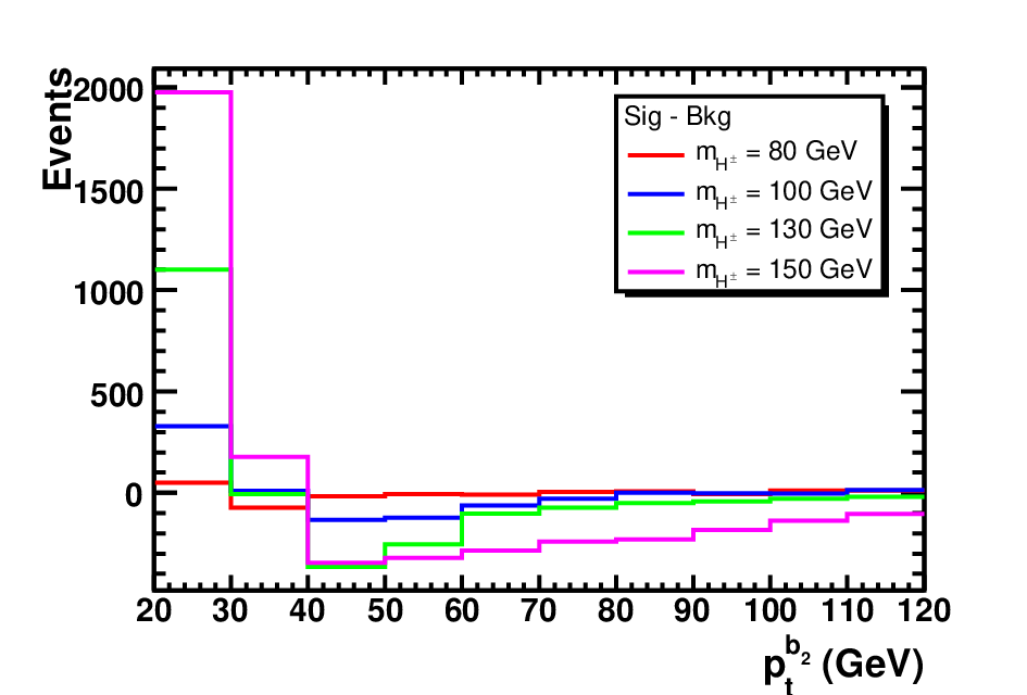
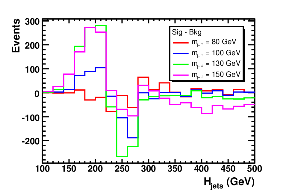
Figures 1–8 show examples of the signal and background distributions of some of the kinematic variables used in the IDA method and the respective difference between signal and background distributions, namely:
- •
the transverse momentum of the jet, (Fig. 1),
- •
the transverse momentum of the leading in the jet, (Fig. 2)
- •
the ratio (Fig. 3),
- •
the transverse momentum of the second (least energetic) quark jet, (Fig. 4),
- •
the transverse mass in the system, , where is the azimuthal angle between and (Fig. 5)44 4 Strictly speaking this is not the transverse mass since there are two neutrinos in the decay chain of the charged Higgs boson we are considering, even so the characteristics of this mass are very similar to that of the true transverse mass.,
- •
the invariant mass distribution of the two light quark jets and the second quark jet, (Fig. 6),
- •
the spatial distance between the jet and the second quark jet, , where is the azimuthal angle between the and jet (Fig. 7) and
- •
the sum of the (scalar) transverse momenta of all the quark jets, (Fig. 8).
The distributions of signal and background events are normalized to the same number of events, in order to make small differences better visible.
The signal and background distributions for the variables shown in Figs. 4–8 are as expected rather similar for and are hence mostly important to discriminate between signal and background in the IDA for . Especially the transverse mass, Fig. 5, shows a large variation with the charged Higgs boson mass. However, the different spin of the charged Higgs boson and the boson has a large effect on the jet variables and (Figs. 1 and 2) resulting in significantly different distributions of signal and background even for . Moreover, the spin effects in the and distributions are correlated which can be seen in Fig. 3 where the distributions of the ratio [26, 28, 29] show even larger differences. This highlights the importance of the additional variable (and hence ), compared to a previous study [33]. The large separation power of this variable is indeed due to the different polarizations in signal and background as can be inferred from the lower plots in Figs. 1–3. There the signal and background distributions for , and are shown for reference samples where the decay has been performed without the inclusion of spin effects with the built-in routines of PYTHIA and hence the differences between signal and background nearly vanish.
2.4 Iterative Discriminant Analysis (IDA)
The IDA method is a modified Fisher Discriminant Analysis [37] and is characterized by the use of a quadratic, instead of a linear, discriminant function and also involves iterations in order to enhance the separation between signal and background.
In order to analyze our events with the IDA method, signal and background have been split in two samples of equal size. With the first set of samples the IDA training has been performed and then the second set of samples has been analyzed. We have used the following 20 variables in the IDA study: the transverse momenta , , , , , , , ; the transverse mass ; the invariant masses , , , and ; the spatial distances , , , ; the total transverse momenta of all quark jets and of all jets . In the analysis of real data, b-quark tagging probabilities and the reconstruction of and masses could be used to improve the jet pairing, and replace the allocation of least and most energetic -jet by a probabilistic analysis.
The results of the IDA study are shown in Figs. 9 and 10 for the event samples with spin effect in the decays for GeV and for the reference samples without the spin effect for GeV in order to illustrate the spin effect. In all plots of the IDA output variable the number of background events has been normalized to the number of signal events. Two IDA steps have been performed. Figure 9 shows the IDA output variable after the first step, where 90% of the signal is retained when a cut at zero is applied. The signal and background events after this cut are then passed to the second IDA step. Figure 10 shows the IDA output variable distributions after the second step. A cut on these distributions leads to the efficiency and purity (defined as ratio of the number of signal events divided by the sum of signal and background events) combinations as shown in the lower right plot in Fig. 10. These combinations define the working point (number of expected background events for a given signal efficiency) and the latter can be optimized to maximize the discovery potential. The difference between the dashed (no spin effects in decay) and solid (with spin effects in decay) lines for GeV in the lower right plot in Fig. 10 stresses again the importance of the spin effects to separate signal and background.
In order to illustrate the effect of the hard cut on the missing transverse momentum ( GeV), which is imposed to suppress the QCD background, the final efficiency-purity plot of the IDA analysis is shown in Fig. 11 for GeV for two reference samples (red, long dashed: with spin effects in the decay; red, dotted: without spin effects) without imposing the hard cut. The black lines (dashed and solid) are for the samples with the hard cut as also shown in the lower right plot in Fig. 10. As expected the achievable purity for a given efficiency decreases with the hard cut, therefore the spin effects become even more important to separate signal and background. In principle, by choosing the signal reduction rates in the previous IDA iterations, the signal and background rates in the final distributions can be varied appropriately. However, we have checked that a different number of IDA iterations and/or different efficiencies for the first IDA iteration have only a minor effect on the final result.






3 LHC ENERGY
The simulation procedure and the emulation of the detector response are the same as those outlined in Sect. 2.1 for the Tevatron, as well as, for the preselection and IDA method, as described in Sects. 2.3 and 2.4, respectively. Hence, only the expected LHC rates are discussed, followed by the description of changes in the distributions of the variables and the final IDA results.
Unlike the case of the Tevatron, where only charged Higgs masses smaller than the top quark mass can be explored, and 2HDM/MSSM signatures practically rely on pairs only, at the LHC the phenomenology is more varied. Here, the search strategies depend strongly on the charged Higgs boson mass. If (later referred to as a light Higgs boson), the charged Higgs boson can be produced in top (anti-)quark decay. The main source of top (anti-)quarks at the LHC is again pair production ( pb at NLO) [38]. For the whole () parameter space there is a competition between the and channels in top decay keeping the sum at almost unity. The top quark decay to is however the dominant mode for most of the parameter space. Thus, the best way to search for a (light) charged Higgs boson is by requiring that the top quark produced in the process decays to a . While in the case of decays ’s will be tagged via their hadronic decay producing low-multiplicity narrow jets in the detector, there are two different decays that can be explored. The leptonic signature provides a clean selection of the signal via the identification of the lepton . In this case the charged Higgs transverse mass cannot be reconstructed because of the presence of two neutrinos with different origin. In this channel charged Higgs discovery will be determined by the observation of an excess of such events over SM expectations through a simple counting experiment. In the case of hadronic decays the transverse mass can instead be reconstructed since all neutrinos are arising from the charged Higgs boson decay. This allows for an efficient separation of the signal and the main background (assuming ). The absence of a lepton ( or ) provides a less clean environment but the use of the transverse mass makes it possible to reach the same mass discovery region as in the previous case and also to extract the charged Higgs boson mass. Both these channels show that after an integrated luminosity of 30 fb-1 the discovery could be possible up to a mass of 150 GeV for all tan values in both ATLAS and CMS [9, 39, 40].
If the charged Higgs is heavier than the top quark, the dominant decay channels are and depending on . They have both been studied by ATLAS and CMS [41, 42, 43, 44]. The charged Higgs bosons are produced in the channel. For the decay, a charged Higgs boson can be discovered up to high masses ( GeV) in the case of very large values and this reach cannot be much improved because of the large multi-jet environment. For the decay mode this reach is larger due to a cleaner signal despite a lower BR. In this case the 5 reach ranges from for GeV to for GeV.
For the LHC, signal and background events have been simulated in the same way as for the Tevatron as described before, however, without implying any rescaling factor to match a measured cross section. Table 2 lists the resulting cross sections before () and after () applying the basic cuts GeV and the hard cut GeV. The LHC rates allow for the discovery to be less challenging than at the Tevatron in the region , yet the separation of signal events from background remains crucial for the measurement of the charged Higgs mass.
| (GeV) | 80 | 80 | 100 | 130 | 150 |
|---|---|---|---|---|---|
| (pb) | 45.5 | 72.6 | 52.0 | 24.5 | 9.8 |
| (pb) for GeV | 17.3 | 33.9 | 25.7 | 12.2 | 3.8 |
| (pb) for GeV | 4.6 | 6.0 | 4.8 | 2.9 | 1.2 |
The kinematic distributions are shown in Figs. 12 to 19 for TeV. The choice of variables is identical to the one for the Tevatron and allows for a one-to-one comparison, the differences being due to a change in CM energy (and, to a somewhat lesser extent, due to the leading partonic mode of the production process55 5 As the latter is dominated by annihilation at the Tevatron and fusion at the LHC.). The main differences with respect to Figs. 1–8 are that the various transverse momenta and invariant masses have longer high energy tails. In particular, it should be noted that the effect of the spin differences between and events can be explored very effectively also at LHC energies, e.g. the ratio is shown in Fig. 14 which is very sensitive to the spin effects. These observations lead to the conclusion that the same method using spin differences can be used to separate signal from background at both the Tevatron and the LHC.
The distributions of the IDA output variables for the study at TeV for two steps with 90% efficiency in the first step are shown in Figs. 20 and 21. These distributions are qualitatively similar to those for the Tevatron (Figs. 9 and 10) and the final achievable purity for a given efficiency is shown in Fig. 21. As for the Tevatron energy a good separation of signal and background events can be achieved with the spin sensitive variables and the IDA method even in case . For heavier masses the separation of signal and background events increases due to the kinematic differences of the event topology.
4 CONCLUSIONS
The discovery of charged Higgs bosons would be a clear sign of physics beyond the SM. In this case study we have investigated charged Higgs boson topologies produced at the current Tevatron and LHC energies and compared them against the irreducible SM background due to top-antitop production and decay. While sizable differences between signal and background are expected whenever , near the current mass limit of about GeV the kinematic spectra are very similar between SM decays and those involving charged Higgs bosons. In this case, spin information will significantly distinguish between signal and irreducible SM background. In fact, we have considered hadronic decays of charged Higgs bosons, wherein the polarization induced by a decaying (pseudo)scalar object is significantly different from those emerging in the vector () decays onsetting in the top-antitop case. For a realistic analysis which is not specific for a particular detector, a dedicated Monte Carlo event generation and a simplified multipurpose detector response approximation have been applied. The identification of a hadronic tau-lepton will be an experimental challenge in an environment with typically four jets being present. We have demonstrated how an IDA method can be an applied to separate signal and background when the differences between the signal and background distributions are small. Our results show that the IDA method will be equally effective at both the Tevatron and LHC. While only the dominant irreducible background has been dealt with in detail, we have also specifically addressed the QCD background. A suitably hard missing transverse momentum cut has been applied to reject such jet activity and we have demonstrated that although the discriminative power is reduced by such a cut, the reduction is small compared to the gain from including the polarization effects. Using the differences in polarization between the signal and the dominant SM irreducible background is crucial for disentangling the former from the latter.
ACKNOWLEDGMENTS
We would like to thank the organizers of the 2005 and 2007 editions of the Les Houches workshops “Physics at TeV Colliders’ (where part of this work was carried out) for their kind invitation and Johan Alwall for fruitful discussions. SH and AS thank the Department of Nuclear and Particle Physics, Uppsala University, for hospitality and financial support during the Charged2006 workshop where part of this work was carried out. SM thanks The Royal Society (London, UK) for partial financial support in the form of a ‘Conference Grant’ to attend all the aforementioned workshops.
References
- [1] A. Sopczak, Int. J. Mod. Phys. A 9, 1747 (1994).
- [2] A. Sopczak, Z. Phys. C 65, 449 (1995).
- [3] M. Carena, J.S. Conway, H.E. Haber and J.D. Hobbs (conveners), Proceedings of the ‘Tevatron Run II SUSY/Higgs’ Workshop, Fermilab, Batavia, Illinois, USA, February-November 1998, preprint Fermilab-Conf-00/279-T and SCIPP-00/37, October 2000, hep-ph/0010338.
- [4] K.A. Assamagan, A. Djouadi, M. Drees, M. Guchait, R. Kinnunen, J.-L. Kneur, D.J. Miller, S. Moretti, K. Odagiri and D.P. Roy, in Proceedings of the Workshop ‘Physics at TeV Colliders’, Les Houches, France, 8-18 June 1999, preprint January 2000, hep-ph/0002258.
- [5] J.F. Gunion, H.E. Haber, G.L. Kane and S. Dawson, “The Higgs Hunters’ Guide” (Addison-Wesley, Reading, MA, 1990); A. Djouadi, hep-ph/0503172 and hep-ph/0503173.
- [6] D. P. Roy, Mod. Phys. Lett. A 19, 1813 (2004).
- [7] D. P. Roy, hep-ph/0409201.
- [8] D. P. Roy, hep-ph/0510070.
- [9] B. Mohn, M. Flechl and J. Alwall, ATL-PHYS-PUB-2007-006.
- [10] ALEPH, DELPHI, L3 and OPAL [The LEP Higgs Working Group for Higgs boson searches], hep-ex/0107031.
- [11] J. Alwall, C. Biscarat, S. Moretti, J. Rathsman and A. Sopczak, Eur. Phys. J. C 39S1, 37 (2005).
- [12] F. Borzumati, J.-L. Kneur and N. Polonsky, Phys. Rev. D 60, 115011 (1999).
- [13] D.J. Miller, S. Moretti, D.P. Roy and W.J. Stirling, Phys. Rev. D 61, 055011 (2000).
- [14] S. Moretti and D. P. Roy, Phys. Lett. B 470, 209 (1999).
- [15] D. Cavalli et al., hep-ph/0203056.
- [16] K. A. Assamagan et al., hep-ph/0406152.
- [17] M. Guchait and S. Moretti, JHEP 0201, 001 (2002).
- [18] S. Moretti, Pramana 60, 369 (2003).
- [19] K. A. Assamagan, M. Guchait and S. Moretti, hep-ph/0402057.
- [20] G. Marchesini, B.R. Webber, G. Abbiendi, I.G. Knowles, M.H. Seymour and L. Stanco, Comp. Phys. Commun. 67, 465 (1992).
- [21] G. Corcella et al., JHEP 0101, 010 (2001).
- [22] G. Corcella et al., hep-ph/0210213.
- [23] S. Moretti, K. Odagiri, P. Richardson, M.H. Seymour and B.R. Webber, JHEP 0204, 028 (2002).
- [24] T. Sjöstrand, Comp. Phys. Comm. 82, 74 (1994); T. Sjöstrand, P. Edén, C. Friberg, L. Lönnblad, G. Miu, S. Mrenna and E. Norrbin, Comp. Phys. Commun. 135, 238 (2001); T. Sjöstrand, L. Lönnblad and S. Mrenna, hep-ph/0108264; T. Sjostrand, L. Lonnblad, S. Mrenna and P. Skands, hep-ph/0308153.
- [25] J. Alwall and J. Rathsman, JHEP 0412, 050 (2004).
- [26] D. P. Roy, Phys. Lett. B 277, 183 (1992).
- [27] S. Raychaudhuri and D. P. Roy, Phys. Rev. D 52, 1556 (1995).
- [28] S. Raychaudhuri and D. P. Roy, Phys. Rev. D 53, 4902 (1996).
- [29] D. P. Roy, Phys. Lett. B 459, 607 (1999).
- [30] K. A. Assamagan and Y. Coadou, Acta Phys. Polon. B 33, 707 (2002).
- [31] K. A. Assamagan, Y. Coadou and A. Deandrea, Eur. Phys. J. directC 4, 9 (2002).
- [32] V. M. Abazov et al. [DØ Collaboration], Phys. Rev. D 71, 072004 (2005).
- [33] V. Bunichev, L. Dudko, S. Hesselbach, S. Moretti, S. Perries, J. Petzoldt, A. Pompoš, J. Rathsman and A. Sopczak, in “Les Houches ”Physics at TeV Colliders 2005” Beyond the Standard Model working group: summary report”, hep-ph/0602198.
- [34] S. Jadach, J. H. Kuhn and Z. Was, Comput. Phys. Commun. 64, 275 (1990).
- [35] P. Golonka, B. Kersevan, T. Pierzchala, E. Richter-Was, Z. Was and M. Worek, hep-ph/0312240.
- [36] DØ Collaboration, DØ note 4879-CONF, 12th September 2005.
- [37] J. Malmgren and K. Johansson, Nucl. Inst. Methods A 403 (1998) 481.
- [38] M. Beneke et al., hep-ph/0003033.
- [39] C. Biscarat and M. Dosil, ATL-PHYS-2003-038.
- [40] S. Abdullin et al., CMS Note 2003/033.
- [41] K.A. Assamagan and N. Gollub, SN-ATLAS-2004-042.
- [42] R. Kinnunen, CMS Note 2000/039.
- [43] P. Salmi, R. Kinnunen and N. Stepanov, CMS Note 2002/024.
- [44] S. Lowette, J, Heyninck and P. Vanlaer, CMS Note 2004/017.