Driven waves in a two-fluid plasma
Abstract
We study the physics of wave propagation in a weakly ionised plasma, as it applies to the formation of multifluid, MHD shock waves. We model the plasma as separate charged and neutral fluids which are coupled by ion-neutral friction. At times much less than the ion-neutral drag time, the fluids are decoupled and so evolve independently. At later times, the evolution is determined by the large inertial mismatch between the charged and neutral particles. The neutral flow continues to evolve independently; the charged flow is driven by and slaved to the neutral flow by friction. We calculate this driven flow analytically by considering the special but realistic case where the charged fluid obeys linearized equations of motion. We carry out an extensive analysis of linear, driven, MHD waves. The physics of driven MHD waves is embodied in certain Green functions which describe wave propagation on short time scales, ambipolar diffusion on long time scales, and transitional behavior at intermediate times. By way of illustration, we give an approximate solution for the formation of a multifluid shock during the collision of two identical interstellar clouds. The collision produces forward- and reverse J shocks in the neutral fluid and a transient in the charged fluid. The latter rapidly evolves into a pair of magnetic precursors on the J shocks, wherein the ions undergo force free motion and the magnetic field grows monotonically with time. The flow appears to be self similar at the time when linear analysis ceases to be valid.
Keywords:
diffusion — MHD — waves — shock waves — ISM: magnetic fields — ISM: clouds1 Introduction
It is well known that shock waves in weakly-ionised interstellar plasmas have a multifluid structure, where the charged and neutral components of the plasma behave as separate, interacting fluids (Mullan 1971). Because their multifluid nature has profound observational consequences (Draine 1980), multifluid shocks have been the subject of numerous studies on their structure, chemistry, and emission (last reviewed by Draine & McKee 1993). Although the majority of these studies have assumed steady flow, a small fraction have carried out time dependent simulations, either to follow the development of instabilities (Mac Low & Smith 1997; Stone 1997; Neufeld & Stone 1997) or to study evolutionary effects (Smith & Mac Low 1997; Chièze, Pineau des Forêts & Flower 1998; Ciolek & Roberge 2002; Lesaffre et al. 2004a,b).
This paper describes the formation of a multifluid shock wave by a sudden disturbance, e.g., the collision of two cloud cores or the impact of a protostellar outflow onto surrounding core material. We focus on time scales , where the ion-neutral drag time, , is the slowing-down time for an ion drifting through a neutral gas. This is a very short time: yr in a typical dense core (§2). Nevertheless, there are good reasons for studying this extremely brief, unobservable period. First, the physics is interesting. The response of a plasma to a sudden disturbance depends on the wave modes it supports over a broad range in frequency, . In a weakly ionised plasma the allowed modes represent propagating waves if and diffusion if (§3.3). We wish to understand how these qualitatively different behaviors manifest themselves at early times, and whether the resulting effects influence the flow at later, observable times. Second, the present study serves as a prototype for future work, on the effects of charged dust grains on multifluid shocks. These effects are known to be important (Wardle 1998; Ciolek & Roberge 2002; Ciolek, Roberge & Mouschovias 2004; Chapman & Wardle 2006). Including dust will be analogous in some ways to the present study, but dust also adds new physics and a higher level of complexity to the problem. Third, the results of this paper have practical use. As a computational expedient, some time dependent simulations of multifluid shock waves neglect the inertia of the charged fluid (e.g., Smith & Mac Low 1997). Since the inertia is important on precisely the time scales studied here, the present work provides benchmark tests on this assumption.
The plan of this paper is as follows. In §2 we give the equations of motion for a time dependent, multifluid shock wave in a form which exploits the small time scale of interest. In §3 the linearized versions of these equations (§3.1) are presented and we discuss the allowed wave modes (§§3.2–3.3). We emphasize that linear analysis yields highly accurate solutions for some special but realistic cases; the general case will be studied numerically in a separate paper. Analytical methods for calculating the time dependent flow of charged and neutral particles are described in §§3.4–3.9. These techniques are used in §4 to find an approximate solution for the formation of a multifluid shock during the collision of two identical clouds. Our results are summarized in §5.
2 Governing Equations
We are interested in the multifluid flow which ensues when a weakly ionized plasma is accelerated and compressed by a sudden disturbance. We model the plasma as separate charged and neutral fluids which interact via elastic scattering. The charged fluid is composed of ions and electrons (the effects of charged dust grains will be considered in a separate paper) plus a magnetic field which is everywhere frozen into the charged fluid. We adopt planar geometry with the magnetic field along the direction and fluid velocities along the directions.
The equations of motion for an arbitrary disturbance in a two-fluid plasma were derived by Draine (1986; see also Nemirovsky, Fredkin & Ron 2002). Here we solve modified versions of these equations which take advantage of the extremely short time scale— typically less than yr— on which we follow the flow. The charged fluid is described by the equations of mass conservation, momentum conservation, and the induction equation:
| (1) |
| (2) |
and
| (3) |
respectively, where and are the density and velocity of the charged fluid, is the velocity of the neutral fluid, and is the magnetic field. The first term on the RHS of eq. (2) is the frictional acceleration produced by elastic scattering between ions and neutral particles and the second is the acceleration caused by the magnetic pressure gradient.
The characteristic time scale for acceleration by friction is the ion-neutral drag time, . If the charged and neutral fluids were each composed of a single species, then
| (4) |
where and are the neutral and ion particle masses, respectively, is the number density of the neutral fluid, and is the momentum transfer rate coefficient for elastic ion-neutral scattering. For a typical cloud core with cm-3 and , one finds yr. This is a fundamental time scale for the flow.
We have omitted the energy equation for the charged fluid because eq. (1)–(2) are independent of the ion and electron temperatures, and . This is appropriate at the very low fractional ionizations of interest here, where the pressure of the charged fluid is dominated by magnetic pressure. The cooling rate of the neutral fluid generally depends on and (via the rates of ion- and electron impact processes) but we assume that radiative cooling is negligible on the time scales of interest. For a gas with cm-3, the cooling time is yr if the neutral temperature is less than K. In eq. (1) we have omitted a term which represents mass transfer between the charged and neutral fluids. This is always a good approximation because the recombination time scale is always yr in dense clouds.
We assume that the neutral fluid is governed by Euler’s equations for adiabatic flow,
| (5) |
| (6) |
and
| (7) |
Mass transfer in eq. (5) is also neglected, for reasons noted above. We have neglected momentum transfer by friction in eq. (6) because the time for friction to accelerate the neutral fluid is
| (8) |
or about yr in a dense core.11 1 Of course this means that the total momentum of the charged plus neutral fluids is not conserved but the associated error is . We have also neglected heating of the neutral fluid by ion-neutral friction and the associated acceleration by thermal pressure gradients; one can show that these effects are small on time scales yr.
The equations of motion for the charged fluid depend on the neutral velocity, , and number density, . In the next section, on the dynamics of the charged fluid, we assume that and are known functions of and which have been determined by solving Euler’s equations. How this all works out for a particular example is demonstrated in §4.
3 The Physics of Driven Waves
3.1 Linearized Equations of Motion
We follow the flow of the charged fluid by solving the linearized versions of eq. (1)–(3). This is an expedient which allows us to work the problem analytically. Our analytical solutions reveal the essential physics; numerical solutions of the full nonlinear equations will be discussed elsewhere. However it is important to note that linear theory is highly accurate for some initial conditions at sufficiently short times; this is ultimately because the speed of a typical disturbance (– km s-1) is much smaller than the ion Alfvén speed ( km s-1). A specific example is discussed in §4.
The zero-order solution of eq. (1)–(3) is a spatially uniform state in which the charged fluid has constant density , magnetic field, , and zero velocity. Onto the zero-order state we superpose density, magnetic field, and velocity perturbations denoted , , and , respectively. We adopt dimensionless perturbations so that
| (9) |
| (10) |
and
| (11) |
where
| (12) |
is the ion Alfvén speed in the zero-order state. We also adopt dimensionless time and distance units. In all subsequent discussion, is dimensionless time in units of and is dimensionless distance in units of . In this paper we shall assume that is independent of and . This allows us to obtain analytical solutions but, because depends on the density of the neutral fluid, only hypothetical flows with uniform density can be studied analytically.
Linearizing eqs. (1)–(3) about the zero-order solution gives the equations of motion:
| (13) |
| (14) |
and
| (15) |
where
| (16) |
and the dots and primes denote partial derivatives with respect to and , respectively. We seek solutions of equations (13)–(15) subject to the initial conditions
| (17) |
| (18) |
and
| (19) |
where , , and are small but otherwise arbitrary functions. We assume that has been determined as described in §2. For the purposes of this section it is a known, small, but otherwise arbitrary function.
3.2 Fourier Analysis
To proceed we Fourier transform eq. (13)–(15) to eliminate the spatial derivatives. We define the Fourier transform of by
| (20) |
Writing the perturbations as Fourier integrals transforms eq. (13)–(15) into a set of linear, inhomogeneous, coupled, ODEs for the transforms of the perturbations:
| (21) |
where the vector of unknowns is
| (22) |
the coupling matrix is
| (23) |
and the source term,
| (24) |
represents the effects of frictional driving.
Equation (21) can be solved by standard methods. The solution has the form
| (25) |
where the particular solution, , is any solution of eq. (21) and the homogeneous solution, , is any solution with . The “total” solution must satisfy the initial conditions
| (26) |
but there is a degree of arbitrariness in how the right side of (26) is apportioned between the particular and homogeneous parts on the left. We require
| (27) |
and
| (28) |
Then for a given set of initial conditions, the homogeneous solution represents the disturbance that would occur, for the same initial conditions, if the driving force was zero. We show in §3.3 that the homogeneous solution has no growing modes; it is therefore entirely transient in nature. The particular solution always has a transient component but may also contain a steady part if the driving is steady (see §3.9).
3.3 Dispersion Relations
The solution of eq. (21) depends on the eigenvalues and eigenvectors of the coupling matrix. It is easy to show that has three eigenvalues, , , and , where
| (29) |
and
| (30) |
The corresponding eigenvectors are
| (31) |
and
| (32) |
respectively.

The eigenvalues and eigenvectors depend on the complex-valued function
| (33) |
where is the dimensionless22 2 In ordinary units, , where is the maximum wavelength for propagating ion magnetosound (and Alfvén) waves in a cold plasma (Kulsrud & Pearce 1969; Ciolek, et al. 2004). “critical wave number.” For real the meaning of is ambiguous on the interval , where has a branch cut in the complex plane (Fig. 1). We will take
| (34) |
where “” denotes the positive square root. This means that for real we evaluate “just above” the branch cut, a fact which becomes crucial when Fourier transforms are evaluated as contour integrals (App. A). With our definition of , the dependence of and on (for real ) is as shown in Fig. 3–3. Kulsrud and Pearce (1969) found the analogous dispersion relations for Alfvén waves in a cold ion-neutral plasma. For dimensionless wave numbers , where the neutrals act as a stationary background, their dispersion relation reduces to expression (30) for [cf. Kulsrud & Pearce 1969, eq. (C7)].


The physics of the different wave modes is well understood but worth repeating for later discussion. The mode represents perturbations (e.g., perturbations in ) that move along with the charged fluid. For the and modes represent propagating waves (Fig. 3). For very large wave numbers, the dispersion relations become
| (35) |
In this limit the phase velocity approaches ( in ordinary units) and the damping time approaches ().
For the and modes are both evanescent (Fig. 3). However they describe qualitatively different behavior. For very small wave numbers the dispersion relations become
| (36) |
and
| (37) |
These are to be compared with the dispersion relation
| (38) |
for the diffusion equation with diffusion coefficient . Evidently represents diffusion with and zero damping. This “diffusion mode” dominates all solutions at large times. In contrast, represents “antidiffusion” with and strong damping. The mode describes the transient compression of which can occur at early times for some initial conditions. However it is never important for .
3.4 Homogeneous Solution
The homogeneous solution of eq. (21) is
| (39) |
where summation is implied by the repeated index. The coefficients are functions of but not time and are determined by the initial conditions. Setting in eq. (39) and substituting the result into the LHS of eq. (28) gives a set of linear algebraic equations for . The solution is
| (40) |
| (41) |
and
| (42) |
The expansion coefficients obey the symmetry requirement under the interchange . To see this, note that [cf. eq. (30)].
The transforms of the perturbations are obtained by substituting the expansion coefficients into eq. (39). After lengthy algebra we find that
| (43) |
| (44) |
and
| (45) |
We have introduced the function
| (46) |
where
| (47) |
and
| (48) |
and are the Fourier transforms of and , respectively. We shall see shortly that , , and are the Fourier transforms of certain Green functions. The Green functions are calculated in Appendix A and discussed in §3.6. Here we simply note that they are causal:
| (49) |
The homogeneous solution for the perturbations is obtained by taking the inverse Fourier transforms of expressions (43)–(45). This can be done by inspection using the Convolution Theorem,
| (50) |
The result is the homogeneous solution:
| (51) |
| (52) |
and
| (53) |
where the angle brackets signify convolution,
| (54) |
and causality has been used to refine the limits of integration.
Expression (51) for the density perturbation has a simple physical interpretation. Taking the ratio of eq. (10) and (9) and neglecting terms of second order gives
| (55) |
But according to eq. (51), the factor in square brackets is a conserved quantity so
| (56) |
Noting that in the unperturbed state, we see that expression (56) implies flux freezing. Of course flux freezing was put into the solution a priori, so there was really no need to calculate the density perturbation independently of the magnetic field perturbation. However it is reassuring to know that the homogeneous solution is self consistent in this respect.
3.5 Particular Solution
The particular solution of eq. (21) has the form
| (57) |
where the coefficients generally depend on time as well as . One can verify that expression (57) is a solution of eq. (21) provided
| (58) |
Expression (58) is a set of coupled ODEs for with initial conditions
| (59) |
The solution is
| (60) |
| (61) |
and
| (62) |
Substituting the expansion coefficients into expression (57) yields the Fourier transforms of the perturbations. The inverse transform then yields the particular solution:
| (63) |
| (64) | |||||
and
| (65) | |||||
where the Convolution Theorem has been used again. Comparing eq. (63) to eq. (51) and noting that the particular solution vanishes at , we see that the particular solution also incorporates flux freezing. Since flux freezing uniquely relates the density perturbation to the magnetic field perturbation, we omit further discussion of .
3.6 Green Functions

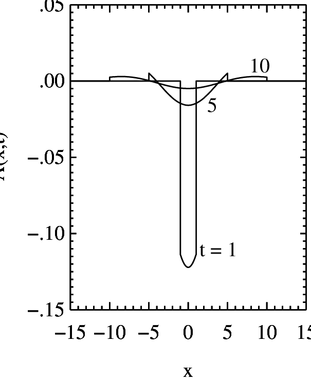

The Green function is calculated in Appendix A. We find that
| (66) |
where it the modified Bessel function of order zero,
| (67) |
and the rectangle function,
| (68) |
insures causality. In Fig. 4 we plot vs. at selected times.
Differentiating yields the other Green functions,
| (69) |
and
| (70) |
where
| (71) |
and
| (72) |
It is useful to know the normalization of the Green functions (e.g., to check the numerical evaluation of convolution integrals). It is easy to show that
| (73) |
| (74) |
and
| (75) |
3.7 Large Time Behavior
The discussion of the dispersion relations (§3.3) suggests that diffusion dominates the physics on large length scales. Because the damping rate of the diffusion mode increases with (Fig. 3), this should be reflected in the large-time behavior of the Green functions. In Appendix B we show that
| (76) |
Consistent with the discussion in §3.3, approaches the Green function for the diffusion equation with unit diffusion coefficient. We also show in App. B that the other Green functions are smaller than at large times, with
| (77) |
(see Fig. 7).
The asymptotic forms of the Green functions lead to a particularly simple result for the solution when driving is absent. If one replaces with and uses expression (77) to omit all but the nonvanishing terms of largest order in the homogeneous solution, the latter becomes
| (78) |
and
| (79) |
Equation (78) indicates that the magnetic field satisfies a diffusion equation when , as expected. Equation (79) is understood by noting that
| (80) |
so that eq. (79) is the same thing as
| (81) |
The last expression says that the magnetic and drag forces on the charged fluid balance one another [cf. eq. (15) with ]. This is also expected: when , the inertia of the ions becomes negligible and they undergo force-free motion.

3.8 Small Time Behavior
When , the effects of friction are small and the results of §3 for driven waves should reduce to the corresponding results for ideal MHD. The latter can be found in a form suitable for comparison by setting in the linearized momentum equation and retracing the steps leading to eq. (51)–(53) (for the homogeneous solution) and eq. (63)–(65) (particular solution). The calculation is very straightforward and we simply give the results:
| (82) |
and
| (83) |
where the “frictionless Green functions” are
| (84) |
and
| (85) |
We wish to compare expressions (82) and (83) to the corresponding solution with friction in the limit . The particular solution obviously goes to zero as . To find the limit of the homogeneous solution, we note that any convolution integral approaches zero if its kernel is , , or , because the amplitude of each of these functions remains finite as , and is zero for . Retaining only the delta function kernels (with for ) is equivalent to making the replacements
| (86) |
| (87) |
and
| (88) |
in eq. (52)–(53). This shows that the physics of driven waves reduces to ideal MHD in the appropriate limit.

A comparison of the Green functions for waves with and without friction also shows how ion-neutral friction alters the physics of wave propagation. This is best illustrated by examining the solutions in terms of the Riemann invariants,
| (89) |
and
| (90) |
In terms of and the solution for ideal MHD becomes
| (91) |
and
| (92) |
where we have used the fact that
| (93) |
to evaluate the convolutions. The analogous solution for driven waves is
| (94) |
and
| (95) |
Expressions (91) and (92) say that the Riemann invariants are conserved quantities in ideal MHD. The former is transported along the characteristic curve and the latter along (Fig. 8). It follows that the solution at each spacetime point depends only on the initial conditions at the points and (Fig. 8). This is the essence of wave propagation. When friction is present, the situation is similar yet not identical. The first term on the RHS of eq. (94) and eq. (95) may be interpreted to mean that the Riemann “invariants” are still transported along characteristics, but with exponential attenuation. That is, they represent wave propagation with damping. However the presence of additional terms shows that this is not the whole story. For example, the nonzero widths of the convolution kernels on each RHS imply that the solution at depends on the initial conditions over the entire spatial interval . This is the signature of diffusion.
The physics of wave propagation, diffusion, and the transition from wavelike to diffusive behavior is apparent in the plots of the Green functions (Fig. 4–6). Wave fronts are located by the jumps at , propagating with velocities of . Diffusion is implied by the finite widths of the Green functions. The transition from wave propagation to diffusion occurs at times of order unity, when the jumps have decayed conspicuously. At much greater times the jumps become invisible and all vestiges of wave propagation disappear.
3.9 Steady Driving
The physics of driven waves simplifies dramatically when the frictional driving is steady. Since we are interested in time scales where the neutral flow is approximately steady, it is worth discussing this case in some detail. Only the particular solution needs to be considered; the homogeneous solution depends only on the initial conditions, and so requires no modification.
If the neutral flow is steady then it is possible to write
| (96) |
where is the neutral velocity profile and is the pattern velocity.33 3 Note that the linearized equations of motion are not invariant under Galilean transformations: they are valid only in the frame where the undisturbed gas far upstream is at rest. The pattern velocity is evaluated in this frame. Then the Fourier transform of has the form
| (97) |
and the simple time dependence of makes it possible to find the expansion coefficients explicitly. Substituting expression (97) into equations (60) and (62) and evaluating the integrals gives
| (98) |
and
| (99) |
where
| (100) |
| (101) |
| (102) |
Having found and , we only need to calculate the inverse transform of expression (57) to find the particular solution. Evidently the latter contains two parts: terms in that are proportional to represent steady flow of the charged fluid, which must eventually result from steady driving by the neutrals. The other terms in represent the transient response to driving.
First we evaluate the velocity, . Substituting expressions (98) and (99) into eq. (57) gives
| (103) |
where
| (104) |
and
| (105) |
are the steady and transient parts, respectively. Now the inverse transform of expression (104) is
| (106) |
where
| (107) |
The inverse transform of is evaluated by simple contour integration to find
| (108) |
If we use this result and the Convolution Theorem to evaluate expression (106), we obtain the steady part of the ion velocity:
| (109) |
where
| (110) |
This is a remarkably simple result. If the neutral flow is steady, then the charged fluid will eventually undergo steady flow with the same pattern velocity, consistent with common sense. When both flows are steady, the velocity of the charged fluid is just the convolution of the driving force, , with an exponential response function, .
Now consider the transient part of the ion velocity. Substituting expressions (100)–(102) into equation (105), we find after routine algebra that
| (111) |
Inverting the transform is performed by a twofold application of the Convolution Theorem once the inverse transforms of and are known. We find that
| (112) |
and
| (113) |
Using these results and the Convolution Theorem yields
| (114) |
The transform of the magnetic field perturbation is
| (115) |
The inverse transforms are obtained by steps very similar to those used to find the velocity. We omit the details and simply state the result:
| (116) | |||||
4 A Cloud-Cloud Collision
As an application of the methods developed in §3, we consider the collision of two identical, uniform, semi-infinite clouds. The relative motion is taken to be along and the magnetic fields to be everywhere along . Prior to the collision the free surface of each cloud is a plane normal to . The collision occurs at , when the free surfaces touch at the contact discontinuity, . We take the relative velocity of the clouds to be km s-1 and adopt initial conditions appropriate for a dense core: the neutral fluid in each cloud is pure molecular hydrogen with cm-3, the charged fluid has amu, , and the unperturbed magnetic field is G. Then the characteristic speeds, time- and length scales are km s-1, yr, yr, and cm.
The homogeneous solution depends only on the initial conditions, which are
| (117) |
for the density and field perturbations. We adopt a reference frame (the “CM frame”) where the clouds approach with equal and opposite velocities. In this frame the initial velocity perturbation is
| (118) |
where
| (119) |
and
| (120) |
Using these initial conditions, we calculated the homogeneous solution by evaluating expressions (52) and (53).44 4 Taking care to evaluate expressions (52) and (53) in reference frames where they are valid. See footnote 3.


The particular solution depends on the velocity profile of the neutral fluid, which is determined by solving Euler’s equations. This is straightforward as the example considered here is just a special case of the Riemann problem in gas dynamics. Using the Riemann solver of Toro 1999, we calculated for an adiabatic ideal gas with . We set the temperature of the unperturbed neutral gas somewhat arbitrarily to K; that is, we did not find self-consistently by requiring thermal balance in the unperturbed state. (Since the shocks in this example are very strong, the value of hardly affects the solution.) The neutral flow is steady. It consists of forward- and reverse J shocks propagating with constant velocities in the directions. The shock velocities are km s-1 in the CM frame, corresponding to identical shock speeds of 13.3 km s-1 relative to the upstream gas. Having found , we obtained the particular solution from expressions (109), (114), and (116).
The velocity of the neutral fluid is plotted in Fig. 9 at the extremely early time ( s!). The region between the J fronts (the “g-star region”) contains neutral gas which has been swept up, heated, and compressed by the shocks. Because these shocks are very strong (with Mach numbers ), the swept-up gas is denser than the undisturbed gas by a large factor (), in gross violation of our assumption that is constant. Moreover the g-star region is so hot ( K) that radiative cooling is important even on time scales yr. In a separate paper we describe numerical calculations that allow for variations in , radiative cooling, and other (e.g., nonlinear) effects. Here we temporarily forego these complications and simply warn the reader that our example may not be correct in detail.
The velocity profile of the charged fluid at is plotted in Fig. 10. At this time the effects of friction are negligible, so the flow in Fig. 10 is just the magnetohydrodynamic analog of the flow in Fig. 9. The MHD flow has a growing “m-star region” bounded on either side by a moving J front. In both the gas dynamic and MHD flows, a particle of fluid passing through a J front is brought to rest by an impulsive force inside the front; the force is collisional in the first case and magnetic in the second. In the gas dynamic flow, the collisional force vanishes outside the J fronts so the neutral fluid remains at rest inside the g-star region (Fig. 9). In the MHD flow, the magnetic force vanishes outside the J fronts but friction does not. The charged fluid appears to be at rest in the m-star region (Fig. 10) only because .
The magnetic field at is plotted in Fig. 11. The m-star region is conspicuous as a “magnetic core” of compressed fluid and magnetic field centered on the contact discontinuity. The compression is approximately uniform because the velocity gradient in the m-star region is approximately zero. The compression ratio is small () because the “shocks” in the charged fluid have ion Alfvén Mach numbers of only . Consistent with the linear analysis, the velocity jumps ( km s-1) and magnetic field jumps ( G) obey the relation
| (121) |
for linear magnetosound waves. We note also that the mathematical approach we have adopted treats discontinuities exactly (i.e., without smoothing) and that discontinuties propagate at the correct speeds.


Figures 12–14 describe the flow at ( s), when the J fronts are at cm in the neutral fluid and cm in the charged fluid. Departures from ideal MHD are now visible as slight reductions in (to km s-1) and (to G). The ions inside the m-star region are moving. They flow toward the contact discontinuity with km s-1 just downstream from the J fronts, decreasing to at (Fig. 13). The compression inside the m-star region is no longer uniform; however the density/magnetic field gradient is almost constant, with and increasing toward (Fig. 14).
The qualitative properties of the flow at follow from simple physics. To see this, it is useful to note that a particle of charged fluid moving with km s-1 would travel only cm in s. Each point on the solid curves in Fig. 12–14 therefore labels a fluid particle which has not moved appreciably since . Now consider the histories of various fluid particles, starting from the initial state when the effects of friction on the flow were negligible. More specifically, consider the forces at on particles that are inside the m-star region excluding the J fronts. All of these particles have at (Fig. 10) and the magnetic force on each vanishes (Fig. 11). The friction force is small inside the g-star region () but not outside ( km s-1). Since the net force is small inside the g-star region, we expect the charged fluid there to be almost at rest at later times. This is true at (Fig. 13). The net (=frictional) force is much larger outside the g-star region; the sign of is such that the particles tend to speed up and flow toward the contact discontinuity. This explains the nonzero values and sign of at (Fig. 12).


However the preceding argument does not explain the velocity gradient in Fig. 12, which would have the opposite sign if friction was the only force at work. This is because particles close to have been accelerating longer than particles that have just emerged from the J front. The argument is incomplete because, contrary to intuition, the magnetic force is comparable to friction at . Indeed, the two forces differ by less than % (Fig. 16). The magnetic force is caused by ambipolar diffusion. The acceleration produced initially by friction produces ion motions that transport magnetic field lines toward the contact discontinuity. Now the total magnetic flux threading the m-star region is the same, at any given time, whether friction is present or not (Fig. 14).55 5 The total flux is just the flux swept up by the J fronts, which depends only on and the front velocities. The latter are whether or not friction is present. The motion of field lines toward must therefore leave a deficit of field lines farther out (relative to the frictionless case; compare the solid and dashed curves in Fig. 14). The result is a magnetic field gradient, the sign of which has the magnetic force opposing friction everywhere.
The sign of the velocity gradient in Fig. 12 can be explained as follows. The magnetic impulse delivered to a fluid particle inside a J front is proportional to . The transport of field lines away from the fronts reduces and hence . The result is a velocity gradient with the observed sign. In fact there is a feedback mechanism at work: the reduction of tends to make the velocity gradient steeper, which increases the rate of field line migration (cf. eq. 14). And so on. This explains why jumps in the fluid variables decay exponentially rather than (say) linearly with time.
As noted above, at magnetic and collisional forces are approximately equal between the advancing front and the contact discontinuity, differing by . This may seem surprising, since one might think that balance between forces could not occur for . This is because is basically the time it takes for an ion to “lose memory” of its initial state through collisions with the neutrals. It is readily shown that, in the absence of magnetic forces, the velocity of an ion in a uniform one-dimensional flow of neutrals is given by , where is the ion’s initial velocity. Approximate balance between magnetic and drag forces, however, requires only that the two forces be comparable in magnitude, yielding a residual that is much smaller than the magnitude of the individual forces themselves. Effective force-balance in the ions behind the J front is then possible when the ratio of the net (linearized) acceleration relative to the drag acceleration becomes negligible, i.e., when (see eq. [2]). Taking , where is a characteristic post-jump ion velocity, and using in this region (see Fig. 12), this condition is equivalent to . If the magnitude of the ion velocity in the post-shock region is sufficiently reduced by the magnetic impulse at the front so that , it follows that near force-balance in the ions can happen even for . This is exactly the situation that is depicted in Figs. 12 and 14: the magnetic “kick” the ions receive at the jump dramatically reduces the ion velocity, resulting in behind the front, allowing near-equality of forces in that region at (). For this case, the collisional drag of the streaming neutrals on the ions is almost enough to balance the magnetic force due to the field gradient behind the front.
The ion motion is almost but not exactly force-free at . Outside the g-star region, gas drag pulls the ions toward the contact discontinuity and the magnetic force pushes them away (Fig. 16). Because the magnetic force is slightly larger in magnitude the ions slow down, to speeds which are almost but not quite zero when they pass into the g-star region (Fig. 13). There both forces change sign (Fig. 16); the very small net force still tends to slow the ions down, allowing them to come to rest at the contact discontinuity.


Figures 17 and 18 describe the flow at three times of order unity, the largest of which is yr. The transport of field lines away from the J fronts has attenuated the latter significantly, with a corresponding increase in within the magnetic core. These figures show the earliest phase in the formation of two multifluid, MHD shock waves by the cloud-cloud collision. At , each multifluid shock is comprised of a J shock in the neutral fluid with a nascent magnetic precursor extending upstream from its J front. Although we made some unrealistic assumptions in order to work the problem analytically (no radiative cooling, independent of ), the mismatch between the time here ( yr) and the time to accelerate the neutral fluid ( yr) leaves no doubt that the solution is qualitatively correct.
One does not expect the entire (charged+neutral) flow will approach a steady configuration until much greater times yr. However it is reasonable to suppose, given the large “signal speed” in the charged fluid, that the magnetic precursors would reach a quasi-steady state at shorter times. This is clearly not the case at where, for example, the precursors are increasing in width (Fig. 17) and the magnetic flux inside the core is growing (Fig. 18). This evolving structure is determined mostly by waves propagating into the charged fluid. Thus the linear scale () is set by the steady speed of the J fronts. In mathematical terms: the solution is “mostly” the homogeneous solution, i.e., the transient response of the charged fluid to the discontinuous initial conditions. We refer to this evolutionary phase henceforth as the “ion-electron transient.” The ion-electron transient is unobservable; however it obviously affects subsequent, possibly observable, phases.
Figures 19 and 20 display the flow at three times , the largest of which corresponds to yr. Now the solution is entirely the particular (=driven) solution. The embedded neutral shocks influence the flow mainly through the neutral velocity profile, which dictates the spatial dependence of the friction force. The fact that the neutral shocks are propagating, for example, is relatively unimportant. All traces of wave physics have disappeared but the precursors are still evolving. The flow in this phase is determined by the competition between the advection of field lines inward, driven by the ion motions, and the diffusion of field lines outward, due to the resulting magnetic field gradient. The dominance of diffusion is signalled by the linear scale, which now is . We refer to this period as the “diffusion phase” of multifluid shock formation.
It would be useful to know what physical effects terminate the diffusion phase, whether this phase lasts long enough to be observable, and whether the charged flow approaches a quasi-steady configuration. Unfortunately, the solutions for cannot be discussed here because nonlinear effects start to become important (e.g., Fig. 20). Calculations in progress will use numerical methods to include nonlinearity, radiative cooling, and variations in the density of the neutral gas. We are also exploring similarity solutions (for the diffusion phase) of the nonlinear equations of motion. If a similarity solution existed, it would rule out quasi-steady flow of the charged particles. It might also reveal which physical effects usher in the next evolutionary phase. The flow in Fig. 19 and 20 certainly appears to be self-similar. It also satisfies the prerequisites: there are no boundary conditions and the system has “forgotten” its initial conditions.


5 Summary
This paper can be summarized as follows:
(i) Our objective was to understand basic physics governing the formation of multifluid, MHD shock waves from plausible initial conditions. We focused on the earliest stages of this process, which have not been explored elsewhere.
(ii) We treated the plasma as separate fluids of charged and neutral particles which are coupled by ion-neutral friction. We exploited the large inertial mismatch between the neutral and charged fluids to simplify the calculation. On time scales yr (typically), the neutral fluid evolves as if the charged particles were absent. At sufficiently early times the neutral flow can be calculated by solving Euler’s equations. The flow of the charged fluid is driven by and slaved to the neutral flow by friction.
(iii) We calculated the charged flow for special cases where the linearized equations of motion are accurate, and carried out an extensive analysis of linear MHD waves driven by friction. The physics of driven waves is embodied in certain Green functions which describe wave propagation on short time scales, ambipolar diffusion on long time scales, and transitional behavior at intermediate times.
(iv) As an illustrative example, we simulated the collision of two identical clouds with km s-1. The simulation incorporated a few unrealistic approximations. We have argued that the results are qualitatively correct and illustrate the basic physics. Realistic solutions will be presented elsewhere.
(v) We found that the formation of a multifluid shock wave proceeds through two initial phases: an “ion-electron transient” and a “diffusion phase.” In the former, the cloud-cloud collision produces J shocks in the neutral fluid which drive wavelike transients into the charged fluid. The transients quickly evolve into magnetic precursors on the J shocks, wherein the ions undergo force free motion and the magnetic field grows steadily in time. In the diffusion phase, the charged flow continues to evolve in what appears to be self similar fashion. The magnetic precursors do not become steady at the largest times we can study, which are determined by the onset of nonlinearity.
Acknowledgments
This work was supported by the New York Center for Studies on the Origins of Life (NSCORT) and the Department of Physics, Applied Physics, and Astronomy at Rensselaer Polytechnic Institute, under NASA grant NAG 5-7589. We thank the referee, Pierre Lesaffre, for a careful reading of the manuscript and for comments that improved the presentation.
References
- Chapman & Wardle (2006) Chapman J.F., Wardle, M., 2006, MNRAS, 371, 513
- Chièze et al. (1998) Chièze J.-P., Pineau des Forêts G., Flower D.R., 1998, MNRAS, 295, 762
- Ciolek & Roberge (2002) Ciolek G.E., Roberge, W.G., 2002, ApJ, 567, 947
- Ciolek, et al. (2004) Ciolek G.E., Roberge, W.G., Mouschovias, T.Ch., 2004, ApJ, 610, 781
- Draine (1980) Draine B.T., 1980, ApJ, 241, 1021
- Draine (1986) Draine B.T., 1986, MNRAS, 220, 133
- Draine & McKee (1993) Draine B.T., McKee C.F. 1993, ARA&A, 31, 373
- Kulsrud & Pearce (1969) Kulsrud R., Pearce W.P., 1969, ApJ, 156, 445
- Lesaffre et al. (2004a) Lesaffre P., Chièze J.-P., Cabrit S., Pineau des Forêts G., 2004a, A&A, 427, 147.
- Lesaffre et al. (2004b) Lesaffre P., Chièze J.-P., Cabrit S., Pineau des Forêts G., 2004b, A&A, 427, 157.
- Mac Low & Smith (1997) Mac Low, M.-M., Smith M.D., 1997, ApJ, 491, 596
- Mullan (1971) Mullan D.J., 1971, MNRAS, 153, 145
- Nemirovsky et al. (2002) Nemirovsky, R.A., Fredkin, D.R., Ron, A., 2002, PHYS REV E, 66, 066405
- Neufeld & Stone (1997) Neufeld, D.A., Stone, J.M., 1997, ApJ, 487, 283
- Smith & Mac Low (1997) Smith M.D., Mac Low, M.-M., 1997, A&A, 326, 801
- Stone (1997) Stone J.M., 1997, ApJ, 487, 271
- Toro (1999) Toro, E.F., 1999, Riemann Solvers and Numerical Methods for Fluid Dynamics, 2nd edn. Springer, Berlin
- Wardle (1998) Wardle M., 1998, MNRAS, 298, 507
- Wyld (1999) Wyld H.W., 1999, Mathematical Methods for Physicists, Perseus Books, Reading, MA
Appendix A Fourier Integrals for the Green Functions
In order to find the Green functions it is first necessary to calculate and . This involves the evaluation of certain Fourier integrals which are almost identical to integrals that appear in the Green functions for the Klein-Gordon equation. It turns out that “our” integrals can be evaluated by exactly the same technique used in the Klein-Gordon problem. In §§A.1–A.2 we closely follow the technique of Wyld (1999, see pp. 573ff).
A.1 Fourier Integral for


The function
| (122) |
can be evaluated by contour integration as follows. Noting that as , we see that
| (123) |
In the limit , the integrand in eq. (122) goes to zero exponentially in the upper plane if and in the lower plane if . It follows that we can find by integrating around the semicircular contour in Fig. 21 if or the semicirle in Fig. 22 if , and then taking the limit of infinite radius, . Because of the branch cut in it is important to remember that the horizontal part of each semicircle lies “just above” the real axis (see §3.3).

Consider first the case (Fig. 21). Since there are no singularities in the upper plane, we find immediately that
| (124) |
Now consider the case (Fig. 22). By Cauchy’s Theorem, the contour in Fig. 22 can be deformed into the one in Fig. 23 without changing the integral. If we simultaneously change variables from to , where
| (125) |
then expression (122) becomes
| (126) |
where the contour is now a line segment, as indicated by the limits of integration. To proceed it is necessary to distinguish whether or .
Suppose first that and (i.e., ). Introduce the parameter defined implicitly by
| (127) |
Then
| (128) |
| (129) |
where
| (130) |
After eliminating and in favor of and in eq. (126), and using some identities for hyperbolic functions, we find that
| (131) |
Changing the variable of integration again from to yields
| (132) |

The contour for this integral is the left side of the rectangle in Fig. 24. Now the integral around the whole rectangle is zero because the integrand has no singularities inside the contour. Further, the integrals along the top and bottom sides cancel one another because . It follows that
| (133) |
If we make one more change of variables such that , we find that
| (134) |
Now the modified Bessel function of order zero has the integral representation
| (135) |
Comparing expressions (134) and (135), and noting the periodicity of the integrand in the former, we finally conclude that
| (136) |
Next suppose that and (i.e., ). Then and eq. (126) can be written in the form
| (137) |
Now define by
| (138) |
so that
| (139) |
and
| (140) |
where
| (141) |
Eliminating in favor of and changes eq. (137) to
| (142) |
Changing variables to changes (142) to
| (143) |
and considerations analogous to the ones leading from expression (132) to (133) give
| (144) |
The final transformation yields
| (145) |
Noting that the ordinary Bessel function of order zero is
| (146) |
we conclude that
| (147) |
To summarize:
| (148) |
A.2 Fourier Integral for
This calculation is very similar to the preceding one; details are included for the morbidly curious. We need to evaluate
| (149) |
Now the exponential factor behaves like
| (150) |
so we use the contour in Fig. 21 if and the one in Fig. 22 if . Since there are no singularities in the upper plane we find immediately that
| (151) |
If we change variables from to (cf. eq 125) and deform the contour to the one in Fig. 23 with the result
| (152) |
Comparing the integrals in eq. (137) and (152), and noting that the former gives a result which is independent of , we see that
| (153) |
To summarize:
| (154) |
Appendix B Asymptotic Behavior of the Green Functions
For times the Green functions exhibit complex behavior including aspects of both wave propagation and diffusion (Fig. 4–6). However the properties of the dispersion relation (§3.3) suggest that diffusion dominates at large times, and the Green functions should behave accordingly. We now show that this is indeed the case by calculating the Green functions for .
First consider the integral for in eq. (122). The time dependent part of the integrand is
| (155) |
and this behaves differently for large and small wave numbers. Since is real for , we can neglect contributions to the integral from . For the definition of [eq. (34)] says
| (156) |
so
| (157) |
As expected, the integral is dominated by contributions from (i.e., long wavelengths) at large times. Setting
| (158) |
and
| (159) |
inside the integral sign, we find
| (160) |
The integral is easily evaluated to give
| (161) |
Next consider the integral in expression (149) for . Now the time dependent factor in the integrand is
| (162) |
Once again contributions to the integral from can be neglected. For , the definition of implies
| (163) |
Since this factor decays faster than for all wave numbers, we find
| (164) |
and taking the difference of and gives
| (165) |
Taking partial derivatives gives the other Green functions:
| (166) |
and
| (167) |
Notice that
| (168) |
and
| (169) |
for large times.