All-sky search for periodic gravitational waves in LIGO S4 data Preprint: LIGO-P060010-06-Z
Abstract
We report on an all-sky search with the LIGO detectors for periodic gravitational waves in the frequency range – Hz and with the frequency’s time derivative in the range to zero. Data from the fourth LIGO science run (S4) have been used in this search. Three different semi-coherent methods of transforming and summing strain power from Short Fourier Transforms (SFTs) of the calibrated data have been used. The first, known as “StackSlide”, averages normalized power from each SFT. A “weighted Hough” scheme is also developed and used, and which also allows for a multi-interferometer search. The third method, known as “PowerFlux”, is a variant of the StackSlide method in which the power is weighted before summing. In both the weighted Hough and PowerFlux methods, the weights are chosen according to the noise and detector antenna-pattern to maximize the signal-to-noise ratio. The respective advantages and disadvantages of these methods are discussed. Observing no evidence of periodic gravitational radiation, we report upper limits; we interpret these as limits on this radiation from isolated rotating neutron stars. The best population-based upper limit with confidence on the gravitational-wave strain amplitude, found for simulated sources distributed isotropically across the sky and with isotropically distributed spin-axes, is (near 140 Hz). Strict upper limits are also obtained for small patches on the sky for best-case and worst-case inclinations of the spin axes.
pacs
04.80.Nn, 95.55.Ym, 97.60.Gb, 07.05.KfI Introduction
We report on a search with the LIGO (Laser Interferometer Gravitational-wave Observatory) detectors ligo1; ligo2 for periodic gravitational waves in the frequency range – Hz and with the frequency’s time derivative in the range to zero. The search is carried out over the entire sky using data from the fourth LIGO science run (S4). Isolated rotating neutron stars in our galaxy are the prime target.
Using data from earlier science runs, the LIGO Scientific Collaboration (LSC) has previously reported on searches for periodic gravitational radiation, using a long-period coherent method to target known pulsars S1PulsarPaper; S2TDPaper; S3S4TDPaper, using a short-period coherent method to target Scorpius X-1 in selected bands and search the entire sky in the – Hz band S2FstatPaper, and using a long-period semi-coherent method to search the entire sky in the – Hz band S2HoughPaper. Einstein@Home, a distributed home computing effort running under the BOINC architecture BOINC, has also been searching the entire sky using a coherent first stage, followed by a simple coincidence stage S3EatH. In comparison, this paper: 1) examines more sensitive data; 2) searches over a larger range in frequency and its derivative; and 3) uses three alternative semi-coherent methods for summing measured strain powers to detect excess power from a continuous gravitational-wave signal.
The first purpose of this paper is to present results from our search for periodic gravitational waves in the S4 data. Over the LIGO frequency band of sensitivity, the S4 all-sky upper limits presented here are approximately an order of magnitude better than published previously from earlier science runs S2FstatPaper; S2HoughPaper. After following up on outliers in the data, we find that no candidates survive, and thus report upper limits. These are interpreted as limits on radiation from rotating neutron stars, which can be expressed as functions of the star’s ellipticity and distance, allowing for an astrophysical interpretation. The best population-based upper limit with confidence on the gravitational-wave strain amplitude, found for simulated sources distributed isotropically across the sky and with isotropically distributed spin-axes, is (near 140 Hz). Strict upper limits are also obtained for small patches on the sky for best-case and worst-case inclinations of the spin axes.
The second purpose of this paper, along with the previous coherent S2FstatPaper and semi-coherent S2HoughPaper papers, is to lay the foundation for the methods that will be used in future searches. It is well known that the search for periodic gravitational waves is computationally bound; to obtain optimal results will require a hierarchical approach that uses coherent and semi-coherent stages hough04; pss01; BC00; cgk. A fifth science run (S5), which started in November 2005, is generating data at initial LIGO’s design sensitivity. We plan to search this data using the best methods possible, based on what is learned from this and previous analyses.
In the three methods considered here, one searches for cumulative excess power from a hypothetical periodic gravitational wave signal by examining successive spectral estimates based on Short Fourier Transforms (SFTs) of the calibrated detector strain data channel, taking into account the Doppler modulations of detected frequency due to the Earth’s rotational and orbital motion with respect to the Solar System Barycenter (SSB), and the time derivative of the frequency intrinsic to the source. The simplest method presented, known as “StackSlide” BCCS; BC00; cgk; StackSlideTechNote, averages normalized power from each SFT. In the Hough method reported previously S2HoughPaper; hough04, referred to here as “standard Hough”, the sum is of binary zeroes or ones, where an SFT contributes unity if the power exceeds a normalized power threshold. In this paper a “weighted Hough” scheme, henceforth also referred to as “Hough”, has been developed and is similar to that described in Ref. Palomba2005. This scheme also allows for a multi-interferometer search. The third method, known as “PowerFlux” PowerFluxTechNote, is a variant of the StackSlide method in which the power is weighted before summing. In both the weighted Hough and PowerFlux methods, the weights are chosen according to the noise and detector antenna pattern to maximize the signal-to-noise ratio.
The Hough method is computationally faster and more robust against large transient power artifacts, but is slightly less sensitive than StackSlide for stationary data S2HoughPaper; StackSlideTechNote. The PowerFlux method is found in most frequency ranges to have better detection efficiency than the StackSlide and Hough methods, the exceptions occurring in bands with large non-stationary artifacts, for which the Hough method proves more robust. However, the StackSlide and Hough methods can be made more sensitive by starting with the maximum likelihood statistic (known as the -statistic jks; hough04; S2FstatPaper) rather than SFT power as the input data, though this improvement comes with increased computational cost. The trade-offs among the methods means that each could play a role in our future searches.
In brief, this paper makes several important contributions. It sets the best all-sky upper limits on periodic gravitational waves to date, and shows that these limits are becoming astrophysically interesting. It also introduces methods that are crucial to the development of our future searches.
This paper is organized as follows: Section II briefly describes the LIGO interferometers, focusing on improvements made for the S4 data run, and discusses the sensitivity and relevant detector artifacts. Section III precisely defines the waveforms we seek and the associated assumptions we have made. Section IV gives a detailed description of the three analysis methods used and summarizes their similarities and differences, while Section V gives the details of their implementations and the pipelines used. Section VI discusses the validation of the software and, as an end-to-end test, shows the detection of simulated pulsar signals injected into the data stream at the hardware level. Section VII describes the search results, and Section VIII compares the results from the three respective methods. Section IX concludes with a summary of the results, their astrophysical implications, and future plans.
II The LIGO Detector Network and the S4 Science Run
The LIGO detector network consists of a 4-km interferometer in Livingston Louisiana (called L1) and two interferometers in Hanford Washington, one 4-km and another 2-km (H1 and H2, respectively).
The data analyzed in this paper were produced during LIGO’s 29.5-day fourth science run (S4) S4detpaper. This run started at noon Central Standard Time (CST) on February 22 and ended at midnight CST on March 23, 2005. During the run, all three LIGO detectors had displacement spectral amplitudes near in their most sensitive frequency band near 150 Hz. In units of gravitational-wave strain amplitude, the sensitivity of H2 is roughly a factor of two worse than that of H1 and L1 over much of the search band. The typical strain sensitivities in this run were within a factor of two of the design goals. Figure 1 shows representative strain spectral noise densities for the three interferometers during the run. As discussed in Section V below, however, non-stationarity of the noise was significant.
Changes to the interferometers before the S4 run included the following improvements S4detpaper:
- •
Installation of active seismic isolation of support structures at Livingston to cope with high anthropogenic ground motion in the 1-3 Hz band.
- •
Thermal compensation with a CO2 laser of mirrors subject to thermal lensing from the primary laser beam to a greater or lesser degree than expected.
- •
Replacement of a synthesized radio frequency oscillator for phase modulation with a crystal oscillator before S4 began (H1) and mid-way through the S4 run (L1), reducing noise substantially above 1000 Hz and eliminating a comb of Hz lines. (The crystal oscillator replacement for H2 occurred after the S4 run.)
- •
Lower-noise mirror-actuation electronics (H1, H2, & L1).
- •
Higher-bandwidth laser frequency stabilization (H1, H2, & L1) and intensity stabilization (H1 & L1).
- •
Installation of radiation pressure actuation of mirrors for calibration validation (H1).
- •
Commissioning of complete alignment control system for the L1 interferometer (already implemented for H1 & H2 in S3 run).
- •
Refurbishment of lasers and installation of photodiodes and electronics to permit interferometer operation with increased laser power (H1, H2, & L1).
- •
Mitigation of electromagnetic interference (H1, H2, & L1) and acoustic interference (L1).
The data were acquired and digitized at a rate of 16384 Hz. Data acquisition was periodically interrupted by disturbances such as seismic transients, reducing the net running time of the interferometers. The resulting duty factors for the interferometers were 81% for H1 and H2, and 74% for L1. While the H1 and H2 duty factors were somewhat higher than those in previous science runs, the L1 duty factor was dramatically higher than the 40% typical of the past, thanks to the increased stability from the installation of the active seismic isolation system at Livingston.

III Signal Waveforms
The general form of a gravitational-wave signal is described in terms of two orthogonal transverse polarizations defined as “” with waveform and “” with waveform . The calibrated response seen by an interferometric gravitational-wave detector is then jks
| (1) |
where is time in the detector frame, is the source right ascension, is the source declination, is the polarization angle of the wave, and are the detector antenna pattern functions for the two orthogonal polarizations. For periodic (nearly pure sinusoidal) gravitational waves, which in general are elliptically polarized, the individual components have the form
| (2) | |||||
| (3) |
where and are the amplitudes of the two polarizations, and is the phase of the signal at the detector. (One can also define the initial phase of the signal, , but in this paper it can be taken to be an unknown and irrelevant constant).
For an isolated quadrupolar gravitational-wave emitter, characterized by a rotating triaxial ellipsoid mass distribution, the amplitudes and are related to the inclination angle of the source, , and the wave amplitude, , by:
| (4) | |||||
| (5) |
where is the angle of its spin axis with respect to the line of sight between source and detector. For such a star, the gravitational-wave frequency, , is twice the rotation frequency, , and the amplitude is given by
| (6) |
Here is the distance to the star, is the principal moment of inertia with respect to its spin axis, and is the equatorial ellipticity of the star jks. Assuming that all of the frequency’s derivative, , is due to emission of gravitational radiation and that takes the canonical value , we can relate to and and use Eq. (6) to obtain
| (7) |
by eliminating , or
| (8) |
by eliminating . These are referred to, respectively, as the spin-down limits on strain and ellipticity. (See Eqs. (8), (9), and (19) of S2FstatPaper for more details of the derivation.)
Note that the methods used in this paper are sensitive to periodic signals from any type of isolated gravitational-wave source (e.g., freely precessing or oscillating neutron stars as well as triaxial ones), though we present upper limits in terms of and . Because we use semi-coherent methods, only the instantaneous signal frequency in the detector reference frame, , needs to be calculated. In the detector reference frame this can, to a very good approximation, be related to the instantaneous SSB-frame frequency by S2HoughPaper
| (9) |
where is the detector’s velocity with respect to the SSB frame, and is the unit-vector corresponding to the sky-location of the source. In this analysis, we search for signals well described by a nominal frequency at the start of the S4 run and a constant first time derivative , such that
| (10) |
These equations ignore corrections to the time interval at the detector compared with that at the SSB and relativistic corrections. These corrections are negligible for the one month semi-coherent searches described here, though the LSC Algorithm Library (LAL) code LAL used by our searches does provide routines that make all the corrections needed to provide a timing accuracy of 3 . (The LAL code also can calculate for signals arriving from periodic sources in binary systems. Including unknown orbital parameters in the search, however, would greatly increase the computational cost or require new methods beyond the scope of this article.)
IV Overview of the Methods
IV.1 Similarities and Differences
The three different analysis methods presented here have many features in common, but also have important differences, both major and minor. In this Section we give a brief overview of the methods.
IV.1.1 The parameter space
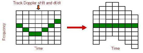
All three methods are based on summing measures of strain power from many SFTs that have been created from 30-minute intervals of calibrated strain data. Each method also corrects explicitly for sky-position dependent Doppler modulations of the apparent source frequency due to the Earth’s rotation and its orbital motion around the SSB, and the frequency’s time derivative, intrinsic to the source (see Fig. 2). This requires a search in a four-dimensional parameter space; a template in the space refers to a set of values: . The third method, PowerFlux, also searches explicitly over polarization angle, so that .
All three methods search for initial frequency in the range – Hz with a uniform grid spacing equal to the size of an SFT frequency bin,
| (11) |
where is the time-baseline of each SFT. The range of is determined by the noise curves of the interferometers, likely detectable source frequencies palomba, and limitations due to the increasing computational cost at high frequencies.
The range of values searched is , for the StackSlide and PowerFlux methods and , for the Hough method. The ranges of are determined by the computational cost, as well as by the low probability of finding an object with higher than the values searched—in other words, the ranges of are narrow enough to complete the search in a reasonable amount of time, yet wide enough to include likely signals. All known isolated pulsars spin down more slowly than the two values of used here, and as seen in the results section, the ellipticity required for higher is improbably high for a source losing rotational energy primarily via gravitational radiation at low frequencies. A small number of isolated pulsars in globular clusters exhibit slight spin-up, believed to arise from acceleration in the Earth’s direction; such spin-up values have magnitudes small enough to be detectable with the zero-spin-down templates used in these searches, given a strong enough signal. The parameter ranges correspond to a minimum spin-down timescale (the gravitational-wave spin-down age) of 40 years for a source emitting at 50 Hz and 800 years for a source at 1000 Hz. Since for known pulsars ATNF this characteristic timescale is at least hundreds of years for frequencies on the low end of our range and tens of millions of years for frequencies on the high end, we see again that the ranges of are wide enough to include sources from this population.
As discussed in our previous reports S2HoughPaper; S2FstatPaper, the number of sky points that must be searched grows quadratically with the frequency , ranging here from about five thousand at 50 Hz to about two million at 1000 Hz. All three methods use nearly isotropic grids which cover the entire sky. The PowerFlux search also divides the sky into regions according to susceptibility to stationary instrumental line artifacts. Sky grid and spin-down spacings and other details are provided below.
IV.1.2 Upper limits
While the parameter space searched is similar for the three methods, there are important differences in the way upper limits are set. StackSlide and Hough both set population-based frequentist limits on by carrying out Monte Carlo simulations of a random population of pulsar sources distributed uniformly over the sky and with isotropically distributed spin-axes. PowerFlux sets strict frequentist limits on circular and linear polarization amplitudes and , which correspond to limits on most and least favorable pulsar inclinations, respectively. The limits are placed separately on tiny patches of the sky, with the highest strain upper limits presented here. In this context “strict” means that, regardless of its polarization angle or inclination angle , regardless of its sky location (within fiducial regions discussed below), and regardless of its frequency value and spin-down within the frequency and spin-down step sizes of the search template, an isolated pulsar of true strain amplitude , would have yielded a higher measured amplitude than what we measure, in at least 95% of independent observations. The circular polarization limits apply only to the most favorable inclinations (, ), regardless of sky location and regardless of frequency and spin-down, as above.
Due to these different upper limit setting methods, sharp instrumental lines are also handled differently. StackSlide and Hough carry out removal of known instrumental lines of varying widths in individual SFTs. The measured powers in those bins are replaced with random noise generated to mimic the noise observed in neighboring bins. This line cleaning technique can lead to a true signal being missed because its apparent frequency may coincide with an instrumental line for a large number of SFTs. However, population-averaged upper limits are determined self-consistently to include loss of detection efficiency due to line removal, by using Monte Carlo simulations.
Since its limits are intended to be strict, that is, valid for any source inclination and for any source location within its fiducial area, PowerFlux must handle instrumental lines differently. Single-bin lines are flagged during data preparation so that when searching for a particular source an individual SFT bin power is ignored when it coincides with the source’s apparent frequency. If more than 80% of otherwise eligible bins are excluded for this reason, no attempt is made to set a limit on strain power from that source. In practice, however, the 80% cutoff is not used because we have found that all such sources lie in certain unfavorable regions of the sky, which we call “skybands” and which we exclude when setting upper limits. These skybands depend on source frequency and its derivative, as described in Sec. V.4.4.
IV.1.3 Data Preparation
Other differences among the methods concern the data windowing and filtering used in computing Fourier transforms and concern the noise estimation. StackSlide and Hough apply high pass filters to the data above , in addition to the filter used to produce the calibrated data stream, and use Tukey windowing. PowerFlux applies no additional filtering and uses Hann windowing with 50% overlap between adjacent SFT’s. StackSlide and Hough use median-based noise floor tracking mohanty02b; mohanty02a; badri. In contrast, Powerflux uses a time-frequency decomposition. Both of these noise estimation methods are described in Sec. V.
The raw, uncalibrated data channels containing the strain measurements from the three interferometers are converted to a calibrated “” data stream, following the procedure described in hoftpaper, using calibration reference functions described in S4CalibrationNote. SFTs are generated directly from the calibrated data stream, using 30-minute intervals of data for which the interferometer is operating in what is known as science-mode. The choice of 30 minutes is a tradeoff between intrinsic sensitivity, which increases with SFT length, and robustness against frequency drift during the SFT interval due to the Earth’s motion, source spin-down, and non-stationarity of the data S2HoughPaper. The requirement that each SFT contain contiguous data at nominal sensitivity introduces duty factor loss from edge effects, especially for the Livingston interferometer (20%) which had typically shorter contiguous-data stretches. In the end, the StackSlide and Hough searches used 1004 SFTs from H1 and 899 from L1, the two interferometers with the best broadband sensitivty. For PowerFlux, the corresponding numbers of overlapped SFTs were 1925 and 1628. The Hough search also used 1063 H2 SFTs. In each case, modest requirements were placed on data quality to avoid short periods with known electronic saturations, unmonitored calibration strengths, and the periods immediately preceding loss of optical cavity resonance.
IV.2 Definitions And Notation
Let be the number of SFTs, the time-baseline of each SFT, and the number of uniformly spaced data points in the time domain from which the SFT is constructed. If the time series is denoted by (), then our convention for the discrete Fourier transform is
| (12) |
where , and . For , the frequency index corresponds to a physical frequency of .
In each method, the “power” (in units of spectral density) associated with frequency bin and SFT is taken to be
| (13) |
It proves convenient to define a normalized power by
| (14) |
The quantity is the single-sided power spectral density of the detector noise at frequency , the estimation of which is described below. Furthermore, a threshold, , can be used to define a binary count by hough04:
| (15) |
| Quantity | Description |
|---|---|
| Power for SFT & template | |
| Normalized power for SFT & template | |
| Binary count for SFT & template | |
| Power spect. noise density for SFT & template | |
| at midpoint of SFT for template | |
| at midpoint of SFT for template |
When searching for a signal using template the detector antenna pattern and frequency of the signal are found at the midpoint time of the data used to generate each SFT. Frequency dependent quantities are then evaluated at a frequency index corresponding to the bin nearest this frequency. To simplify the equations in the rest of this paper we drop the frequency index and use the notation given in Table 1 to define various quantities for SFT and template .
IV.3 Basic StackSlide, Hough, and PowerFlux Formalism
We call the detection statistics used in this search the “StackSlide Power”, , the “Hough Number Count”, , and the “PowerFlux Signal Estimator”, . The basic definitions of these quantities are given below.
Here the simple StackSlide method described in StackSlideTechNote is used; the “StackSlide Power” for a given template is defined as
| (16) |
This normalization results in values of with a mean value of unity and, for Gaussian noise, a standard deviation of . Details about the value and statistics of in the presence and absence of a signal are given in Appendix B and StackSlideTechNote.
In the Hough search, instead of summing the normalized power, the final statistic used in this paper is a weighted sum of the binary counts, giving the “Hough Number Count”:
| (17) |
where the Hough weights are defined as
| (18) |
and the weight normalization is chosen according to
| (19) |
With this choice of normalization the Hough Number Count lies within the range . Thus, we take a binary count to have greater weight if the SFT has a lower noise floor and if, in the time-interval corresponding to this SFT, the beam pattern functions are larger for a particular point in the sky. Note that the sensitivity of the search is governed by the ratios of the different weights, not by the choice of overall scale. In the next section we show that these weights maximize the sensitivity, averaged over the orientation of the source. This choice of was originally derived in Palomba2005 using a different argument and is similar to that used in the PowerFlux circular polarization projection described next. More about the Hough method is given in S2HoughPaper; hough04.
The PowerFlux method takes advantage of the fact that less weight should be given to times of greater noise variance or smaller detector antenna response to a signal. Noting that power estimated from the data divided by the antenna pattern increases the variance of the data at times of small detector response, the problem reduces to finding weights that minimize the variance, or in other words that maximize the signal-to-noise ratio. The resulting PowerFlux detection statistic is PowerFluxTechNote,
| (20) |
where the PowerFlux weights are defined as
| (21) |
and where
| (22) |
As noted previously, the PowerFlux method searches using four linear polarization projections and one circular polarization projection. For the linear polarization projections, note that is evaluated at the angle , which is the same as evaluated at the angle ; for circular polarization, the value of is independent of . Finally note that the factor of in Eq. (20) makes dimensionless and is chosen to make it directly related to an estimate of the squared amplitude of the signal for the given polarization. Thus is also called in this paper the “PowerFlux Signal Estimator”. (See PowerFluxTechNote and Appendix A for further discussion.)
V Implementations and Pipelines
V.1 Running Median Noise Estimation
The implementations of the StackSlide and Hough methods described below use a “running median” to estimate the mean power and, from this estimate, the power spectral density of the noise, for every frequency bin of every SFT. PowerFlux uses a different noise decomposition method described in its implementation section below.
Note that for Gaussian noise, the single-sided power spectral density can be estimated using
| (23) |
where the angle brackets represent an ensemble average. The estimation of must guard against any biases introduced by the presence of a possible signal and also against narrow spectral disturbances. For this reason the mean, , is estimated via the median. We assume that the noise is stationary within a single SFT, but allow for non-stationarities across different SFTs. In every SFT we calculate the “running median” of for every frequency bins centered on the bin, and then estimate mohanty02b; mohanty02a; badri by dividing by the expected ratio of the median to the mean.
Note, however, that in the StackSlide search, after the estimated mean power is used to compute in the denominator of Eq. (14) these terms are summed in Eq. (16), while the Hough search applies a cutoff to obtain binary counts in Eq. (15) before summing. This results in the use of a different correction to get the mean in the StackSlide search from that used in the Hough search. For a running median using 101 frequency bins, the effective ratio of the median to mean used in the StackSlide search was (which was chosen to normalize the data so that the mean value of the StackSlide Power equals one) compared with the expected ratio for an exponential distribution of used in the Hough search (which is explained in Appendix A of S2HoughPaper). It is important to realize that the results reported here are valid independent of the factor used, since any overall constant scaling of the data does not affect the selection of outliers or the reported upper limits, which are based on Monte Carlo injections subjected to the same normalization.
V.2 The StackSlide Implementation
V.2.1 Algorithm and parameter space
The StackSlide method uses power averaging to gain sensitivity by decreasing the variance of the noise BCCS; BC00; cgk; StackSlideTechNote. Brady and Creighton BC00 first described this approach in the context of gravitational-wave detection as a part of a hierarchical search for periodic sources. Their method consists of averaging the power from a demodulated time series, but as an approximation did not include the beam pattern response of the detector. In Ref. StackSlideTechNote, a simple implementation is described that averages the normalized power given in Eq. (14). Its extension to averaging the maximum likelihood statistic (known as the -statistic) which does include the beam pattern response is mentioned in Ref. StackSlideTechNote (see also jks; hough04; S2FstatPaper), and further extensions of the StackSlide method are given in cgk.
As noted above, the simple StackSlide method given in StackSlideTechNote is used here and the detection statistic, called the “StackSlide Power”, is defined by Eq. (16). The normalization is chosen so that the mean value of is equal to and its standard deviation is for Gaussian noise alone. For simplicity, the StackSlide Power signal-to-noise ratio (in general the value of minus its mean value and then divided by the standard deviation of ) will be defined in this paper as , even for non-Gaussian noise.
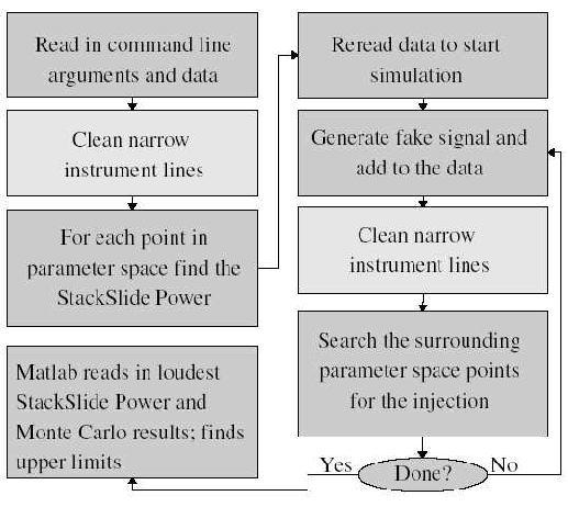
The StackSlide code, which implements the method described above, is part of the C-based LSC Algorithms Library Applications (LALapps) stored in the lscsoft CVS repository LAL. The code is run in a pipeline with options set to produce the results from a search and from Monte Carlo simulations. Parallel jobs are run on computer clusters within the LSC, in the Condor environment condor, and the final post processing steps are performed using Matlab matlab. The specific StackSlide pipeline used to find the upper limits presented in this paper is shown in Fig. 3. The first three boxes on the left side of the pipeline can also be used to output candidates for follow-up searches.
A separate search was run for each successive Hz band within Hz. The spacing in frequency used is given by Eq. (11). The spacing in was chosen as that which changes the frequency by one SFT frequency bin during the observation time , i.e., so that . For simplicity seconds days was chosen, which is greater than or equal to for each interferometer. Thus, the part of the parameter space was over-covered by choosing
| (24) |
Values of in the range were searched. This range corresponds to a search over values of , which is the same as PowerFlux used in its low-frequency search (discussed in Section. V.4).
The sky grid used is similar to that used for the all-sky search in S2FstatPaper, but with a spacing between sky-grid points appropriate for the StackSlide search. This grid is isotropic on the celestial sphere, with an angular spacing between points chosen for the - Hz band, such that the maximum change in Doppler shift from one sky grid point to the next would shift the frequency by half a bin. This is given by
| (25) |
where is the magnitude of the velocity of the detector in the SSB frame, and is the angle between and the unit-vector giving the sky-position of the source. Equations (24) and (25) are the same as Eqs. (19) and (22) in S2HoughPaper, which represent conservative choices that over-cover the parameter space. Thus, the parameter space used here corresponds to that in Ref. S2HoughPaper, adjusted to the S4 observation time, and with the exception that a stereographic projection of the sky is not used. Rather an isotropic sky grid is used like the one used in S2FstatPaper.
One difficulty is that the computational cost of the search increases quadratically with frequency, due to the increasing number of points on the sky grid. To reduce the computational time, the sky grid spacing given in Eq. (25) was increased by a factor of above Hz. This represents a savings of a factor of in computational cost. It was shown through a series of simulations, comparing the upper limits in various frequency bands with and without the factor of 5 increase in grid spacing, that this changes the upper limits on average by less than than , with a standard deviation of . Thus, this factor of increase was used to allow the searches in the Hz band to complete in a reasonable amount of time.
It is not surprising that the sky grid spacing can be increased, for at least three reasons. First, the value for given in Eq. (25) applies to only a small annular region on the sky, and is smaller than the average change. Second, only the net change in Doppler shift during the observation time is important, which is less than the maximum Doppler shift due to the Earth’s orbital motion during a one month run. (If the Doppler shift were constant during the entire observation time, one would not need to search sky positions even if the Doppler shift varied across the sky. A source frequency would be shifted by a constant amount during the observation, and would be detected, albeit in a frequency bin different from that at the SSB.) Third, because of correlations on the sky, one can detect a signal with negligible loss of SNR much farther from its sky location than the spacing above suggests.
V.2.2 Line cleaning


| IFO | Num. | Description | ||||
|---|---|---|---|---|---|---|
| Hz | Hz | Hz | Hz | |||
| H1 | 46.7 | — | 1 | 0.0 | 0.0 | Cal. Line |
| H1 | 393.1 | — | 1 | 0.0 | 0.0 | Cal. Line |
| H1 | 973.3 | — | 1 | 0.0 | 0.0 | Cal. Line |
| H1 | 1144.3 | — | 1 | 0.0 | 0.0 | Cal. Line |
| H1 | 0.0 | 1.0 | 1500 | 0.0006 | 0.0006 | 1 Hz Comb |
| L1 | 54.7 | — | 1 | 0.0 | 0.0 | Cal. Line |
| L1 | 396.7 | — | 1 | 0.0 | 0.0 | Cal. Line |
| L1 | 1151.5 | — | 1 | 0.0 | 0.0 | Cal. Line |
| L1 | 0.0 | 1.0 | 1500 | 0.0006 | 0.0006 | 1 Hz Comb |
Coherent instrumental lines exist in the data which can mimic a continuous gravitational-wave signal for parameter space points that correspond to little Doppler modulation. Very narrow instrumental lines are removed (“cleaned”) from the data. In the StackSlide search, a line is considered “narrow” if its full width is less than of the Hz band, or less than Hz. The line must also have been identified a priori as a known instrument artifact. Known lines with less than this width were cleaned by replacing the contents of bins corresponding to lines with random values generated by using the running median to find the mean power using 101 bins from either side of the lines. This method is also used to estimate the noise, as described in Section V.1.
It was found when characterizing the data that a comb of narrow Hz harmonics existed in the H1 and L1 data, as shown in Fig. 4. Table 2 shows the lines cleaned during the StackSlide search. As the table shows, only this comb of narrow Hz harmonics and injected lines used for calibration were removed. As an example of the cleaning process, Fig. 5 shows the amplitude spectral density estimated from SFTs before and after line cleaning, for the band with the Hz line at Hz.
| Excluded Bands | Description |
|---|---|
| Hz | |
| Power lines | |
| to | Power line harmonics |
| Violin modes | |
| Violin mode harmonics | |
| Violin mode harmonics |
The cleaning of very narrow lines has a negligible effect on the efficiency to detect signals. Very broad lines, on the other hand, cannot be handled in this way. Bands with very broad lines were searched without any line cleaning. There were also a number of highly disturbed bands, dominated either by the harmonics of Hz power lines or by the violin modes of the suspended optics, that were excluded from the StackSlide results. (Violin modes refer to resonant excitations of the steel wires that support the interferometer mirrors.) These are shown in Table 3. While these bands can be covered by adjusting the parameters used to find outliers and set upper limits, we will wait for future runs to do this.
V.2.3 Upper limits method
After the lines are cleaned, the powers in the SFTs are normalized and the parameter space searched, with each template producing a value of the StackSlide Power, defined in Eq. (16). For this paper, only the “loudest” StackSlide Power is kept, resulting in a value for each Hz band, and these are used to set upper limits on the gravitational-wave amplitude, . (The loudest coincident outliers are also identified, but none survive as candidates after follow-up studies described in Sec. VII.1.1.) The upper limits are found by a series of Monte Carlo simulations, in which signals are injected in software with a fixed value for , but with otherwise randomly chosen parameters, and the parameter space points that surround the injection are searched. The number of times the loudest StackSlide Power found during the Monte Carlo simulations is greater than or equal to is recorded, and this is repeated for a series of values. The confidence upper limit is defined to be the value of that results in a detected StackSlide Power greater than or equal to of the time. As shown in Fig. 3, the line cleaning described above is done after each injection is added to the input data, which folds any loss of detection efficiency due to line cleaning into the upper limits self-consistently.

Figure 6 shows the measured confidence versus for an example frequency band. The upper limit finding process involves first making an initial guess of its value, then refining this guess using a single set of injections to find an estimate of the upper limit, and finally using this estimate to run several sets of injections to find the final value of the upper limit. These steps are now described in detail.
To start the upper limit finding process, first an initial guess, , is used as the gravitational-wave amplitude. The initial guess need not be near the sought-after upper limit, just sufficiently large, as explained below. A single set of injections is done (specifically was used) with random sky positions and isotropically distributed spin axes, but all with amplitude . The output list of StackSlide Powers from this set of injections is sorted in ascending order and the ’th (specifically for the th) smallest value of the StackSlide Power is found, which we call , Note that the goal is to find the value of that makes , so that of the output powers are greater than the maximum power found during the search. This is what we call the confidence upper limit. Of course, in general will not equal unless our first guess was very lucky. However, as per the discussion concerning Eq. (61), is proportional to (i.e, removing the mean value due to noise leaves on average the power due to the presence of a signal). Thus, an estimate of the confidence upper limits is given by the following rescaling of ,
| (26) |
Thus an estimated upper limit, , is found from a single set of injections with amplitude ; the only requirement is that is chosen loud enough to make .
It is found that using Eq. (26) results in a estimate of the upper limit that is typically within of the final value. For example, the estimated upper limit found in this way is indicated by the circled point in Fig. 6. The value of then becomes the first value for in a series of Monte Carlo simulations, each with injections, which use this value and neighboring values, measuring the confidence each time. The Matlab matlab polyfit and polyval functions are then used to find the best-fit straight line to determine the value of corresponding to confidence and to estimate the uncertainties in the results. This is the final step of the pipeline shown in Fig. 3.
V.3 The Hough Transform Implementation
V.3.1 Description of Algorithm
The Hough transform is a general method for pattern recognition, invented originally to analyze bubble chamber pictures from CERN hough1; hough2; it has found many applications in the analysis of digital images ik. This method has already been used to analyze data from the second science run (S2) of the LIGO detectors S2HoughPaper and a detailed description can be found in hough04. Here we present only a brief description, emphasizing the differences between the previous S2 search and the S4 search described here.
The Hough search uses a weighted sum of the binary counts as its final statistic, as given by Eqs. (15) and (19). In the standard Hough search as presented in hough04; S2HoughPaper, the weights are all set to unity. The weighted Hough transform was originally discussed in Palomba2005. The software for performing the Hough transform has been adapted to use arbitrary weights without any significant loss in computational efficiency. Furthermore, the robustness of the Hough transform method in the presence of strong transient disturbances is not compromised by using weights because each SFT contributes at most (which is of order unity) to the final number count.
The following statements can be proven using the methods of hough04. The mean number count in the absence of a signal is , where is the number of SFTs and is the probability that the normalized power, of a given frequency bin and SFT defined by Eq. (14), exceeds a threshold , i.e., is the probability that a frequency bin is selected in the absence of a signal. For unity weighting, the standard deviation is simply . However, with more general weighting, it can be shown that is given by
| (27) |
where . A threshold on the number count corresponding to a false alarm rate is given by
| (28) |
Therefore depends on the weights of the corresponding template . In this case, the natural detection statistic is not the “Hough Number Count” , but the significance of a number count, defined by
| (29) |
where and are the expected mean and standard deviation for pure noise. Values of can be compared directly across different templates characterized by differing weight distributions.
The threshold (c.f. Eq. 15) is selected to give the minimum false dismissal probability for a given false alarm rate. In S2HoughPaper it was shown that the optimal choice for is which correspond to a peak selection probability . It can be shown that the optimal choice is unchanged by the weights and hence is used once more badrisintes.
Consider a population of sources located at a given point in the sky, but having uniformly distributed spin axis directions. For a template that is perfectly matched in frequency, spin-down, and sky-position, and given the optimal peak selection threshold, it can be shown badrisintes that the weakest signal that can cross the threshold with a false dismissal probability has an amplitude
| (30) |
where
| (31) | |||||
| (32) |
As before, and are the values of the beam pattern functions at the mid-point of the SFT. To derive (30) we have assumed that the number of SFTs is sufficiently large and that the signal is weak hough04.
From (30) it is clear that the scaling of the weights does not matter; leaves unchanged for any constant . More importantly, it is also clear that the sensitivity is best, i.e. is minimum, when is maximum:
| (33) |
This result is equivalent to Eq. (18).
In addition to improving sensitivity in single-interferometer analysis, the weighted Hough method allows automatic optimal combination of Hough counts from multiple interferometers of differing senstivities.

Ideally, to obtain the maximum increase in sensitivity, we should calculate the weights for each sky-location separately. In practice, we break up the sky into smaller patches and calculate one weight for each sky-patch center. The gain from using the weights will be reduced if the sky patches are too large. From equation (32), it is clear that the dependence of the weights on the sky-position is only through the beam pattern functions. Therefore, the sky patch size is determined by the typical angular scale over which and vary; thus for a spherical detector using the beam pattern weights would not gain us any sensitivity. For the LIGO interferometers, we have investigated this issue with Monte-Carlo simulations using random Gaussian noise. Signals are injected in this noise corresponding to the H1 interferometer at a sky-location , while the weights are calculated at a mismatched sky-position . The significance values are compared with the significance when no weights are used. An example of such a study is shown in Fig. 7. Here, we have injected a signal at , , zero spin-down, , and a signal to noise ratio corresponding approximately to a - level without weights. The figure shows a gain of at , decreasing to zero at rad. We get qualitatively similar results for other sky-locations, independent of frequency and other parameters. There is an additional gain due to the non-stationarity of the noise itself, which depends, however, on the quality of the data. In practice, we have chosen to break the sky up into 92 rectangular patches in which the average sky patch size is about rad wide, corresponding to a maximum sky position mismatch of rad in Fig. 7.
V.3.2 The Hough Pipeline
The Hough analysis pipeline for the search and for setting upper limits follows roughly the same scheme as in S2HoughPaper. In this section we present a short description of the pipeline, mostly emphasizing the differences from S2HoughPaper and from the StackSlide and PowerFlux searches. As discussed in the previous subsection, the key differences from the S2 analysis S2HoughPaper are (i) using the beam-pattern and noise weights, and (ii) using SFTs from multiple interferometers.
The total frequency range analyzed is 50-1000 Hz, with a resolution as in (11). The resolution in is given in (24), and the reference time for defining the spin-down is the start-time of the observation. However, unlike StackSlide and PowerFlux, the Hough search is carried out over only 11 values of , including zero, in the range [, ]. This choice is driven by the technical design of the current implementation, which uses look-up-tables and partial Hough maps as in S2HoughPaper. This implementation of the Hough algorithm is efficient when analyzing all resolvable points in , as given in (24), but this approach is incompatible with the larger step sizes used in the other search methods, which permit those searches to search a larger range for comparable computational cost.
The sky resolution is similar to that used by the StackSlide method for as given by (25). At frequencies higher than this, the StackSlide sky-resolution is 5 times coarser, thus the Hough search is analyzing about 25 more templates at a given frequency and spin-down value. In each of the 92 sky patches, by means of the stereographic projection, the sky patch is mapped to a two dimensional plane with a uniform grid of that resolution . Sky Patches slightly overlap to avoid gaps among them (see S2HoughPaper for further details).


Figure 8 shows examples of histograms of the number counts in two particular sky patches for the H1 detector in the 150-151 Hz band. In all the bands free of instrumental disturbances, the Hough number count distributions follows the expected theoretical distribution, which can be approximated by a Gaussian distribution. Since the number of SFTs for H1 is 1004, the corresponding mean and the standard deviation is given by Eq. (27). The standard deviation is computed from the weights and varies among different sky patches because of varying antenna pattern functions.
| IFO | Description | |||||
|---|---|---|---|---|---|---|
| Hz | Hz | Hz | Hz | |||
| H1 | 392.365 | — | 1 | 0.01 | 0.01 | Cal. SideBand |
| H1 | 393.835 | — | 1 | 0.01 | 0.01 | Cal. SideBand |
| H2 | 54.1 | — | 1 | 0.0 | 0.0 | Cal. Line |
| H2 | 407.3 | — | 1 | 0.0 | 0.0 | Cal. Line |
| H2 | 1159.7 | — | 1 | 0.0 | 0.0 | Cal. Line |
| H2 | 110.934 | 36.9787 | 4 | 0.02 | 0.02 | 37 Hz Oscillator |
| L1 | 154.6328 | 8.1386 | 110 | 0.01 | 0.01 | 8.14 Hz Comb |
| L1 | 0.0 | 36.8725 | 50 | 0.02 | 0.02 | 37 Hz Oscillator (*) |
The upper limits on are derived from the loudest event, registered over the entire sky and spin-down range in each Hz band, not from the highest number count. As for the StackSlide method, we use a frequentist method, where upper limits refer to a hypothetical population of isolated spinning neutron stars which are uniformly distributed in the sky and have a spin-down rate uniformly distributed in the range [, ]. We also assume uniform distributions for the parameters , , and . The strategy for calculating the 95 upper limits is roughly the same scheme as in S2HoughPaper, except for the treatment of narrow instrumental lines.
Known spectral disturbances are removed from the SFTs in the same way as for the StackSlide search. The known spectral lines are, of course, also consistently removed after each signal injection when performing the Monte-Carlo simulations to obtain the upper limits.
The narrow instrumental lines “cleaned” from the SFT data are the same ones cleaned during the StackSlide search shown in Table 2, together with ones listed in Table 4. The additional lines listed in Table 4 are cleaned to prevent large artifacts in one instrument from increasing the false alarm rate of the Hough multi-interferometer search. Note that the L1 36.8725 Hz comb was eliminated mid-way through the S4 run by replacing a synthesized radio frequency oscillator for phase modulation with a crystal oscillator, and these lines were not removed in the Hough L1 single-interferometer analysis.
No frequency bands have been excluded from the Hough search, although the upper limits reported on the bands shown in Table 3, that are dominated by 60 Hz power line harmonics or violin modes of the suspended optics, did not always give satisfactory convergence to an upper limit. In a few of these very noisy bands, upper limits were set by extrapolation, instead of interpolation, of the Monte-Carlo simulations. Therefore the results reported on those bands have larger error bars. No parameter tuning was performed on these disturbed bands to improve the upper limits.
V.4 The Powerflux Implementation
The PowerFlux method is a variant on the StackSlide method in which the contributions from each SFT are weighted by the inverse square of the average spectral power density in each band and weighted according to the antenna pattern sensitivity of the interferometer for each point searched on the sky. This weighting scheme has two advantages: 1) variance on the signal strength estimator is minimized, improving signal-to-noise ratio; and 2) the estimator is itself a direct measure of source strain power, allowing direct parameter estimation and dramatically reducing dependence on Monte Carlo simulations. Details of software usage and algorithms can be found in a technical document PowerFluxTechNote. Figure 9 shows a flow chart of the algorithm, discussed in detail below.
V.4.1 Noise decomposition
Noise estimation is carried out through a time/frequency noise decomposition procedure in which the dominant variations are factorized within each nominal 0.25 Hz band as a product of a spectral variation and a time variation across the data run. Specifically, for each 0.25 Hz band, a matrix of logarithms of power measurements across the mHz SFT bins and across the SFT’s of the run is created. Two vectors, denoted TMedians and FMedians, are initially set to zero and then iteratively updated according to the following algorithm:
- 1.
For each SFT (row in matrix), the median value (logarithm of power) is computed and then added to the corresponding element of TMedians while subtracted from each matrix element in that row.
- 2.
For each frequency bin (column in matrix), the median value is computed and then added to the corresponding FMedians element, while subtracted from each matrix element in that column.
- 3.
The procedure repeats from step 1 until all medians computed in steps 1 and 2 are zero (or negligible).
The above algorithm typically converges quickly. The size of the frequency band treated increases with central frequency, as neighboring bins are included to allow for maximum and minimum Doppler shifts to be searched in the next step.
For stationary, Gaussian noise and for noise that follows the above assumptions of underlying factorized frequency and time dependence, the expected distribution of residual matrix values can be found from simulation. Figure 10 shows a sample expected residual power distribution following noise decomposition for simulated stationary, Gaussian data, along with a sample residual power distribution from the S4 data (0.25-Hz band of H1 near 575 Hz, in this case) following noise decomposition. The agreement in shape between these two distributions is very good and is typical of the S4 data, despite sometimes large variations in the corresponding TMedians and FMedians vectors, and despite, in this case, the presence of a moderately strong simulated pulsar signal (Pulsar2 in Table 5).
The residuals are examined for outliers. If the largest residual value is found to lie above a threshold of 1.5, that corresponding 0.25 Hz band is flagged as containing a “wandering line” because a strong but drifting instrumental line can lead to such outliers. The value 1.5 is determined empirically from Gaussian simulations. An extremely strong pulsar could also be flagged in this way, and indeed the strongest injected pulsars are labelled as wandering lines. Hence in the search, the wandering lines are followed up, but no upper limits are quoted here for the affected bands.

V.4.2 Line flagging
Sharp instrumental lines can prevent accurate noise estimation for pulsars that have detected frequencies in the same mHz bin as the line. In addition, strong lines tend to degrade achievable sensitivity by adding excess apparent power in an affected search. In early LIGO science runs, including the S4 run, there have been sharp instrumental lines at multiples of 1 Hz or 0.25 Hz, arising from artifacts in the data acquisition electronics.
To mitigate the most severe of these effects, the PowerFlux algorithm performs a simple line detection and flagging algorithm. For each 0.25 Hz band, the detected summed powers are ranked and an estimated Gaussian sigma computed from the difference in the 50% and 94% quantiles. Any bins with power greater than 5.0 are marked for ignoring in subsequent processing. Specifically, when carrying out a search for a pulsar of a nominal true frequency, its contribution to the signal estimator is ignored when the detected frequency would lie in the same mHz bin as a detected line. As discussed below, for certain frequencies, spin-downs and points in the sky, the fraction of time a putative pulsar has a detected frequency in a bin containing an instrumental line can be quite large, requiring care. The deliberate ignoring of contributing bins affected by sharp instrumental lines does not lead to a bias in resulting limits, but it does degrade sensitivity, from loss of data. In any 0.25 Hz band, no more than five bins may be flagged as lines. Any band with more than five line candidates is examined manually.
V.4.3 Signal estimator
Once the noise decomposition is complete, with estimates of the spectral noise density for each SFT, the PowerFlux algorithm computes a weighted sum of the strain powers, where the weighting takes into account the underlying time and spectral variation contained in TMedians and FMedians and the antenna pattern sensitivity for an assumed sky location and incident wave polarization. Specifically, for an assumed polarization angle and sky location, the following quantity is defined for each bin of each SFT :
| (34) |
where is the -dependent antenna pattern for the sky location, defined in Eq. (22). (See also Appendix A.)
As in Sec. IV.2, to simplify the notation we define as the value of for SFT and a given template .
For each individual SFT bin power measurement , one expects an underlying exponential distribution, with a standard deviation equal to the mean, a statement that holds too for . To minimize the variance of a signal estimator based on a sum of these powers, each contribution is weighted by the inverse of the expected variance of the contribution. Specifically, we compute the following signal estimator:
| (35) | |||||
| (36) |
where and are the expected uncorrected and antenna-corrected powers of SFT averaged over frequency. Since the antenna factor is constant in this average, . Furthermore, is a estimate of the power spectral density of the noise. The replacement gives Eq. (20).
Note that for an SFT with low antenna pattern sensitivity , the signal estimator receives a small contribution. Similarly, SFT’s for which ambient noise is high receive small contributions. Because computational time in the search grows linearly with the number of SFT’s and because of large time variations in noise, it proves efficient to ignore SFT’s with sky-dependent and polarization-dependent effective noise higher than a cutoff value. The cutoff procedure saves significant computing time, with negligible effect on search performance.
Specifically, the cutoff is computed as follows. Let be the ordered estimated standard deviations in noise, taken to be the ordered means of , where is the number of frequency bins used in the search template. Define to be the index for which the quantity is minimized. Only SFT’s for which are used for signal estimation. In words, defines the last SFT that improves rather than degrades signal estimator variance in an unweighted mean. For the weighted mean used here, the effective noise contributions are allowed to be as high as twice the value found for . The choice of is determined empirically.
The PowerFlux search sets strict, frequentist, all-sky 95% confidence-level upper limits on the flux of gravitational radiation bathing the Earth. To be conservative in the strict limits, numerical corrections to the signal estimator are applied: 1) a factor of for maximum linear polarization mismatch, based on twice the maximum half-angle of mismatch (see Appendix A) and 2) a factor of for bin-centered signal power loss due to Hann windowing (applied during SFT generation); and 3) a factor of for drift of detected signal frequency across the width of the mHz bins used in the SFT’s. Note that the use of rectangular windowing would eliminate the need for correction 2) above, but would require a larger correction of for 3)
Antenna pattern and noise weighting in the PowerFlux method allows weaker sources to be detected in certain regions of the sky, where run-averaged antenna patterns discriminate in declination and diurnal noise variations discriminate in right ascension. Figure 11 illustrates the resulting variation in effective noise across the sky for a 0.25-Hz H1 band near 575 Hz for the circular polarization projection. By separately examining SNR, one may hope to detect a signal in a sensitive region of the sky with a strain significantly lower than suggested by the strict worst-case all-sky frequentist limits presented here, as discussed below in section VI.4. Searches are carried out for four linear polarizations, ranging over polarization angle from to in steps of and for (unique) circular polarization.

A useful computational savings comes from defining two different sky resolutions. A “coarse” sky gridding is used for setting the cutoff value defined above, while fine grid points are used for both frequency and amplitude demodulation. A typical ratio of number of coarse grid points to number of fine grid points used for Doppler corrections is 25.
V.4.4 Sky banding
Stationary and near-stationary instrumental spectral lines can be mistaken for a periodic source of gravitational radiation if the nominal source parameters are consistent with small variation in detected frequency during the time of observation. The variation in the frequency at the detector can be found by taking the time derivative of Eq. (9), which gives,
| (37) |
The detector’s acceleration, in this equation is dominated by the Earth’s orbital acceleration , since the diurnal part of the detector’s acceleration is small and approximately averages to zero during the observation. Thus, it should be emphasized that a single instrumental line can mimic sources with a range of slightly different frequencies and assumed different positions in the sky that lie in an annular band. For a source assumed to be zero, the center of the band is defined by a circle 90 degrees away from the direction of the average acceleration of the Earth during the run where , i.e., toward the average direction of the Sun during the run. For source spin-downs different from zero, there can be a cancellation between assumed spin-down (or spinup) that is largely cancelled by the Earth’s average acceleration, leading to a shift of the annular region of apparent Doppler stationarity toward (away from) the Sun.
A figure of merit found to be useful for discriminating regions of “good” sky from “bad” sky (apparent detected frequency is highly stationary) is the “ parameter”:
| (38) |
where is the Earth’s angular velocity vector about the solar system barycenter. The term is a measure of the Earth’s average acceleration during the run, where is taken to be the noise-weighted velocity of the H1 detector during the run. Regions of sky with small for a given and have stationary detected frequency. As discussed below in section VI.4, such regions are not only prone to high false-alarm rates, but the line flagging procedure described in section V.4.2 leads to systematically underestimated signal strength and invalid upper limits. Hence limits are presented here for only sources with greater than a threshold value denoted . The minimum acceptable value chosen for is found from software signal injections to be for the 1-month S4 run and can be understood to be
| (39) |
where is the minimum total number of mHz detection bins occupied by the source during the data run for reliable detection. In practice, we use still larger values for the H1 interferometer () and L1 interferometer () during the S4 run for the limits presented here because of a pervasive and strong comb of precise 1-Hz lines in both interferometers. These lines, caused by a GPS-second synchronized electronic disturbance and worse in L1 than in H1, lead to high false-alarm rates from that data for lower values of . For the frequency and spin-down ranges searched in this analysis, the average fractions of sky lost to the skyband veto are 15% for H1 and 26% for L1.
Figures 12-14 illustrate the variation in the fraction of sky marked as “bad” as assumed source frequency and spin-down are varied. Generally, at low frequencies, large sky regions are affected, but only for low spin-down magnitude, while at high frequencies, small sky regions are affected, but the effects are appreciable to larger spin-down magnitude. It should be noted that the annular regions of the sky affected depend upon the start time and duration of a data run. The longer the data run, the smaller is the region of sky for which Doppler stationarity is small. Future LIGO data runs of longer duration should have only small regions near the ecliptic poles for which stationary instrumental lines prove troublesome.


V.4.5 Grid-point upper limit determination
An intermediate step in the PowerFlux analysis is the setting of upper limits on signal strength for each sky-point for each mHz bin. The limits presented here for each interferometer are the highest of these intermediate limits for each 0.25-Hz band over the entire “good” sky. The intermediate limits are set under the assumption of Gaussian residuals in noise. In brief, for each mHz bin and sky-point, a Feldman-Cousins FeldmanCousins 95% confidence-level is set for an assumed normal distribution with a standard deviation determined robustly from quantiles of the entire 0.25 Hz band. The Feldman-Cousins approach provides the virtues of a well behaved upper limit even when background noise fluctuates well below its expectation value and of smooth transition between 1-sided and 2-sided limits, but in practice the highest upper limit for any 0.25 Hz band is invariably the highest measured power plus 1.96 times the estimated standard deviation on the background power for that bin, corresponding to a conventional a priori 1-sided 97.5% upper CL. A Kolmogorov-Smirnov (KS) statistic is computed to check the actual power against a Gaussian distribution for each 0.25 Hz band. Those bands that fail the KS test value of 0.07 ( 5 deviation for the S4 data sample) are flagged as “Non-Gaussian”, and no upper limits on pulsars are quoted here for those bands, although a full search is carried out. Bands subject to violin modes and harmonics of the 60 Hz power mains tend to fail the KS test because of sharp spectral slope (and sometimes because non-stationarity of sharp features leads to poor noise factorization).
Figure 15 provides an example of derived upper limits from one narrow band. The figure shows the distribution of PowerFlux strain upper limits on linear polarization amplitude for a sample 0.25 Hz band of S4 H1 data near 149 Hz. The highest upper limit found is (corresponding to a worst-case pulsar upper limit on of ). The bimodal distribution arises from different regions of the sky with intrinsically different antenna pattern sensitivities. The peak at corresponds to points near the celestial equator where the run-averaged antenna pattern sensitivity is worst.

VI Hardware Injections and Validation
| Name | (Hz) | () | (radians) | (radians) | (radians) | ||
|---|---|---|---|---|---|---|---|
| Pulsar0 | |||||||
| Pulsar1 | |||||||
| Pulsar2 | |||||||
| Pulsar3 | |||||||
| Pulsar4 | |||||||
| Pulsar5 | |||||||
| Pulsar6 | |||||||
| Pulsar7 | |||||||
| Pulsar8 | |||||||
| Pulsar9 | |||||||
| Pulsar10 | |||||||
| Pulsar11 |
All three methods discussed in this paper have undergone extensive internal testing and review. Besides individual unit tests of the software, hardware injections provided an end-to-end validation of the entire pipelines. The next subsections discuss the hardware injections, the validations of the three methods and their pipelines. The detection of the hardware injections also shows in dramatic fashion that we can detect the extremely tiny signals that the detectors were designed to find.
VI.1 Hardware injections
During a 15-day period in the S4 run, ten artificial isolated pulsar signals were injected into all three LIGO interferometers at a variety of frequencies and time derivatives of the frequency, sky locations, and strengths. Two additional artificial binary pulsar signals were injected for approximately one day. These hardware injections were implemented by modulating the interferometer mirror positions via signals sent to voice actuation coils surrounding magnets glued to the mirror edges. The injections provided an end-to-end validation of the search pipelines. Table 5 summarizes the nominal parameters used in the isolated-pulsar injections; the parameters are defined in section III.
Imperfect calibration knowledge at the time of these injections led to slightly different actual strain amplitude injections among the three LIGO interferometers. For the H1 and L1 comparisons between expected and detected signal strengths for these injections described in section VI.2, corrections must be applied for the differences from nominal amplitudes. The corrections are the ratios of the actuation function derived from final calibration to the actuation function assumed in the preliminary calibration used during the injections. For H1 this ratio was independent of the injection frequency and equal to 1.12. For L1, this ratio varied slightly with frequency, with a ratio of 1.11 for all injected pulsars except Pulsar1 (1.15) and Pulsar9 (1.18).
| H1 | L1 | ||||||||||
|---|---|---|---|---|---|---|---|---|---|---|---|
| Observed | Injected | Observed | Injected | Percent | Observed | Injected | Observed | Injected | Percent | ||
| Pulsar | SNR | SNR | Difference | SNR | SNR | Difference | |||||
| Pulsar0 | 0.27 | 0.23 | 1.006 | 1.005 | 0.1% | 0.15 | 0.13 | 1.003 | 1.003 | 0.1% | |
| Pulsar1 | 1.62 | 0.80 | 1.035 | 1.017 | 1.7% | 0.27 | 0.69 | 1.006 | 1.016 | 1.0% | |
| Pulsar2 | 8.92 | 8.67 | 1.179 | 1.175 | 0.4% | 8.20 | 9.34 | 1.180 | 1.203 | 1.9% | |
| Pulsar3 | 199.78 | 174.72 | 3.124 | 2.943 | 6.2% | 89.89 | 104.76 | 2.304 | 2.454 | 6.1% | |
| Pulsar4 | 2081.64 | 1872.24 | 9.607 | 9.116 | 5.4% | 1279.12 | 1425.14 | 7.895 | 8.326 | 5.2% | |
| Pulsar5 | 0.05 | 1.30 | 1.001 | 1.028 | 2.6% | 1.02 | 0.44 | 1.024 | 1.010 | 1.4% | |
| Pulsar6 | 0.17 | 2.94 | 1.004 | 1.063 | 5.5% | 2.90 | 1.36 | 1.067 | 1.032 | 3.4% | |
| Pulsar7 | 6.25 | 5.50 | 1.129 | 1.114 | 1.3% | 6.07 | 5.11 | 1.136 | 1.116 | 1.8% | |
| Pulsar8 | 98.12 | 96.21 | 2.303 | 2.285 | 0.8% | 92.77 | 103.45 | 2.334 | 2.441 | 4.4% | |
| Pulsar9 | 6.68 | 6.59 | 1.137 | 1.135 | 0.2% | 2.61 | 3.69 | 1.061 | 1.085 | 2.2% |
VI.2 StackSlide Validation
Besides individual unit tests and review of each component of the StackSlide code, we have shown that simulated signals are detected with the expected StackSlide Power, including the hardware injections listed in Table 5. Table 6 shows the observed and injected SNR, and the square root of the observed and injected StackSlide Power, . The percent difference of the latter is given, since this compares amplitudes, which are easier to compare with calibration errors. The observed values were obtained by running the StackSlide code using a template that exactly matches the injection parameters, while the injected values were calculated using the parameters in Table 5 and the equations in Appendix B. The SNR’s of Pulsar0, Pulsar1, Pulsar5, and Pulsar6 were too small to be detected, and Pulsar4 and Pulsar7 were out of the frequency band of the all-sky search. Pulsar2, Pulsar3, and Pulsar8 were detected as outliers with SNR (as discussed in Sec. VII) while Pulsar9 was not loud enough to pass this requirement. In all cases the observed StackSlide Power agrees well with that predicted, giving an end-to-end validation of the StackSlide code.

As an example of an all-sky search for a band with an injection, Fig. 16 shows the detection of Pulsar2 for a search of the H1 (top) and L1 (bottom) data, and only during the times the hardware injections were running. Later, when the entire S4 data set was analyzed Pulsar2 was still detected but with lower SNR, since this data includes times when the hardware injections were absent. Also note that, as explained in section V.4, because of strong correlations on the sky, a pulsar signal will be detected at many points that lie in an annular region in the sky that surrounds the point corresponding to the average orbital acceleration vector of the Earth, or its antipode. In fact, because of the large number of templates searched, random noise usually causes the maximum detected SNR to occur in a template other than the one which is closest to having the exact parameters of the signal. For example, for the exact template and times matching the Pulsar2 hardware injection, it was detected with SNR’s of and in H1 and L1, respectively, as given in Table 6, while the largest SNR’s shown in Fig. 16 are and . During the search of the full data set (including times when Pulsar2 was off) it was detected with SNR and in H1 and L1, respectively.
VI.3 Hough Validation


| Pulsar | Detector | range | Significance | ||
|---|---|---|---|---|---|
| (Hz) | (Hz) | ||||
| Pulsar2 | Multi-IFO | 575.15-575.18 | 575.1689 | 15.1195 | |
| H1 | 575.15-575.18 | 575.1667 | 11.1730 | ||
| L1 | 575.15-575.18 | 575.1650 | 9.7635 | ||
| Pulsar3 | Multi-IFO | 108.855-108.86 | 108.8572 | 39.1000 | |
| H1 | 108.855-108.86 | 108.8572 | 32.2274 | ||
| L1 | 108.855-108.86 | 108.8589 | 19.2267 | ||
| Pulsar8 | Multi-IFO | 193.932-193.945 | 193.9411 | 39.2865 | |
| H1 | 193.932-193.945 | 193.9394 | 27.9008 | ||
| L1 | 193.932-193.945 | 193.9400 | 23.8270 | ||
| Pulsar9 | Multi-IFO | 763.83-763.87 | 763.8511 | 8.3159 | |
| H1 | 763.83-763.87 | 763.8556 | 6.1268 | ||
| L1 | - | - | 5.4559 |
Using the Hough search code, four hardware-injected signals have been clearly detected by analyzing the data from the interval when the injections took place. These correspond to Pulsar2, Pulsar3, Pulsar8 and Pulsar9. For each of these injected signals, a small-area search ( rad rad) was performed, using a step size on the spin-down parameter of . Given the large spin-down value of Pulsar8 (), we have used 23 values of the spin-down spanning the range [, ] to search for this pulsar. Because of its large amplitude, Pulsar8 can be detected even with a large mismatch in the spin-down value, although at the cost of lower SNR.
Figure 17 shows the significance maximized over different sky locations and spin-down values for the different frequencies. These four hardware injected pulsars have been clearly detected, with the exception of Pulsar9 in the L1 data. Pulsar9 is marginally visible using the H1 data alone, with a maximum significance of 6.13, but when we combine the data from the three interferometers, the significance increases up to 8.32. Details are given in Table 7, including the frequency range of the detected signal, the frequency at which the maximum significance is obtained and its significance value.
Figure 18 shows the Hough significance maps for the multi-interferometer case. The maps displayed correspond either to the frequency and spin-down values nearest to the injected ones, or to those in which the maximum significance was observed. The location of the injected pulsars correspond to the center of each map. Note that the true spin-down value of Pulsar8, , lies between the parameter values and of the nearest templates used.
VI.4 PowerFlux validation
| Detected (Hz) | upper limit | Det. polarization | Detected SNR | |||||||
|---|---|---|---|---|---|---|---|---|---|---|
| Pulsar | (Hz) | H1 | L1 | True | H1 | L1 | H1 | L1 | H1 | L1 |
| Pulsar2 | 575.164 | 575.161 | 575.164 | circular | circular | 16.59 | 15.33 | |||
| Pulsar3 | 108.857 | 108.858 | 108.858 | circular | linear | 328.59 | 209.99 | |||
| Pulsar4 | 1402.110 | 1402.111 | 1402.113 | linear | circular | 2765.71 | 1651.82 | |||
| Pulsar7 | 1220.933 | 1220.933 | – | circular | – | 8.89 | – | |||
| Pulsar8 | 193.950 | 193.951 | 193.948 | linear | circular | 289.11 | 292.13 | |||
| Pulsar9 | 763.847 | 763.849 | – | circular | – | 8.18 | – | |||
Several cross checks have been performed to validate the PowerFlux search algorithm. These validations range from simple and rapid Fourier-domain “power injections” to more precise time domain software simulations, to hardware signal injections carried out during data taking.
Signal strain power injections have been carried out as part of PowerFlux algorithm development and for parameter tuning. These software injections involve superimposing calculated powers for assumed signals upon the LIGO power measurements and carrying out searches. For computational speed, when testing signal detection efficiency, only a small region of the sky around the known source direction is searched. A critical issue is whether the strict frequentist limits set by the algorithm are sufficiently conservative to avoid undercoverage of the intended frequentist confidence band. We present here a set of figures that confirm overcoverage applies. Figure 19 shows the difference (“excess”) between the Feldman-Cousins 95% confidence-level upper limit (conventional 97.5% upper limit) on strain and the injected strain for a sample of elliptic-polarization time-domain injections in the H1 interferometer for the 140.50-140.75 Hz band. Injection amplitudes were distributed logarithmically, while frequencies, spin-downs, sky locations, and orientations were distributed uniformly. One sees that there is indeed no undercoverage (every excess strain value is above zero) over the range of injection amplitudes. Figure 20 shows the same “excess” plotted vs the injected spin-down value, where the search assumes a spin-down value of zero, and where the sample includes injections with actual spin-down values more than a step size away from the the assumed value for the search template. As one can see, in this frequency range, a spin-down stepsize of is safe (true spin-down no more away from the assumed search value). Figure 21 shows the “excess” plotted vs the parameter that discriminates between sky regions of low and high Doppler stationarity. As shown, a value of is safe for these injections. For this search we have chosen 51 spin-down steps of for 50-225 Hz and 11 steps of for 200-1000 Hz.


More computationally intensive full time-domain signal injections were also carried out and the results found to be consistent with those from power injections, within statistical errors.
In addition, the PowerFlux method was validated with the hardware signal injections summarized in Table 5. The PowerFlux algorithm was run on all 10 isolated pulsars, including two outside the 50-1000 Hz search region, and results found to agree well with expectation for the strengths of the signals and the noise levels in their bands. Table 8 shows the results of the analysis for the six pulsars for which a detection with SNR7 is obtained by PowerFlux for one or both of the 4-km interferometers. Figure 22 shows a sky map of PowerFlux polarization SNR for the 0.25 Hz band containing pulsar 2 (575.16 Hz).

VII Results
All three methods described in Sections IV and V have been applied in an all-sky search over a frequency range 50-1000 Hz. As described below, no evidence for a gravitational wave signal is observed in any of the searches, and upper limits on sources are determined. For the StackSlide and Hough methods, 95% confidence-level frequentist upper limits are placed on putative rotating neutron stars, assuming a uniform-sky and isotropic-orientation parent sample. Depending on the source location and inclination, these limits may overcover or undercover the true 95% confidence-level band. For the PowerFlux method, strict frequentist upper limits are placed on linearly and circularly polarized periodic gravitational wave sources, assuming worst-case sky location, avoiding undercoverage. The limits on linear polarization are also re-interpreted as limits on rotating neutron stars, assuming worst-case sky location and worst-case star inclination. The following subsections describe these results in detail.
VII.1 StackSlide Results
VII.1.1 Loudest powers and coincidence outliers

The StackSlide method was applied to the S4 H1 and L1 data set, as given in Sec. V.2. As described in that section, only the loudest StackSlide Power was returned from a search of the entire sky, the range of the frequency’s time derivative, Hz , and for each Hz band within Hz. The results are shown in Fig. 23.

| (Hz) | (Hz) | H1 SNR | L1 SNR | Comment | |
|---|---|---|---|---|---|
| 1 | 78.618889 | 78.618889 | 14.82 | 13.58 | Inst. Lines |
| 2 | 108.856111 | 108.856111 | 152.11 | 69.79 | HW Inj. Pulsar3 |
| 3 | 193.947778 | 193.949444 | 121.89 | 125.75 | HW Inj. Pulsar8 |
| 4 | 244.148889 | 244.157778 | 9.00 | 22.89 | Inst. Lines |
| 5 | 375.793889 | 375.806667 | 11.68 | 27.09 | HW Inj. Pulsar11 |
| 6 | 376.271111 | 376.281667 | 7.47 | 9.46 | HW Inj. Pulsar11 |
| 7 | 575.162778 | 575.153333 | 11.09 | 10.71 | HW Inj. Pulsar2 |
| 8 | 575.250000 | 575.371667 | 7.49 | 7.51 | Inst. Lines |
| 9 | 575.250000 | 575.153333 | 7.49 | 10.71 | Inst. & Pulsar2 |
| 10 | 580.682778 | 580.734444 | 7.02 | 7.19 | Inst. Lines |
| 11 | 912.307778 | 912.271111 | 7.02 | 7.37 | Inst. Lines |
| 12 | 988.919444 | 988.960556 | 9.56 | 9.75 | Inst. Lines |
| 13 | 988.919444 | 989.000000 | 9.56 | 8.12 | Inst. Lines |
| 14 | 993.356111 | 993.523333 | 7.08 | 7.12 | Inst. Lines |
Many of the StackSlide results have power greater than expected due to random chance alone (for Gaussian noise). To identify the most interesting subset of these cases, a simple coincidence test was applied: only results with an SNR greater than in both H1 and L1 and with a fractional difference in frequency, measured in the SSB, less than or equal to were identified as outliers for further follow-up. The requirement on frequency agreement comes from the worst-case scenario where a signal is detected on opposite sides of the sky with opposite Doppler shifts of and , giving a maximum fraction difference in the detected frequency at the SSB of . The results after applying this simple coincidence test are shown in Fig. 24. The outliers that passed the test are shown in Table 9.
Note that the coincidence test used on the StackSlide results is very conservative in that it only covers the worst-case frequency difference, and makes no requirement on consistency in sky position or the frequency’s time derivative. However it is meant to find only the most prominent outliers. Since an automated follow-up of possible candidates is not yet in place, the follow-up is carried out manually. This dictated using a large threshold on SNR. Also, since the false dismissal rate of the coincidence test used was not determined (though it is assumed to be essentially zero) it is not used in this paper when setting upper limits. Monte Carlo studies will be needed to find appropriate thresholds on SNR and the size of coincidence windows, so that proper false alarm and false dismissal rates can be determined; such studies will be carried out when analyzing future data sets.


Three types of qualitative follow-up tests were performed on each of the outliers in Table 9. First, using the sky position and the value of the template that gives the outlier in H1, the StackSlide Power was found using the same values for these in L1 and H2 for a frequency band around that of the outlier in H1. For a fixed sky position and , a true gravitational-wave signal should show up in all three detectors as a narrow line at nearly the same frequency (though with an SNR corresponding to half the length displacement in H2 compared with that in H1 and L1). Second, the StackSlide Power was computed for the frequency bands containing the outliers, with sliding turned off. If an instrumental line is the underlying cause of the outlier, a stronger and narrower peak will tend to show up in this case. Third, the StackSlide Power was computed for each H1 outlier template, using half (and some other fractions) of the data. This should reduce the SNR of a true signal by roughly the square root of the fractional reduction of the data, but identify transient signals, which would fail this test by showing up in certain stretches of the data with more SNR while dissappearing in other stretches. This would be true of the hardware injections which were not always on during the run, or temporary disturbances of the instrument which appear to look like signals only for limited periods of time. (The search described here was not designed to find truely transient gravitational-wave signals.)
The follow-up tests on the outliers given in Table 9 found that none is qualitatively consistent with a true gravitational-wave signal. The three loudest hardware injections of periodic gravitational waves from fake isolated sources were found (indicated as Pulsar3, Pulsar8, and Pulsar2), as well as interference from a fake source in a binary system (Pulsar11). All of the outliers due to the hardware injections show up in the H1 template as relatively narrow lines in all three detectors, for example as shown in Fig. 25. These outliers, on the other hand, fail the third test when looking at times the hardware injections were turned off. In particular, this test, along with the frequencies in Table 5, confirms the identification of outliers and as due to Pulsar11. The other hardware injections also are identified as such via their detected frequencies in Table 5 and SNRs in Table 6. In comparison, none of the other outliers qualitatively passes the first test, for example as shown in Fig. 26. The second test was less conclusive, since some of the outliers lie at points on the sky that receive little Doppler modulation, but based on the first test we conclude that the remaining outliers are only consistent with instrumental line artifacts. These results are summarized in column six of Table 9. In future searches, tests of the type used here should be studied using Monte Carlo simulations, to make them more quantitative.
VII.1.2 StackSlide upper limits

| Detector | Band (Hz) | |
|---|---|---|
| H1 | 139.50-139.75 | |
| L1 | 140.75-141.00 |
The StackSlide confidence upper limits on are shown as crosses for H1 (top) and L1 (bottom) respectively in Fig. 27, while the solid curves in this figure show the corresponding characteristic amplitudes given by Eq. (67) in Appendix B. The characteristic amplitudes were calculated using an estimate of the noise from a typical time during the run, but include bands with the power line and violin line harmonics which were excluded from the StackSlide search. The best upper limits over the entire search band are given in Table 10. The uncertainties in the upper limits and confidence due to the method used are less than or equal to and respectively; random and systematic errors from the calibration increase these uncertainties to about .
VII.2 Hough results
VII.2.1 Number Counts
For the S4 data set, there are a total of SFTs from the three interferometers, giving an expected average number count for pure noise of . The standard deviation now depends on the sky-patch according to (27). For reference, if we had chosen unit weights, the standard deviation assuming pure Gaussian noise would have been for the multi-interferometer search. To compare number counts directly across different sky-patches, we employ the significance of a number count defined in Eq. (29).
Since the three interferometers have different noise floors and duty factors, we would like to know their relative contributions to the total Hough number count, and whether any of the interferometers should be excluded from the search, or if all of them should be included. For this purpose, for the moment let us ignore the beam pattern functions and consider just the noise weighting: . The relative contribution of a particular interferometer, say , is given by the ratio
| (40) |
The numerator is a sum of the weights for the interferometer while the denominator is the sum of all the weights. This figure-of-merit incorporates both the noise level of data from an interferometer, and also its duty cycle as determined by the number of SFTs available for that interferometer. Figure 28 shows the relative contributions from H1, L1, and H2 for the duration of the S4 run. From the plot, we see that H1 clearly contributes the most. H2 contributes least at low frequencies while L1 contributes least at higher frequencies. Hence all three LIGO interferometers are included in this search. For comparison purposes and for coincidence analysis, we have also analyzed the data from H1 and L1 separately.


Figure 29 shows the result of the Hough search using data from all three LIGO interferometers, either combined in a multi-interferometer search, or just for H1 and L1 data. This figure shows the loudest significance in every Hz band, maximized over all sky-positions, frequencies and spin-downs for the three searches. Line cleaning was used as described before. In the bands in which there are no spectral disturbances the significance distribution agrees very well with the theoretical expected distribution as was shown in Fig. 8.
VII.2.2 Study of coincidence outliers
There are many outliers from the Hough search with significance values higher than expected for Gaussian noise, as shown in Fig. 29. Many of the large outliers correspond to well known instrumental artifacts described earlier, such as the power mains harmonics or the violin modes.
Note the relation between significance and false alarm which can be derived from equations (28) and (29) for Gaussian noise:
| (41) |
To identify interesting candidates, we consider only those that have a significance greater than 7 in the multi-interferometer search (the most sensitive one). This is the same threshold considered by the StackSlide and PowerFlux searches. For the Hough search, this threshold corresponds to a false alarm rate of . With this threshold, we would expect about 6 candidates in a 100 Hz band around 1 kHz for Gaussian noise, since the number of templates analyzed in a 1 Hz band around 1 kHz is about . If we would like to set a different threshold in order to select, say one event in a 1 Hz band, then we should increase the false alarm to .
In order to exclude spurious events due to instrumental noise in just one detector, we pass these candidates through a simple coincidence test in both the H1 and the L1 data. Since the single detector search is less sensitive than the multi-interferometer one, we consider events from H1 and L1 with a significance greater than 6.6, corresponding to a false alarm rate of . The numbers of templates analyzed using the H1 or L1 data are the same as for the multi-interferometer search.
| Hough significance | |||||
| Band (Hz) | Multi-IFO | H1 | L1 | Comment | |
| 1 | 78.602-78.631 | 12.466 | 12.023 | 10.953 | Inst. Lines |
| 2 | 108.850-108.875 | 29.006 | 23.528 | 16.090 | Inj. Pulsar3 |
| 3 | 130.402-130.407 | 7.146 | 6.637 | 6.989 | ? |
| 4 | 193.92-193.96 | 27.911 | 17.327 | 20.890 | Inj. Pulsar8 |
| 5 | 575.15-575.23 | 13.584 | 9.620 | 10.097 | Inj. Pulsar2 |
| 6 | 721.45-721.50 | 8.560 | 6.821 | 13.647 | L1 Inst. Lines |
| 7 | 988.80-988.95 | 7.873 | 8.322 | 7.475 | Inst. Lines |


| Detector | (Hz) | () | (rad) | (rad) | |
|---|---|---|---|---|---|
| Multi-IFO | 7.146 | 130.4028 | 0.8798 | -1.2385 | |
| H1 | 6.622 | 130.4039 | 2.1889 | 0.7797 | |
| H1 | 6.637 | 130.4050 | 2.0556 | 0.6115 | |
| L1 | 6.989 | 130.4067 | 1.1690 | -1.0104 |
The coincidence test applied first in frequency is similar to the one described for the StackSlide search, using a coincidence frequency window as broad as the size of the maximum Doppler shift expected at a given frequency. Of the initial 3800 0.25-Hz bands investigated, 276 yielded outliers in the multi-interferometer search with a significance higher than 7. Requiring those bands (or neighboring bands) to have outliers in H1 higher than 6.6, reduced by half the number of surviving bands. These remaining bands were studied in detail and, after eliminating power line harmonics and the violin modes, 27 candidates remained. Applying again the same coincidence test with the L1 data, we are left with only 7 coincidence outliers that are listed on Table 11 and displayed in Fig. 30.
Except for the third outlier, the coincidence can be attributed to instrumental lines in the detectors or to the hardware pulsar injections. Table 12 summarizes the parameters of the third coincidence candidate in the 130.40-130.41 Hz frequency band, including all the events that in any of the searches had a significance larger than 6.6. As can be seen from the Table, the events from the different data sets correspond to widely separated sky locations. Hence no detections were made in the Hough search of the S4 data.
In future searches we plan to use lower thresholds in the semi-coherent step in order to point to interesting areas in parameter space to be followed up, using a hierarchical scheme with alternating coherent and semicoherent steps. In what follows we will concentrate on setting upper limits on the amplitude in each of the 0.25 Hz bands.
VII.2.3 Upper limits


| Detector | Band (Hz) | ||
|---|---|---|---|
| H1+H2+L1 | 140.00-140.25 | ||
| H1 | 129.00-129.25 | ||
| L1 | 140.25-140.50 |
As in the previous S2 Hough search S2HoughPaper, we set a population based frequentist upper limit using Monte Carlo signal software injections. We draw attention to two important differences from that analysis:
- •
In S2HoughPaper, known spectral disturbances were handled by simply avoiding all the frequency bins which could have been affected by Doppler broadening. Thus, the loudest event was obtained by excluding such frequency bins, and the subsequent Monte Carlo simulations also did not perform any signal injections in these bins. Here we follow the same approach as used in the StackSlide search; we use the spectral line removal procedure described in section V.2.1. For consistency, the same line removal procedure is followed in the Monte Carlo simulation after every software injection.
- •
Recall that the calculation of the weights depends on the sky-patch, and the search has been carried out by breaking up the sky in 92 patches. Thus, for every randomly injected signal, we calculate the weights corresponding to the center of the corresponding sky patch. The analysis of S2HoughPaper did not use any weights and this extra step was not required.
The 95 confidence all-sky upper limit results on from the Hough search for the multi-interferometer, H1 and L1 data are shown in Fig. 31. These upper limits have been obtained by means of Monte-Carlo injections in each 0.25 Hz band in the same way as described in S2HoughPaper. The best upper limit over the entire search band corresponds to for the multi-interferometer case in the Hz band. The results are summarized in Table 13.
Let us now understand some features of the upper-limit results. First, it turns out that it is possible to accurately estimate the upper limits without extensive Monte Carlo simulations. From (30), and setting , we expect that the upper limits are:
| (42) |
Recall that contains contributions both from the sky-location-dependent antenna pattern functions and from the sky-location-independent noise floor estimates. However, since we are setting upper limits for a population uniformly distributed in the sky, we might expect that the are more important for estimating the value of . From Eq. (32) and averaging over the sky we get
| (43) |
and thus, up to a constant factor , the estimated upper limits are given by
| (44) |
The value of is calculated from Eq. (31) using the false alarm corresponding to the significance of the observed loudest event in a particular frequency band. The value of the false dismissal rate corresponds to the desired confidence level of the upper limit (in this case ). To show that such a fit is viable, Fig. 32 plots the value of the constant appearing in the above equation for every Hz frequency band, using the measured upper limits. It turns out that . The exact value of depends on the interferometer and the search performed, but it is still found to lie within this range. This scale factor is about two times worse than we would expect if we were performing a targeted (multi-interferometer with weights) search with no mismatch. This factor of two is also in very good agreement with what was reported in the S2 search S2HoughPaper.
The utility of this fit is that having determined the value of in a small frequency range, it can be extrapolated to cover the full bandwidth without performing any further Monte Carlo simulations. Figure 33 plots the ratio of the measured upper limits to the estimated values showing the accuracy of the fit. The scale factors used are 9.2 for the multi-interferometer search, 9.7 for H1 and 9.3 for L1. The scale factors have been obtained in all cases by comparing the measured upper limits by means of Monte Carlo injections to the quantity as defined in Equation (44), using the full bandwidth of the search. These estimated upper limits have an error smaller than for bands free of large instrumental disturbances.

We conclude this section by quantifying the improvement in sensitivity caused by using the weights. Figure 34 shows the comparison between the weighted and un-weighted results in the -Hz frequency range. The average improvement is in this band. It is easy to see that the improvement as compared to the unweighted Hough search will be larger if the variation of and the beam pattern functions is large across the SFTs. Since the variation in is larger in a multi-interferometer search, we expect this improvement to be much more significant in a multi-interferometer search. For the case of analyzing data from a single interferometer, for example H1, the improvement in the upper limits due to the weights turns out to be only . Also, the improvement can be increased by choosing smaller sky-patches so that the weight calculation is more optimal. In particular, if there would not be any sky mismatch in computing the weights, only due to the amplitude modulation, i.e., in the presence of Gaussian and stationary noise, we would expect an average increase of sensitivity of , and it could be up to for optimally oriented pulsars. These results have been verified experimentally by means of a set of Monte-Carlo tests badrisintes.
VII.3 PowerFlux results
VII.3.1 Single-interferometer results
The PowerFlux method has been applied to the S4 data sample in the range 50-1000 Hz. Five polarization projections are sampled for each grid point: four linear polarizations with = 0, , , ; and circular polarization. For each sky grid point in the “good sky” defined above and each of the 501 frequency bins (there is slight overlap of 0.25 Hz bands), the Feldman-Cousins FeldmanCousins 95% CL upper limit is computed, as described in section V.4.5, for each polarization projection. Worst-case upper limits on linear polarization for each grid point and frequency are taken to be the highest linear-polarization-projection strain limit divided by to correct for worst-case polarization mismatch. The highest limit for all frequency bins in the 0.25 Hz band and over all sampled sky points is taken to be the broad-sky limit for that 0.25 Hz band. Figures 35-36 show the resulting broad-sky limits on linearly polarized periodic sources from H1 and L1. Bands flagged as non-Gaussian (instrumental artifacts leading to failure of the KS test) or near 60-Hz harmonics are indicated by color. The derived upper limits for these bands are considered unreliable. Diamonds indicate bands for which wandering instrumental lines (or very strong injected signals) lead to degraded upper limits. An exceedingly strong pulsar can be identified as a wandering line, and several strong hardware-injected pulsars are marked in the figures as such.
These limits on linearly polarized radiation and the corresponding limits on circularly polarized radiation can be interpreted as worst-case and best-case limits on a triaxial-ellipsoid, non-precessing neutron star, respectively, as discussed in Appendix A. Multiplying the linear-polarization limits by a factor of two leads to the worst-case H1 limits on shown in Figs. 37–38. The circular-polarization limits require no scale correction. Note that the StackSlide and Hough H1 limits shown on the same figure apply to a uniform-sky, uniform-orientation population of pulsars.


VII.3.2 Coincidence followup of loud candidates
All outliers (SNR7, diamonds, and non-Gaussian bands) in the single-interferometer analysis are checked for coincidence between H1 and L1. In this followup, agreement is required in frequency to within 10 mHz, in spin-down to within , and in both right ascension and declination to within 0.5 radians. The only surviving candidates are associated with hardware-injected pulsars 2, 3, 4, and 8 (see Table 8), 1-Hz harmonics, violin modes, and instrumental lines in both detectors near 78.6 Hz (also seen in the StackSlide and Hough searches). The source of these lines remains unknown, but followup consistency checks described in section VII.1 rule out an astrophysical explanation.
From this coincidence analysis, we see no evidence of a strong pulsar signal in the S4 data. It should be noted, however, that the SNR threshold of 7 is relatively high. A lower threshold and a more refined algorithm for location and frequency coincidence is under development for future searches.
VIII Comparison of the Three Methods


Figures 37 and 38 show superimposed the final upper limits on from the StackSlide, Hough, and PowerFlux methods when applied to the S4 single-interferometer H1 and L1 data, respectively. As one might have expected, we see that the StackSlide and Hough population-based limits lie between the best-case and worst-case strict limits from PowerFlux. As indicated in Figs. 37–38, the Hough search sensitivity improves with the summing of powers from two or more interferometers.
To be more precise as to expectations, we have directly compared detection efficiencies of the three methods in frequency bands with different noise characteristics. As discussed above, we expect overall improved performance of Powerflux with respect to StackSlide and Hough, except possibly for frequency bands marked by extreme non-Gaussianity or non-stationarity, where the Hough integer truncation of extreme power outliers can provide more robustness. We do not consider computational efficiency, which could play an important role in deciding which algorithm to use in computationally limited hierarchical searches.


A comparison is shown in Figs. 39 and 40 among the efficiencies of the three methods for two particular 0.25 Hz bands for H1: 140.5–140.75 Hz and 357–357.25 Hz. The horizontal axis in each case is the of Monte Carlo software injections with random sky-locations, spin-downs and orientations. The noise in the two bands have qualitatively different features. The 140.5-140.75 Hz band is a typical “clean” band with Gaussian noise and no observable spectral features. As expected, Fig. 39 shows that the efficiency for the PowerFlux method is higher than that for StackSlide, while that of StackSlide is better than that for Hough. In other bands, where there are stationary spectral disturbances, we find that PowerFlux remains the most efficient method.
The noise in the band 357-357.25 Hz is non-Gaussian and displays a large transient spectral disturbance, in addition to stationary line noise at 357 Hz itself. The stationary 357 Hz line was removed during the StackSlide and Hough searches, avoided during the PowerFlux search, and handled self-consistently during Monte Carlo software injections. In this band, the Hough transform method proves to be robust against transient noise, and more sensitive than the StackSlide or PowerFlux implementations (see Fig. 39). In fact, no PowerFlux upper limit is quoted for this band because of the large non-Gaussianity detected during noise decomposition. Note that the SNR thresholds used for Stackslide, Hough and PowerFlux in Fig. 40 are set to 6.3, 5.2 and 30, respectively, to match their loudest events in this band of the data.
IX Summary, Astrophysical Reach, and Outlook
In summary, we have set upper limits on the strength of continuous-wave gravitational radiation over a range in frequencies from 50 Hz to 1000 Hz, using three different semi-coherent methods for summing of strain power from the LIGO interferometers. Upper limits have been derived using both a population-based method applicable to the entire sky and a strict method applicable to regions of the sky for which received frequencies were not stationary during the S4 data run.
The limits have been interpreted in terms of amplitudes for pulsars and in terms of linear and circular polarization amplitudes, corresponding to least favorable and most favorable pulsar inclinations, respectively. As a reminder, sets of known instrumental spectral lines have been cleaned from the data prior to setting the population-based StackSlide and Hough upper limits (Tables 2, 3, and 4), while regions of the sky (defined by cutoff values on the parameter (Equations 38 and 39) have been excluded in the strict PowerFlux upper limits. The numerical values of the upper limits can be obtained separatelyepaps.
We have reached an important milestone on the road to astrophysically interesting all-sky results: Our best upper limits on are comparable to the value of a few times at which one might optimistically expect to see the strongest signal from a previously unknown neutron star according to a generic argument originally made by Blandford (unpublished) and extended in our previous search for such objects in S2 data S2FstatPaper. The value from Blandford’s argument does not depend on the distance to the star or its ellipticity, both of which are highly uncertain.

We find the next milestone by considering the maximum distance to which a signal could be detected and the ellipticity needed to generate a signal of the required strength at that distance. Both quantities are of interest since there are theoretical limits on the ellipticity, and both quantities are functions of the gravitational-wave frequency and its derivative . Figure 41 is a contour plot of both quantities simultaneously, which we explain here in more detail. The Hough transform multi-interferometer upper limits on are used for illustration because they fall in the middle of the range of values for the different searches (see Fig. 37). The maximum distance is obtained by equating the 95% confidence upper limits on for the multiple-interferometer plot in Fig. 31 to the spin-down limit given in Eq. (7). This tacitly assumes that is entirely due to emission of gravitational radiation, which implies the ellipticity given in Eq. (8) regardless of the data and the distance to the source. If we relaxed this assumption, knowing that neutron stars spin down due to electromagnetic wave emission, relativistic particle winds, and other factors as well, the maximum distance and required ellipticity for a given and would both be reduced. The degree of reduction would, however, be highly uncertain.
We can use the combined contour plot in Fig. 41 to answer questions about the astrophysical significance of our results. Here we ask and answer several salient questions. First, what is the maximum range of the Hough transform search? The answer is obtained from looking at the top of Fig. 41: We could detect isolated pulsars to about 1 kpc, but only for a star radiating at a frequency near 100 Hz and then only if that star has an ellipticity somewhat more than , which is allowed only in the most extreme equations of state Owen:2005fn; Xu:2003xe; Mannarelli:2007bs. Second, what is the maximum range of detection for a normal neutron star? Normal neutron stars are expected to have based on theoretical predictions Ushomirsky:2000ax. By tracing the contour, we find that the maximum range is about 50 pc at the highest frequencies (1 kHz), falling with frequency to less than 2 pc below 100 Hz. Third, what is the maximum range for a recycled millisecond pulsar? Based on the observed sample ATNF, recycled pulsars usually have small values, corresponding to usually less than . Unfortunately the contour corresponds to pc at all frequencies in the LIGO band.
Figure 41 then demonstrates that we have reached a second milestone not achieved in our previous all-sky searches S2HoughPaper; S2FstatPaper: The multi-interferometer Hough transform search could have detected an object at the distance of the nearest known neutron star RX J1856.53754, which is about 110–170 pc from Earth Walter:2002uq; vanKerkwijk:2006nr. We could not have detected that particular star, since the recently observed 7 s rotation period Tiengo:2006eb puts the gravitational wave frequency well out of the LIGO band. But the top of Fig. 41 shows that we could have detected a Crab-like pulsar ( Hz, ) at that distance if gravitational radiation dominated its spin-down.
For the ongoing S5 data run, expected to finish data collection in late 2007, several refinements of these methods are under development. The StackSlide and Hough methods can be made more sensitive than PowerFlux by starting with the maximum likelihood statistic (known as the -statistic jks; hough04; S2FstatPaper) rather than SFT power. This increases the time-baseline of the coherent step in a hierarchical search, though at increased computational cost. The lower computational cost of the Hough search would be an advantage in this case. Multi-interferometer searches also increase the sensitivity, while reducing outliers (false-alarms), without having to increase greatly the size of the parameter space used, as illustrated by the Hough search in this paper. A multi-interferometer version of PowerFlux is under development, as well as hierarchical multi-interferometer searches that use the Hough and StackSlide method on the -statistic.
Thus, PowerFlux will be the primary tool used for semi-coherent searches using SFTs, while the Hough and StackSlide methods will be used in multi-interferometer hierarchical searches. Strong candidates from the PowerFlux search will be fed into the latter type of search as well. The parameter space searches described here do not take into account the correlations that exist between points in the four or five dimensional parameter space (including those on the sky). A map of the mismatch between a signal and the parameter-space templates can be used to generate a parameter-space metric to reduce further the number of points needed to conduct a search, a method under development for the hierarchical searches. Finally, the strain noise of the S5 data is lower by about a factor of 2, and the run will accumulate at least year of science mode data.
Appendix A PowerFlux polarization projection relations
The PowerFlux method uses circular and four linear polarization “projections” to increase sensitivity to different source polarizations PowerFluxPolarizationNote. The projections are necessarily imperfect because the interferometer itself is a polarimeter continually changing its orientation with respect to a source on the sky. There is “leakage” of one polarization into another’s projection. In this appendix we present the formulae used by PowerFlux to define these imperfect projections and discuss corrections one can make for leakage in followup studies of candidates.
As described in section V.4.3, the signal estimator used by PowerFlux for frequency bin and projection polarization angle is
| (45) |
where is the weight for SFT and is the antenna pattern factor for a source with polarization with respect to a major axis of polarization angle .
For a source of true polarization angle and plus / cross amplitudes and , where and , the strain amplitudes projected onto the and axes for a polarization angle are
| (46) | |||||
| (47) | |||||
where , where the SFT-dependent phase constant has been taken to be zero, for convenience, and where frequency variation of the source during each 30-minute SFT interval has been neglected. Averaging the detectable signal power over one SFT interval , one obtains approximately (neglecting antenna rotation during the half-hour interval):
| (48) | |||||
Note that for a linearly polarized source with polarization angle (so that ) and amplitude , , one obtains
| (49) |
and that for a circularly polarized source of amplitude ,
| (50) |
as expected.
For an average of powers from many SFT’s, weighted according to detector noise and antenna pattern via , the expectation value of the signal estimator depends on
| (51) | |||||
where is the expected power from noise alone, where is assumed to vanish (signal uncorrelated with noise), and where the frequency bin index is omitted for simplicity.
For a true source with parameters , , and , this expectation value can be written:
| (52) | |||||
where the correction coefficients
| (53) | |||||
| (54) |
depend implicitly on through and .
For a linearly polarized source with polarization angle , one obtains
| (55) |
and for a circularly polarized source one obtains:
| (56) |
These formulae permit corrections for polarization leakage to be applied for a hypothetical source, allowing for estimation of , , and from a sampling of polarization projection measurements. In practice, however, the calculation of the coefficients is computationally costly in an all-sky search and is disabled by default. Instead, upper limits on linearly polarized sources (worst-case pulsar inclination) are derived from the maximum limit over all four linear polarization projections, as described in section V.4.3. In followup investigations of outliers, however, these formulae permit greater discrimination of candidates, now in use for PowerFlux searches of the data from the ongoing S5 data run.
Appendix B StackSlide Power And Statistics
B.0.1 Approximate Form For The StackSlide Power
It is useful to have an analytic approximation for the StackSlide Power . For a single SFT (dropping the SFT index ) expressing the phase in a first-order Taylor expansion about the midpoint time, , of the interval used to generate an SFT, we can write
| (57) |
where and are the phase and frequency at time . Treating the values of and as constants equal to their values at time , the signal strain at discrete time is approximately,
| (58) |
where gives the start time of the SFT, and is the approximate phase at the start of the SFT (not the initial phase at the start of the observation), i.e.,
| (59) |
Using these approximations, the Discrete Fourier Transform, given by Eq. (12), of is
| (60) |
where and is usually not an integer. Equation (B.0.1) holds for and , which is true for all of the frequencies over which we search.
If the discrete time samples of the data from the detector consist of a signal plus noise the expected value of is approximated by
| (61) |
where the mean value of is and its standard deviation is due to the normalization used, and
| (62) |
is an approximate form for the square of the optimal SNR defined in Eq. (71) in reference jks averaged over SFTs (i.e., the angle brackets on represent an average over SFTs) and where for each SFT the index is the nearest integer value to . Thus, the relevant range for is to , corresponding to a frequency mismatch of to of an SFT frequency bin.
B.0.2 StackSlide Statistics
It can be seen from Eq. (16) that, for Gaussian noise in the absence of a signal, is a variable with degrees of freedom StackSlideTechNote. Thus, the quantity
| (63) |
follows the distribution:
| (64) |
When a signal is present, follows a non-central distribution with degrees of freedom and a non-centrality parameter such that
| (65) |
where the form given here is based on that given in jksIII, and is the modified Bessel function of the first kind and order .
The distribution described by Eqs. (64) and (B.0.2) can be used to find the minimum optimal signal-to-noise ratio that can be detected using the StackSlide search for fixed false alarm and false dismissal rates, for a targeted search. For a false alarm rate, a false dismissal rate, and large Eqs. (63) and (B.0.2) give (See also StackSlideTechNote), while averaging Eq. (B.0.1) independently over the source sky position, inclination angle, polarization angle, and mismatch in frequency gives (see also Eq. 5.35 in hough04 ). Equating these and solving for , the characteristic amplitude for a targeted StackSlide search with a false-alarm rate, false-dismissal rate is:
| (66) |
where is the actual duration of the data, which is shorter than the total observation time, , because gaps exist in the data for times when the detectors were not operating in science mode. Comparing this expression with Eq. 5.35 in hough04 the StackSlide characteristic amplitude given in Eq. (66) is found to be about lower than a similar estimate for the standard Hough search. Note that in this paper an improved version of the Hough method is presented. Also, in this paper an all-sky search for the loudest StackSlide Power is carried out, covering up to templates, and only the loudest StackSlide Power is returned from the search, corresponding to a false alarm rate of . Furthermore, the upper limits are found by injecting a family of signals, each of which has a StackSlide Power drawn from a different noncentral chi-squared distribution. Using the results from Sec. VII, for an all-sky StackSlide search the confidence all-sky upper limits are found empirically to be approximately given by:
| (67) |
Appendix C Acknowledgments
The authors gratefully acknowledge the support of the United States National Science Foundation for the construction and operation of the LIGO Laboratory and the Particle Physics and Astronomy Research Council of the United Kingdom, the Max-Planck-Society and the State of Niedersachsen/Germany for support of the construction and operation of the GEO600 detector. The authors also gratefully acknowledge the support of the research by these agencies and by the Australian Research Council, the Natural Sciences and Engineering Research Council of Canada, the Council of Scientific and Industrial Research of India, the Department of Science and Technology of India, the Spanish Ministerio de Educacion y Ciencia, The National Aeronautics and Space Administration, the John Simon Guggenheim Foundation, the Alexander von Humboldt Foundation, the Leverhulme Trust, the David and Lucile Packard Foundation, the Research Corporation, and the Alfred P. Sloan Foundation. This document has been assigned LIGO Laboratory document number LIGO-P060010-06-Z.
References
- (1)
- (2) A. Abramovici et al., Science 256, 325 (1992).
- (3) B. Barish and R. Weiss, Phys. Today 52, 44 (1999).
- (4) B. Abbott et al.(The LIGO Scientific Collaboration), Phys. Rev. D 69 102001 (2004).
- (5) B. Abbott et al.(The LIGO Scientific Collaboration), M. Kramer, and A. G. Lyne, Phys. Rev. Lett. 94 181103 (2005).
- (6) B. Abbott et al.(The LIGO Scientific Collaboration), M. Kramer, and A. G. Lyne, Phys Rev. D 76, 042001 (2007).
- (7) B. Abbott et al.(The LIGO Scientific Collaboration), to appear in Phys. Rev. D, gr-qc/0605028 (2006).
- (8) B. Abbott et al. (The LIGO Scientific Collaboration), Phys. Rev. D 72, 102004 (2005).
- (9) The Einstein@Home project is built upon the BOINC (Berkeley Open Infrastructure for Network Computing) architecture described at http://boinc.berkeley.edu/.
- (10)
Results from the distributed computing project Einstein@Home can
be found at
http://einstein.phys.uwm.edu/. - (11) B. Krishnan, A.M. Sintes, M.A. Papa, B.F. Schutz, S. Frasca, and C. Palomba, Phys.Rev. D 70, 082001 (2004).
- (12) M.A. Papa, B.F. Schutz, A.M. Sintes, in Gravitational waves: A challenge to theoretical astrophysics, ICTP Lecture Notes Series, Vol. III, edited by V. Ferrari, J.C. Miller, L. Rezzolla (Italy 2001) p. 431.
- (13) P. Brady, T. Creighton, Phys.Rev. D 61, 082001 (2000)
- (14) C. Cutler, I. Gholami, and B. Krishnan, Phys.Rev. D 72, 042004 (2005).
- (15) P. Brady, T. Creighton, C. Cutler and B.F. Schutz, Phys. Rev. D 57, 2101 (1998).
- (16)
G. Mendell and M. Landry, “StackSlide and Hough Search SNR and Statistics”,
LIGO technical document LIGO-T050003 (2005), available in
http://admdbsrv.ligo.caltech.edu/dcc/. - (17) C. Palomba, P. Astone, S. Frasca, Class. Quant. Grav. 22, S1255 (2005).
- (18)
V. Dergachev, “Description of PowerFlux Algorithms and Implementation”,
LIGO technical document LIGO-T050186 (2005), available in
http://admdbsrv.ligo.caltech.edu/dcc/. - (19) P. Jaranowski, A. Królak, and B.F. Schutz, Phys. Rev. D 58, (1998) 063001.
- (20) D. Sigg (for the LSC), Class. Quant. Grav. 23, S51 (2006).
- (21)
LSC Algorithms and LALapps Applications
software libraries available at
http://www.lsc-group.phys.uwm.edu/daswg/. - (22) C. Palomba, Mon. Not. R. Astron. Soc. 359, 1150 (2005).
- (23) R. N. Manchester, G. B. Hobbs, A. Teoh and M. Hobbs, Astron. J. 129, 1993 (2005). See also http://www.atnf.csiro.au/research/pulsar/psrcat/.
- (24) S.D. Mohanty, Class. Quantum. Grav. 19, 1513 (2002).
- (25) S.D. Mohanty, S. Mukherjee Class. Quantum. Grav. 19, 1471 (2002).
- (26)
B. Krishnan, Bias in the estimator of the median,
LIGO technical document T040144 (2004), available in
http://admdbsrv.ligo.caltech.edu/dcc/. - (27) X. Siemens et al, Class. Quant. Grav. 21, S1723 (2004).
- (28)
A. Dietz et al., “Calibration of the LIGO Detectors for S4”,
LIGO technical document LIGO-T050262 (2005), available in
http://admdbsrv.ligo.caltech.edu/dcc/. - (29) P. Jaranowski, A. Królak, Phys. Rev. D 61 062001 (2000).
- (30)
The condor package is available at
http://www.cs.wisc.edu/condor/. - (31)
The Matlab program is available at
http://www.mathworks.com. - (32) P.V.C. Hough, In International Conference on High Energy Accelerators and Instrumentation, CERN (1959).
- (33) P.V.C. Hough, U. S. Patent 3,069,654, 1962.
- (34) J. Illingworth and J. Kittler, Computer Vision, Graphics, and Image Processing 44, 87 (1988).
- (35)
B. Krishnan and A. M. Sintes,
Hough search with improved sensitivity,
LIGO technical document T070124 (2007), available in
http://admdbsrv.ligo.caltech.edu/dcc/. - (36) G. J. Feldman and R. D. Cousins, Phys.Rev. D57, 3873 (1998).
- (37) See EPAPS Document No. [number will be inserted by publisher] for numerical values of upper limits derived for each method in 0.25-Hz bands in the range 50-1000 Hz.
- (38) B. J. Owen, Phys. Rev. Lett. 95, 211101 (2005).
- (39) R. X. Xu, Astrophys. J. 596, L59 (2003).
- (40) M. Mannarelli, K. Rajagopal and R. Sharma, arXiv:hep-ph/0702021.
- (41) G. Ushomirsky, C. Cutler and L. Bildsten, Mon. Not. Roy. Astron. Soc. 319, 902 (2000).
- (42) F. M. Walter and J. Lattimer, Astrophys. J. 576, L145 (2002).
- (43) M. H. van Kerkwijk and D. L. Kaplan, Astrophys. Space Sci. 308, 191 (2007).
- (44) A. Tiengo and S. Mereghetti, Astrophys. J. 657, L101 (2007).
- (45)
V. Dergachev and K. Riles, “PowerFlux Polarization Analysis”,
(LIGO technical document, LIGO-T050187 (2005), available in
http://admdbsrv.ligo.caltech.edu/dcc/.