Extending BCCNR flavored geometry to the negative coupling constant region
Abstract
We extend BCCNR’s flavored KW and KS geometries into the negative coupling constant region and try giving physical explanations from the dual gauge theory side. We show that, in the extended region, except the coupling constant being negative, all other fields of the super-gravity theory having good properties which can be described by the dual gauge theory.
1 Introduction
AdS/CFT correspondence [1][2] is one of the most powerful analytical tools in the studying of strongly coupled gauge theories. In Maldacena’s original conjecture, the CFT is typically denoted by the SYM, which is an exact conformal formal field theory. Since Maldacena’s work, many other works appear and the AdS/CFT is generalized to more interesting non-conformal models[3], minimally or non-supersymmetric gauge theories [4, 5, 6, 7, 8]. To use AdS/CFT studying gauge theories containing flavor quarks, reference [9] proposed a probe approximation method. This method introduces finite number of space-time filling flavor D7-branes into the background formed by the color D3-branes and studies the flavor branes’ configuration with minimal DBI action but neglects their back-reactions on the color background, for concrete examples please see references [10, 11, 12]. In the dual field theory, this corresponds to considering effects of the color dynamics on the flavors completely but neglect the back-reaction of flavors on the color dynamics totally. In terminology of the lattice gauge theory, this is the “quenched” approximation.
To go beyond this “non-backreacting” approximation, reference [13] and [14] provide an exact method. The regret is, this method cannot give exactly analytical expressions for the supergravity solution. It depends on perturbations or numerics heavily. While on the basis of a serial of works, [15, 16, 17, 18, 19], BCCNR proposed a new method of studying flavor quarks’s effects on the color dynamics in two successive works [20] [21]. In reference [20], BCCNR considered flavoring of the Klebanov-Witten field theory/geometry, which is a type IIB solution dual to the SCFT. In reference [21], BCCNR considered flavoring of the Klebanov-Tseytlin/Strassler cascading gauge theories. In this two works, BCCNR add flavor branes of numbers comparable with that of the color D3-branes, and distribute them homogeneously on a two-sphere of the transverse space of the background space-time. By this smearing procedure, BCCNR obtained exact and analytical super-gravity description of KW, KT and KS gauge theory dynamics back-reacted by the flavors. To study flavor physics from the holographic perspective is a wide and interesting area. This includes not only the developing of new methods, e.g. BCCNR’s smearing procedure, but also some concrete phenomenologies, e.g. the flavor related phase transition of [22]. It still includes many works which cannot be distinguished so clearly, e.g., the recent works of [23, 24, 25]. For complete references, please see the citation list of [9].
One aspect which is not fully explored by BCCNR is their flavored geometry’s ultraviolet completion. According to their first paper [20], there is a Landau pole at some critical energy scale which prevent one from developing a complete UV description of the theory. Below this critical energy scale, the string coupling constant takes positive value. While above this critical value, the string coupling constant becomes negative. We observed that, if the string coupling constant is allowed to take negative values, i.e. the dilaton field contains a non-trivial (but constant) imaginary part, then BCCNR’s flavored geometry can be extended to arbitrary high energy scales and a possible UV completion can be obtained. The next section of this paper describes this extension of the BCCNR flavored KW geometry and the resulting geometry’s asymptotical behaviors. While the following section gives one comment about the BCCNR flavored KS geometry and study its extensions to the negative coupling constant region. The last section is our conclusions.
2 Extension of the BCCNR flavored KW geometry
KW field theory/geometry, is a type IIB solution dual to an SCFT,
| (1) | |||
| (2) |
with constant dilaton and all the other fields in the Type IIB supergravity vanishing. From the string perspective, this background describes D3-branes placed at the tip of some conifold. While from the dual gauge theory perspective, this geometry describes a gauge field system with matter fields , , transforming in the bi-fundamental representation and respectively. As usual, the gauge field of the system transforms according to the adjoint representation.
2.1 Basic ingredients of the BCCNR flavored KW geometry
When two sets of space-time filling D7-branes ( each of number ) are added to the Klebanov-Witten geometry on hyper surfaces parameterized by
| (3) |
the resulting geometry describes a dual gauge system with flavor quarks [10, 11], which transforms in the fundamental and anti-fundamental representations of the gauge group. When is very large ( , ), BCCNR observed that the two sets of D7-branes can be distributed on the respective transverse directions homogeneously, so that the resulting brane+supergravity system can be described by the following action
| (4) |
While the metric ansatz of system can be written as
| (5) |
where is the usual radial coordinate like that of eq(2), is a new radial coordinate which plays the same role as . For detailed ansatz of the dilaton and other form fields, we refer the reader to reference [20].
Both the embedding scheme (3) of the flavor D7-branes and the smearing procedure (4) preserve four of the unflavored geometry’s super charges. Using this fact BCCNR set up the first order BPS equations satisfied by functions in the metric ansatz and find the corresponding solutions as
BCCNR stated that to assure the positivity of the string coupling constant , the sensible value of should be greater than zero. In holographic languages, marks a specific energy scale. The fact that cannot take values greater than zero means that, there exists a Landau pole in the dual gauge theory. This Landau pole prevents us from knowing things about the gauge theory above this energy scale. However, if we allow can be less than zero, then we can extend BCCNR’s flavored geometry into the region, and obtain a possible UV completion of BCCNR flavored KW gauge theory.
2.2 Extension of the BCCNR Solution
So let us assume that can be less than zero, and re-examine the solutions to the first order equations in the left side of (2.1). For the dilaton field we easily get
Where is an integration constant whose physical meaning is, the inverse of the string coupling(modding out a constant coefficient) at the point. In BCCNR’s first work [20], this constant is set to ; while in their second paper[21], a similar constant is not set so. It is worth to note that has no meaning of critical radial coordinate from any sense, so it should not be removed by translating redefinition of the coordinate. To avoid singularities when takes finite values, we will assume that . And to let the super-gravity descriptions be valid when , we will assume that , and simultaneously . Obviously, according to the solution (2.2), when one goes across the point, the amplitude of the string coupling is continuous, but its phase jumps by , .
Now let us consider the other equations. Computing the difference between the first and second equations on the left hand side of eq(2.1), and let , we will get
| (18) |
This equation has solution
| (19) |
where is a second integration constant whose combination with , i.e. determines the relative size of the bundle to that of the base space of of the conifold at the point. This constant plays the same role as the parameter of reference [20].

Using the above ’s expression (19), after some necessary algebras, we can get from the first order equations (2.1) all the remaining functions of the metric ansatz (5). The result is summarized in the following,
where is our third integration constant which determines the value of when . The sign choice in eqs(2.2) is, when , the “” is chosen, otherwise the “” sign is chosen. Figure 1 displays the behavior of the metric functions , and their ration square . Obviously, this three functions are continuous but not smooth — at the point. This non-smoothness will lead to the discontinuousness of the Ricci scalar and its higher powers.
In the region, setting , the functions in eqs(2.2) will give the same metric as reference [20] with its set as , which has been quoted in the right side of eq(2.1). Just as we will point out in the next section, as long as , eq(2.2) is regular at (reference [20] did the contrary so its Ricci scalar diverges in the way as — in the string frame. By the statement there, is a Landau pole of the dual gauge theory in the ultraviolet region). So it is the specific choice of the dilaton field’s integration constant that leads to the singularity of reference [20] at . In our solutions, we removed this singularity by choosing a nonzero dilaton field integration constant. And by allowing the string coupling constant can take negative values, we extend BCCNR’s solution beyond the critical point . Nevertheless, in the extended solutions, is a discontinuous point. Assuming that the negative coupling constants are just as physical as the positive ones, then the two sides of this point is connected by a phase transition. Although the metric is continuous, since the discontinuity of the dilaton field, the super-gravity background as a whole is discontinuous, so this transition is a first order one. One can also imagine the existence of physical mechanisms which can transmute the phase of negative coupling constants into the the redefinition of the corresponding super-gravity axion/gauge theory angles, but we are not sure the existence of such mechanisms.
2.3 Asymptotic Behaviors of the extended Solution
To obtain the solution (2.2), we do not require the validity of super-gravity descriptions of the dual gauge theory in the far IR and deep UV region. What we required is, the validity of super-gravity descriptions of the dual theory from IR to UV, especially when one goes across the point. Nevertheless, getting known the asymptotical behavior of the super-gravity background in the far IR and deep UV region as well as on the intermediate energy scale is meaningful.
When , eqs(2.2) give a very interesting geometry with a complex valued, running dilaton,
| (26) | |||||
So, in the limit, the geometry given by functions in eqs(2.2) is almost the same as that formed by D3-branes placed at the tip of a conifold, except a complex-valued dilaton field. Since the imaginary part of the dilaton field is constant, we wish it can be absorbed into the redefinition of the corresponding axion field. When this is done, a positive string coupling will be obtained. Physically, the asymptotical behavior (26) implies that, when the flavor branes are placed at the point, their effects on the resulting system’s property is of both local and topological. Locally, they lead to the running of the string coupling constant’s amplitude. Topologically, they change the sign of the string coupling constant, or equivalently, they give the dilaton field an imaginary part of amount .
To see the asymptotical behavior of the solution (2.2) in the far IR region, we need to distinguish the (equivalently ref[20]’s parameter ) case from other cases specifically, because in this case
| (27) | |||||
While in the case
| (28) | |||||
Obviously, in this limit, the quantity diverges. To analyze the singular/regular properties of the solution, we need to know the expressions of the Ricci scalar explicitly. Using BPS equations on the left side of eq(2.1), the Ricci scalar of the metric (5) can be calculated to be22 2 we use the curvature convention
| (29) |
So, as , i.e. , if (i) , then the geometry is regular and asymptotically approaches ; (ii) , then the relative size between the factor and the part of — which has the topoloty of bundles over base — is infinitely squashed. In this case, , i.e. is a singular point of the flavored Klebanov-Witten geometry. By the statement of [20], this is a “good” IR singularity of the dual field theory. Our analysis here support this statement in the following way, this singularity can be avoided by a specific integration constant choice, i.e. . So it can be looked as an artificial singularity instead of an essential one.
Remarks: Comparing eq(29) with the eq(2.42) of reference [20], one may wonder the difference between the two. This difference originate from two facts. The first is that the Ricci scalar provided by [20] is in the string frame while ours is in the Einstein frame. The second is that [20] provides only parts of the Ricci scalar which come from contributions of the flavor branes. For comparison we also computed the full Ricci scalar of metric (5) in the string frame, the result is
| (30) |
Either from this expression, or from eq(29), we know that Ricci scalars of the flavored geometry (2.2) can be looked as a second order polynomial of .
Finally, we point out that, the solution (2.2) is regular at point as long as . Note
| (31) | |||||
we see that when , the Ricci scalar is non-singular at . In the above equations, when sign appears, “” sign corresponds to the limit of when , while “” sign corresponds to the limit of when . Obviously, at the point , the Ricci scalar is discontinuous.
3 Extension of BCCNR flavored KS geometry
3.1 One comment about the BCCNR-KS solution itself
In their second work [21], BCCNR considered the flavoring of the KT/KS geometries. We focus here on their flavoring of the KS geometry. By similar smearing procedure as that for the flavoring of KW geometry, BCCNR set up ansatz for the metric and various form fields of the flavored KS geometry as follows,
| (32) |
| (33) |
where are constant combinations of the and s involved in the metric ansatz. For details, pleas see reference [21]. By super-symmetry analysis, BCCNR get first order equations and the corresponding solution for the various functions involved in the above ansatz33 3 the over dot denotes .,
| (52) |
Our comment on BCCNR flavored KS geometry itself focuses on its form fields solution. We suspect the solutions (3.1) may not reflect the flavor branes effect completely. The reason is as follows: when the equations satisfied by the form fields are translated into the following form,
| (53) |
we easily see that, only if
| (54) |
will the equations satisfied by functions , and reduce to the same form as those satisfied by functions , and of KS geometry, please see eq(5.29) of [7]; BCCNR’s function , and have the same form as KS’ , and , so they satisfy eq(54) implicitly. Our question is, why did BCCNR imposed the constraint (54) on the form fields function? or equivalently, why is just the solution satisfying the constraint (54) being chosen?
Obviously, the answer to this kind of question should be determined by the boundary conditions. We know that in the KS theory, to obtain the form fields solution, the following boundary conditions44 4 We use subscript to denote quantities in the Klebanov Strassler’s solution. When necessary, we will use to denote quantities from the BCCNR solutions.
especially those at the point, are imposed on the equations of motion, please see eqs(5.29-5.32) of [7]. In BCCNR’s framework, we cannot take the point as a sensible boundary point, because in this framework the coordinate can only take values in the finite range . So a crucial question is, what kinds of boundary conditions, when imposed on eqs(53), are reasonable, i.e., completely account for the effects of flavor branes back-reaction?
Although we cannot answer this question definitely. We can consider the possibilities more general than BCCNR’s solution. For example, discarding the constraint eq(54). In this case, we can write the solution of (3.1) as
| (71a) | |||
| (71b) | |||
| (71c) | |||
where , and are newly introduced functions to measure the deviation of form fields when discarding the constraint (54). They satisfy
| (72) |
Obviously, if the quantity , then this quantity will affects the evolution of and in the combination and eventually make functions , and to depend in the following way
| (73) |
where , and are the relevant expansion coefficients.
What’s frustrated to us is, we cannot integrate eqs(72) analytically. We can only integrate it numerically. We display in Figure 2 the behavior of , and which follows from a kind of special boundary conditions. From this figure, we can see two facts. This first is, in the small region, , and can be neglected, but in the large region, their contributions to the complete solution is remarkable. The second is, the magnitude of , , proportionally depend on the their values at the boundary point . This fact can also be accounted by the fact that eqs(72) is linear homogeneous ordinary differential equations.
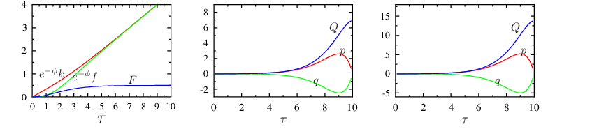
So the numerical solution tells us, if on any point, including the boundary point and , the constraint (54) is not obeyed55 5 Although our boundary condition satisfy the constraint (54), since , and satisfy different equations as , and , they will make the complete , and do not satisfy eqs(54) in the internal point., they will not be obeyed in the internal region of . But if we are interested in the small region, then regardless of the boundary, we can always take the eq(54) as a valid constraint.
From reference [7], we know that, the duality cascading can be ascribed to the varying of effective D3-brane charges with respect to the holographic radial coordinate. By the effective D3-brane charge definition of [21],
| (74) |
we know that, if the functions , and deviate from BCCNR’s results, then the corresponding duality cascading should also be different from that of BCCNR. We displayed in Figure 3 the dependence of the effective D3-brane charges on the radial coordinate. From the figure we see that, although the deviation of functions , and deviate from BCCNR’s result remarkably in the large region, the corresponding does not do so. As the conclusion, we say that discarding the constraint eq(54) does not change the dual cascading described by reference [21] qualitatively.

3.2 Extension of BCCNR-KS solution — beyond the duality wall
This section we study the extension of BCCNR flavored KS solution into negative coupling constant region.
First, we note that in the KS solution, the sensible region of the radial coordinate is 66 6 Only from the metric functions, we cannot look this out. This fact is necessary to assure the positivity of the form fields in the KS theory.. While in BCCNR’s solution, to assure the reality of the dilaton field, the sensible value of coordinate is . If we allow the string coupling can take negative values, or equivalently the dilaton field can carry an imaginary part of , then we can extend BCCNR’s solution into the region:
| (75) |
The sign choice here is similar to that in eq(2.2), i.e., when the “” sign appears, the “” sign is for the part of the relevant expressions while the “” sign is for the part. Also similar to the requirement there, we require and simultaneously so that super-gravity descriptions at the point is valid. Obviously, when one goes across the point, the amplitude of the string coupling is continuous, but its phase jumps by , . We assume that, in the negative coupling constant region , as long as and , then super-gravity descriptions are still valid.

On the dual gauge theory side, the negative string coupling constant means that the gauge coupling constants are also negative. Or equivalently, the gauge coupling constants carry imaginary part of . Just as we expressed in the previous sections, we are not sure the existence of physical mechanism which can transmute this imaginary part into the gauge theory parameter, and make the negative coupling constants sensible concepts. We just simply assume that the negative coupling constants are just as physical as positive ones, and both the super-gravity descriptions and the AdS/CFT correspondence are valid. Under this assumption, BCCNR’s duality cascading can be extended beyond the duality wall marked by the radial coordinate . We displayed in Figure 4 the extended duality cascading picture. From this figure we see that, below the duality wall, the slope of the versus energy scale becomes larger and larger as RG flows up. However, as long as it goes beyond the duality all, the trend reverses.
Second, we consider the extension of BCCNR’s metric functions , , . Construct the following combinations,
| (76) |
where describes the relative size of the two factors in the base space of a deformed conifold which has the topology of a fibre over base ; is related to the total volume of the conifold; while corresponds to the squashing of the fibre of the base relative to the factor. Integration of these equations should distinguish three different cases. The first is when , this case will give metric functions of the KT solution, which is equivalent to those of the previous section. The second case is when , the last one is when . Since the two factor s of the conifold’s base is symmetric, the metric functions in the case of can be obtained from those of the by simply interchanging the position of the two factors. Considering this fact, we will assume that in the following. Under this assumption, the solution to eq(76) can be written as
| (77a) | |||
| (77b) | |||
| (77c) | |||
where , and are integration constants. specifies the relative size between the two factors in the conifold’s base space at point. is related to the total volume of the conifold’s base at . It plays the same role as the parameter does in the eqs(3.7) of reference [21]. specifies the relative size of the bundle to the factor at point. The constant can always be set to zero by translating redefinition of the coordinate. We will do so in the following. In this case, if , , otherwise diverges at the point.

Substituting eqs(77) into (76) and setting , we get manifest expressions for the metric functions
| (78a) | |||
| (78b) | |||
| (78c) | |||
| (78d) | |||
If we set and restrict the sensible region of to be , then the above expressions reduce to the equations (3.6-3.7) of reference [21]. We display in figure 5 numerical behaviors of the three metric functions and their ratios/products. From the figure, we see that on the transition point between the negative and positive coupling constant region , the metric functions are continuous but not smooth. Nevertheless, since the form fields are not continuous at this point, see the following, the super-gravity background as a whole is discontinuous. So if the the negative coupling region is physical and it is connected with the positive coupling region through a phase transition, then the transition is a first order one.

Finally, we turn to the extension of the flavored form fields. If we simply extend BCCNR’s form fields solution into the negative coupling constant region , then their expressions are completely the same as eqs(3.1), but with the radial coordinate taking values in the region. This kind of form fields will make the effective D3-brane charges ,defined by eq(74), in the be negative, please see Figure 6. However, if we allow the flavored form fields (, and ) can be different from the unflavored ones (, and ), see eqs(71), then the difference , and will satisfy eqs(72). Letting them be infinitesimal fractions of , and on the boundary and , they will become very large relative to the latter ones in the middle region. On the point , when this , and corrections are included, the resulting form fields even become discontinuous functions of . A very interesting facts is, when these corrections are included, the resulting effective D3-branes charge become positive in the whole region, please see Figure 6 77 7 On the boundary point and , the effective D3-branes charge is zero..
With the above extended metric functions , and form fields solution , and , we can get the warp factor by simply substituting them into eq(52) and make the integration. To this point, we finish the extension of BCCNR’s flavored KS geometry to the negative coupling constant regions. For comparisons with the extended BCCNR-KW geometry and for future references, we calculated the ricci scalar of the BCCNR flavored KS geometry. The result is as follows,
| (79) |
| (80) |
From these expressions, we see that, since the appearance of the fractional branes, marked by the parameter , the Ricci scalars do not have the exact form of two order polynomials of . If we study the singular/regular behavior of , we will see that it is regular at but not continuous; it is regular both at and .
4 Conclusions
We extend the BCCNR flavored KW/KS geometries into negative coupling constant region. In the extended BCCNR-KW geometry: the positive coupling constant region preserves all the characters of the original theory; while the negative coupling constant region has the asymptotical geometry of multi D3-branes placed at the apex of the a conifold. The positive and negative coupling constant region have continuous, although not smooth, super-gravity metric but discontinuous coupling constant. In the extended BCCNR-KS geometry: the positive coupling constant region also preserves the main characters of the original theory, but we provide a comment which may be looked as a supplement to BCCNR’s solution in the form fields sector; in the negative coupling constant region, the extended solution asymptotically becomes the unflavored KS geometry. On the point across the positive and negative coupling constant region, the metrics are continuous but non-smoothly connected, the form fields are discontinuous. In our studies, we assume that the negative coupling constant region is just as physical as the positive one, and the two regions are connected through a physical phase transition. One can also assume the existence of some physical mechanisms which can transmute the phase of the negative coupling constant into the corresponding axion field and make the coupling constant become a positive one. Looking for this kind of physical mechanisms may be an interesting topic for future works.
References
- [1] J. M. Maldacena, “The large N limit of superconformal field theories and supergravity”, Adv. Theor. Math. Phys. 2 (1998) 231–252, hep-th/9711200.
- [2] S. S. Gubser, I. R. Klebanov, and A. M. Polyakov, “Gauge theory correlators from non-critical string theory”, Phys. Lett. B428 (1998) 105–114, hep-th/9802109; E. Witten, “Anti-de Sitter space and holography”, Adv. Theor. Math. Phys. 2 (1998) 253–291, hep-th/9802150; “Anti-de Sitter space, thermal phase transition, and confinement in gauge theories,” Adv. Theor. Math. Phys. 2 (1998) 505–532, hep-th/9803131.
- [3] L. Girardello, M. Petrini, M. Porrati and A. Zaffaroni, Nucl. Phys. B 569, 451 (2000); hep-th/9909047. L. Girardello, M. Petrini, M. Porrati and A. Zaffaroni, JHEP 9905, 026 (1999); hep-th/9903026. L. Girardello, M. Petrini, M. Porrati and A. Zaffaroni, JHEP 9812, 022 (1998); hep-th/9810126. D. Z. Freedman, S. S. Gubser, K. Pilch and N. P. Warner, Adv. Theor. Math. Phys. 3, 363 (1999); hep-th/9904017. D. Z. Freedman, S. S. Gubser, K. Pilch and N. P. Warner, JHEP 0007, 038 (2000); hep-th/9906194. J. Polchinski and M. J. Strassler, hep-th/0003136. J. Babington, D. E. Crooks and N. J. Evans, Phys. Rev. D 67, 066007 (2003); hep-th/0210068. J. Babington, D. E. Crooks and N. J. Evans, JHEP 0302, 024 (2003); hep-th/0207076.
- [4] I. R. Klebanov, Edward Witten, “Superconformal field theory on three-branes at a Calabi-Yau singularity”, Nucl. Phys. B536 (1998) 199-218,
- [5] hep-th/9807080; I. R. Klebanov, N. A. Nekrasov, “Gravity duals of fractional branes and logarithmic RG flow”, Ncul. Phys. B574 (2000) 263, hep-th/9911096;
- [6] I. R. Klebanov , A. A. Tseytlin, “Gravity duals of supersymmetric SU(N) x SU(N+M) gauge theories”, Nucl. Phys. B578 (2000) 123, hep-th/0002159;
- [7] I. R. Klebanov, M. J. Strassler, “Supergravity and a confining gauge theory: Duality cascades and chi SB resolution of naked singularities”, JHEP 0008 (2000) 052, hep-th/0007191;
- [8] S. S. Gubser, C. P. Herzog and I. R. Klebanov, “Symmetry breaking and axionic strings in the warped deformed conifold”, JHEP 0409 (2004) 036, hep-th/0405282.
- [9] A. Karch, E. Katz, “Adding flavor to AdS / CFT”, JHEP 0206 (2002) 043, hep-th/0205236
- [10] D. Arean, D. E. Crooks, A. V. Ramallo, “Supersymmetric probes on the conifold”, JHEP 0411 (2004) 035, hep-th/0408210.
- [11]
P. Ouyang,
“Holomorphic D7-branes and flavored gauge theories”,
Nucl. Phys. B699 (2004) 207,
hep-th/0311084;
T. S. Levi and P. Ouyang, “Mesons and flavor on the conifold” hep-th/0506021; - [12]
T. Sakai, J Sonnenschein,
“Probing flavored mesons of confining gauge theories by supergravity”,
JHEP 0309 (2003) 047,
hep-th/0305049;
S. Kuperstein, “Meson spectroscopy from holomorphic probes on the warped deformed conifold”, JHEP 0503 (2005) 014, hep-th/0411097 - [13] B. A. Burrington, J. T. Liu, L. A. Pando Zayas and D. Vaman, “Holographic duals of flavored N=1 super Yang-mills: Beyond the probe approximation”, JHEP 0502 (2005) 022 hep-th/0406207.
- [14] B. A. Burrington, V. S. Kaplunovsky and J. Sonnenschein, “Localized Backreacted Flavor Branes in Holographic QCD”, hep-th/0708.1234.
- [15] F. Bigazzi, R. Casero, A. L. Cotrone, E. Kiritsis and A. Paredes, “Non-critical holography and four-dimensional CFT’s with fundamentals”, JHEP 0510 (2005) 012 hep-th/0505140.
- [16] R. Casero, C. Nunez and A. Paredes, “Towards the string dual of N = 1 SQCD-like theories”, Phys. Rev. D73 (2006) 086005 hep-th/0602027.
- [17] A. Paredes, “On unquenched N = 2 holographic flavor”, JHEP 0612 (2006) 032 hep-th/0610270.
- [18] S. Murthy and J. Troost, “D-branes in non-critical superstrings and duality in N = 1 gauge theories with flavor”, JHEP 0610 (2006) 019 hep-th/0606203.
- [19] R. Casero and A. Paredes, “A note on the string dual of N = 1 SQCD-like theories”, hep-th/0701059.
- [20] F. Benini, F Canoura, S. Cremonesi, C. Nunez, A. V. Ramallo, “Unquenched flavors in the Klebanov-Witten model”, JHEP 0702 : (2007)090, hep-th/0612118
- [21] F. Benini, F Canoura, S. Cremonesi, C. Nunez, A. V. Ramallo, “Backreacting flavors in the Klebanov-Strassler background”, 0706.1238
- [22] “Holographic phase transitions with fundamental matter”, D. Mateos, R. C. Myers, R. M. Thomson, Phys.Rev.Lett. 97 (2006) 091601 0605046v2., “Deconfinement phase transition in holographic QCD with matter”, Y. Kim, B.-H Lee, S. Nam, C. Park, S.-J Sin 0706.2525v1.
- [23] R. Apreda, J. Erdmenger, D. Lust, C. Sieg, “Adding flavour to the Polchinski-Strassler background”, 0610276v1.
- [24] C. Sieg, “Holographic flavour in the N=1 Polchinski-Strassler background”, 0706.3544v1
- [25] “Holographic flavor on the Higgs branch”, D. Arean, A. V. Ramallo and D. Rodriguez-Gomez, JHEP 0705 (2007) 044 0703094v2