Convolutional Entanglement Distillation
Abstract
We develop a theory of entanglement distillation that exploits a convolutional coding structure. We provide a method for converting an arbitrary classical binary or quaternary convolutional code into a convolutional entanglement distillation protocol. The imported classical convolutional code does not have to be dual-containing or self-orthogonal. The yield and error-correcting properties of such a protocol depend respectively on the rate and error-correcting properties of the imported classical convolutional code. A convolutional entanglement distillation protocol has several other benefits. Two parties sharing noisy ebits can distill noiseless ebits “online” as they acquire more noisy ebits. Distillation yield is high and decoding complexity is simple for a convolutional entanglement distillation protocol. Our theory of convolutional entanglement distillation reduces the problem of finding a good convolutional entanglement distillation protocol to the well-established problem of finding a good classical convolutional code.
Index Terms:
quantum convolutional codes, convolutional entanglement distillation, quantum information theory, entanglement-assisted quantum codes, catalytic codesI Introduction
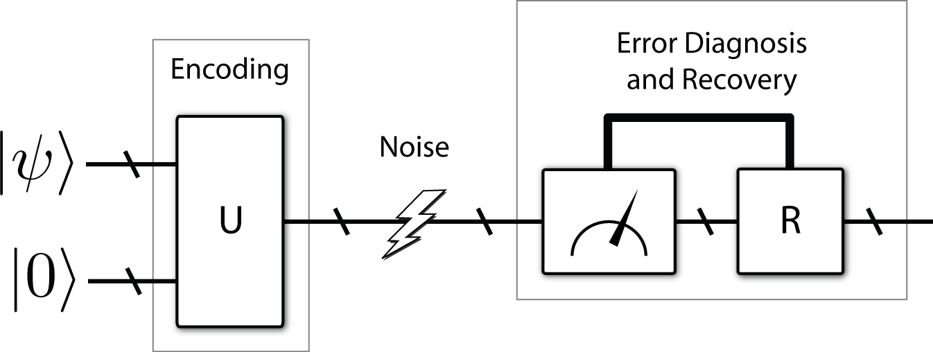
The theory of quantum error correction [1, 2, 3, 4, 5] plays a prominent role in the practical realization and engineering of quantum computing and communication devices. The first quantum error-correcting codes [1, 2, 3, 5] are strikingly similar to classical block codes [6] in their operation and performance. Quantum error-correcting codes restore a noisy, decohered quantum state to a pure quantum state. A stabilizer [4] quantum error-correcting code appends ancilla qubits to qubits that we want to protect. A unitary encoding circuit rotates the global state into a subspace of a larger Hilbert space. This highly entangled, encoded state corrects for local noisy errors. Figure 1 illustrates the above procedures for encoding a stabilizer code. A quantum error-correcting code makes quantum computation and quantum communication practical by providing a way for a sender and receiver to simulate a noiseless qubit channel given a noisy qubit channel that has a particular error model.
The stabilizer theory of quantum error correction allows one to import some classical binary or quaternary codes for use as a quantum code. The only “catch” when importing is that the classical code must satisfy the dual-containing or self-orthogonality constraint. Researchers have found many examples of classical codes satisfying this constraint [5], but most classical codes do not.
Brun, Devetak, and Hsieh extended the standard stabilizer theory of quantum error correction by developing the entanglement-assisted stabilizer formalism [7, 8]. They included entanglement as a resource that a sender and receiver can exploit for a quantum error-correcting code. They provided a “direct-coding” construction in which a sender and receiver can use ancilla qubits and ebits11 1 An ebit is a nonlocal bipartite Bell state . in a quantum code. Gottesman later showed that their construction is optimal [9]—it gives the minimum number of ebits required for the entanglement-assisted quantum code. The benefit of including shared entanglement is that one can import an arbitrary classical binary or quaternary code for use as an entanglement-assisted quantum code. Another benefit of using shared entanglement, in addition to being able to import an arbitrary classical linear code, is that the performance of the original classical code determines the performance of the resulting quantum code. The entanglement-assisted stabilizer formalism thus is a significant and powerful extension of the stabilizer formalism.
The goal of entanglement distillation resembles the goal of quantum error correction [10, 11]. An entanglement distillation protocol extracts noiseless, maximally-entangled ebits from a larger set of noisy ebits. A sender and receiver can use these noiseless ebits as a resource for several quantum communication protocols [12, 13].
Bennett et al. showed that a strong connection exists between quantum error-correcting codes and entanglement distillation and demonstrated a method for converting an arbitrary quantum error-correcting code into a one-way entanglement distillation protocol [11]. A one-way entanglement distillation protocol utilizes one-way classical communication between sender and receiver to carry out the distillation procedure. Shor and Preskill improved upon Bennett et al.’s method by avoiding the use of ancilla qubits and gave a simpler method for converting an arbitrary CSS quantum error-correcting code into an entanglement distillation protocol [14]. Nielsen and Chuang showed how to convert a stabilizer quantum error-correcting code into a stabilizer entanglement distillation protocol [15]. Luo and Devetak then incorporated shared entanglement to demonstrate how to convert an entanglement-assisted stabilizer code into an entanglement-assisted entanglement distillation protocol [16]. All of the above constructions exploit the relationship between quantum error correction and entanglement distillation—we further exploit the connection in this paper by forming a convolutional entanglement distillation protocol.
Several authors have recently contributed toward a theory of quantum convolutional codes [17, 18, 19, 20]. Quantum convolutional codes are useful in a communication context where a sender has a large stream of qubits to send to a receiver. Quantum convolutional codes are similar to classical convolutional codes in their operation and performance [18, 20]. Classical convolutional codes have some advantages over classical block codes such as superior code rates and lower decoding complexity [21]. Their quantum counterparts enjoy these same advantages over quantum block codes [20].
The development of quantum convolutional codes has been brief but successful. Chau was the first to construct some quantum convolutional codes [22, 23], though some authors [20] argue that his construction is not a true quantum convolutional code. Several authors have established a working theory of quantum convolutional coding based on the stabilizer formalism and classical self-orthogonal codes over the finite field [17, 18, 19, 20]. Others have also provided a practical way for realizing “online” encoding and decoding circuits for quantum convolutional codes [17, 18, 24, 25]. These successes have led to a theory of quantum convolutional coding which is useful but not complete. We add to the usefulness of the quantum convolutional theory by considering entanglement distillation and shared entanglement.
In this paper, our main contribution is a theory of convolutional entanglement distillation. Our theory allows us to import the entirety of classical convolutional coding theory for use in entanglement distillation. The task of finding a good convolutional entanglement distillation protocol now becomes the well-established task of finding a good classical convolutional code.
We begin in Section 5 by showing how to construct a convolutional entanglement distillation protocol from an arbitrary quantum convolutional code. We translate earlier protocols [14, 15] for entanglement distillation of a block of noisy ebits to the convolutional setting. Our convolutional entanglement distillation protocol possesses several benefits—it has a higher distillation yield and lower decoding complexity than a block entanglement distillation protocol. A convolutional entanglement distillation protocol has the additional benefit of distilling entanglement “online.” This online property is useful because the sender and receiver can distill entanglement “on the fly” as they obtain more noisy ebits. This translation from a quantum convolutional code to an entanglement distillation protocol is useful because it paves the way for our major contribution.
Our major advance is a method for constructing a convolutional entanglement distillation protocol when the sender and receiver initially share some noiseless ebits. All prior quantum convolutional work requires the code to satisfy the restrictive self-orthogonality constraint, and authors performed specialized searches for classical convolutional codes that meet this constraint [17, 18, 19, 20]. We lift this constraint by allowing shared noiseless entanglement. The benefit of convolutional entanglement distillation with entanglement assistance is that we can import an arbitrary classical binary or quaternary convolutional code for use in a convolutional entanglement distillation protocol. The error-correcting properties for the convolutional entanglement distillation protocol follow directly from the properties of the imported classical code. Thus we can apply the decades of research on classical convolutional coding theory with many of the benefits of the convolutional structure carrying over to the quantum domain.
We organize our work as follows. In Section II, we review the stabilizer theory for quantum error correction and entanglement distillation. The presentation of the mathematics is similar in style to Refs. [20, 8]. The stabilizer review includes a review of the standard stabilizer theory (Section II-A), the entanglement-assisted stabilizer theory (Section II-B), convolutional stabilizer codes (Section II-C), stabilizer entanglement distillation (Section II-D), and entanglement-assisted entanglement distillation (Section II-E). We provide a small contribution in the Appendix—a simple algorithm to determine an encoding circuit and the optimal number of ebits required for an entanglement-assisted block code. The original work [8] gave two theorems relevant to the encoding circuit, but the algorithm we present here is simpler. In Section 5, we show how to convert an arbitrary quantum convolutional code into a convolutional entanglement distillation protocol. In Section IV, we provide several methods and examples for constructing convolutional entanglement distillation protocols where two parties possess a few initial noiseless ebits. These initial noiseless ebits act as a catalyst for the convolutional distillation protocol. The constructions in Section IV make it possible to import an arbitrary classical binary or quaternary convolutional code for use in convolutional entanglement distillation.
II Review of the Stabilizer Formalism
II-A Standard Stabilizer Formalism for Quantum Block Codes
The stabilizer formalism exploits elements of the Pauli group in formulating quantum error-correcting codes. The set consists of the Pauli operators:
The above operators act on a single qubit—a state in a two-dimensional Hilbert space. Operators in have eigenvalues and either commute or anti-commute. The set consists of -fold tensor products of Pauli operators:
| (1) |
Elements of act on a quantum register of qubits. We occasionally omit tensor product symbols in what follows so that . The -fold Pauli group plays an important role for both the encoding circuit and the error-correction procedure of a quantum stabilizer code over qubits.
Let us define an stabilizer quantum error-correcting code to encode logical qubits into physical qubits. The rate of such a code is . Its stabilizer is an abelian subgroup of the -fold Pauli group : . does not contain the operator . The simultaneous -eigenspace of the operators constitutes the codespace. The codespace has dimension so that we can encode qubits into it. The stabilizer has a minimal representation in terms of independent generators . The generators are independent in the sense that none of them is a product of any other two (up to a global phase). The operators function in the same way as a parity check matrix does for a classical linear block code. Figure 1 illustrates the operation of a stabilizer code.
One of the fundamental notions in quantum error correction theory is that it suffices to correct a discrete error set with support in the Pauli group [1]. Suppose that the errors affecting an encoded quantum state are a subset of the Pauli group : . An error that affects an encoded quantum state either commutes or anticommutes with any particular element in . The error is correctable if it anticommutes with an element in . An anticommuting error is detectable by measuring each element in and computing a syndrome identifying . The syndrome is a binary vector with length whose elements identify whether the error commutes or anticommutes with each . An error that commutes with every element in is correctable if and only if it is in . It corrupts the encoded state if it commutes with every element of but does not lie in . So we compactly summarize the stabilizer error-correcting conditions: a stabilizer code can correct any errors in if or where is the centralizer of .
II-B Entanglement-Assisted Stabilizer Formalism
The entanglement-assisted stabilizer formalism extends the standard stabilizer formalism by including shared entanglement [7, 8]. Figure 2 demonstrates the operation of a generic entanglement-assisted stabilizer code.
The advantage of entanglement-assisted stabilizer codes is that the sender can exploit the error-correcting properties of an arbitrary set of Pauli operators. The sender’s Pauli operators do not necessarily have to form an abelian subgroup of . The sender can make clever use of her shared ebits so that the global stabilizer is abelian and thus forms a valid quantum error-correcting code.

We review the construction of an entanglement-assisted code. Suppose that there is a nonabelian subgroup of size . Application of the fundamental theorem of symplectic geometry22 2 We loosely refer to this theorem as the fundamental theorem of symplectic geometry because of its importance in symplectic geometry and in quantum coding theory. [26] (Lemma 1 in [7]) states that there exists a minimal set of independent generators for with the following commutation relations:
| (2) |
The decomposition of into the above minimal generating set determines that the code requires ancilla qubits and ebits. The code requires an ebit for every anticommuting pair in the minimal generating set. The simple reason for this requirement is that an ebit is a simultaneous -eigenstate of the operators . The second qubit in the ebit transforms the anticommuting pair into a commuting pair . The above decomposition also minimizes the number of ebits required for the code [9]—it is an optimal decomposition.
We can partition the nonabelian group into two subgroups: the isotropic subgroup and the entanglement subgroup . The isotropic subgroup is a commuting subgroup of and thus corresponds to ancilla qubits: . The elements of the entanglement subgroup come in anticommuting pairs and thus correspond to ebits: .
The two subgroups and play a role in the error-correcting conditions for the entanglement-assisted stabilizer formalism. An entanglement-assisted code corrects errors in a set if for all , .
The operation of an entanglement-assisted code is as follows. The sender performs an encoding unitary on her unprotected qubits, ancilla qubits, and her half of the ebits. The unencoded state is a simultaneous +1-eigenstate of the following operators:
| (3) |
The operators to the right of the vertical bars indicate the receiver’s half of the shared ebits. The encoding unitary transforms the unencoded operators to the following encoded operators:
| (4) |
The sender transmits all of her qubits over the noisy quantum channel. The receiver then possesses the transmitted qubits and his half of the ebits. He measures the above encoded operators to diagnose the error. The last step is to correct for the error.
We give an example of an entanglement-assisted stabilizer code in the Appendix. This example highlights the main features of the theory given above.
The Appendix also gives an original algorithm that determines the encoding circuit for the sender to perform. The algorithm determines the number of ancilla qubits and the number of ebits that the code requires.
The defined rate of an entanglement-assisted quantum error-correcting code is [7, 8]. The authors defined the rate in this way to compare entanglement-assisted codes with standard quantum error-correcting codes.
We mention that the rate pair more properly characterizes the rate of an entanglement-assisted code because an entanglement-assisted code is a “father” code in the sense of Ref. [27]. The first number in the pair gives the rate of noiseless qubits generated per channel use and the second number gives the rate of ebits consumed per channel use. The rate pair falls in the two-dimensional capacity region for the “father” protocol. The goal of an entanglement-assisted coding strategy is for the rate pair to approach the boundary of the capacity region as the block length becomes large.
II-C Convolutional Stabilizer Codes
The block codes reviewed above are useful in quantum computing and in quantum communications. The encoding circuit for a large block code typically has a high complexity although those for modern codes do have lower complexity.
Quantum convolutional coding theory [17, 18, 19, 20] offers a different paradigm for coding quantum information. The convolutional structure is useful for a quantum communication scenario where a sender possesses a stream of qubits to send to a receiver. The encoding circuit for a quantum convolutional code has a much lower complexity than an encoding circuit needed for a large block code. It also has a repetitive pattern so that the same physical devices or the same routines can manipulate the stream of quantum information.
Quantum convolutional stabilizer codes borrow heavily from the structure of their classical counterparts [17, 18, 19, 20]. Quantum convolutional codes are similar because some of the qubits feed back into a repeated encoding unitary and give the code a memory structure like that of a classical convolutional code. The quantum codes feature online encoding and decoding of qubits. This feature gives quantum convolutional codes both their low encoding and decoding complexity and their ability to correct a larger set of errors than a block code with similar parameters.
We first review some preliminary mathematics and follow with the definition of a quantum convolutional stabilizer code [18, 20]. We end this section with a brief discussion of encoding circuits for quantum convolutional codes.
A quantum convolutional stabilizer code acts on a Hilbert space that is a countably infinite tensor product of two-dimensional qubit Hilbert spaces where
| (5) |
and . A sequence of Pauli matrices , where
| (6) |
can act on states in . Let denote the set of all Pauli sequences. The support supp of a Pauli sequence is the set of indices of the entries in that are not equal to the identity. The weight of a sequence is the size of its support. The delay del of a sequence is the smallest index for an entry not equal to the identity. The degree deg of a sequence is the largest index for an entry not equal to the identity. E.g., the following Pauli sequence
| (7) |
has support , weight three, delay one, and degree four. A sequence has finite support if its weight is finite. Let denote the set of Pauli sequences with finite support. The following definition for a quantum convolutional code utilizes the set in its description.
Definition 1
A rate -convolutional stabilizer code with is a commuting set of all -qubit shifts of a basic generator set . The basic generator set has Pauli sequences of finite support:
| (8) |
The constraint length of the code is the maximum degree of the generators in . A frame of the code consists of qubits.
Remark 1
The above definition requires that all elements of commute. In Section IV, we lift the restrictive commutative condition when we construct a convolutional entanglement distillation protocol with entanglement assistance.
A quantum convolutional code admits an equivalent definition in terms of the delay transform or -transform. The -transform captures shifts of the basic generator set . Let us define the -qubit delay operator acting on any Pauli sequence as follows:
| (9) |
We can write repeated applications of as a power of :
| (10) |
Let be the set of shifts of elements of by . Then the full stabilizer for the convolutional stabilizer code is
| (11) |

Figure 3 outlines the operation of a convolutional stabilizer code. The protocol begins with the sender encoding a stream of qubits with an online encoding circuit such as that given in [25]. The encoding circuit is “online” if it acts on a few blocks of qubits at a time. The sender transmits a set of qubits as soon as the first unitary finishes processing them. The receiver measures all the generators in and corrects for errors as he receives the online encoded qubits. He finally decodes the encoded qubits with a decoding circuit. The qubits decoded from this convolutional procedure should be error free and ready for quantum computation at the receiving end.
A finite-depth circuit maps a Pauli sequence with finite weight to one with finite weight [18]. It does not map a Pauli sequence with finite weight to one with infinite weight. This property is important because we do not want the decoding circuit to propagate uncorrected errors into the information qubit stream [21]. A finite-depth decoding circuit corresponding to the stabilizer exists by the algorithm given in [25].
Example 1
Forney et al. provided an example of a rate-1/3 quantum convolutional code by importing a particular classical quaternary convolutional code [19, 20]. Grassl and Rötteler determined a noncatastrophic encoding circuit for Forney et al.’s rate-1/3 quantum convolutional code [25]. The basic stabilizer and its first shift are as follows:
| (12) |
The code consists of all three-qubit shifts of the above generators. The vertical bars are a visual aid to illustrate the three-qubit shifts of the basic generators. The code can correct for an arbitrary single-qubit error in every other frame.
II-D Stabilizer Entanglement Distillation without Entanglement Assistance
The purpose of an entanglement distillation protocol is to distill pure ebits from noisy ebits where [10, 11]. The yield of such a protocol is . Two parties can then use the noiseless ebits for quantum communication protocols. Figure 4 illustrates the operation of a block entanglement distillation protocol.

The two parties establish a set of shared noisy ebits in the following way. The sender Alice first prepares Bell states locally. She sends the second qubit of each pair over a noisy quantum channel to a receiver Bob. Let be the state rearranged so that all of Alice’s qubits are on the left and all of Bob’s qubits are on the right. The noisy channel applies a Pauli error in the error set to the set of qubits sent over the channel. The sender and receiver then share a set of noisy ebits of the form where the identity acts on Alice’s qubits and is some Pauli operator in acting on Bob’s qubits.
A one-way stabilizer entanglement distillation protocol uses a stabilizer code for the distillation procedure. Figure 4 highlights the main features of a stabilizer entanglement distillation protocol. Suppose the stabilizer for an quantum error-correcting code has generators . The distillation procedure begins with Alice measuring the generators in . Let be the set of the projectors that project onto the orthogonal subspaces corresponding to the generators in . The measurement projects randomly onto one of the subspaces. Each commutes with the noisy operator on Bob’s side so that
| (13) |
The following important “Bell-state matrix identity” holds for an arbitrary matrix :
| (14) |
Then (13) is equal to the following:
| (15) |
Therefore each of Alice’s projectors projects Bob’s qubits onto a subspace corresponding to Alice’s projected subspace . Alice restores her qubits to the simultaneous +1-eigenspace of the generators in . She sends her measurement results to Bob. Bob measures the generators in . Bob combines his measurements with Alice’s to determine a syndrome for the error. He performs a recovery operation on his qubits to reverse the error. He restores his qubits to the simultaneous +1-eigenspace of the generators in . Alice and Bob both perform the decoding unitary corresponding to stabilizer to convert their logical ebits to physical ebits.
II-E Stabilizer Entanglement Distillation with Entanglement Assistance
Luo and Devetak provided a straightforward extension of the above protocol [16]. Their method converts an entanglement-assisted stabilizer code into an entanglement-assisted entanglement distillation protocol.
Luo and Devetak form an entanglement distillation protocol that has entanglement assistance from a few noiseless ebits. The crucial assumption for an entanglement-assisted entanglement distillation protocol is that Alice and Bob possess noiseless ebits in addition to their noisy ebits. The total state of the noisy and noiseless ebits is
| (16) |
where is the identity matrix acting on Alice’s qubits and the noisy Pauli operator affects Bob’s first qubits only. Thus the last ebits are noiseless, and Alice and Bob have to correct for errors on the first ebits only.
The protocol proceeds exactly as outlined in the previous section. The only difference is that Alice and Bob measure the generators in an entanglement-assisted stabilizer code. Each generator spans over qubits where the last qubits are noiseless.
We comment on the yield of this entanglement-assisted entanglement distillation protocol. An entanglement-assisted code has generators that each have Pauli entries. These parameters imply that the entanglement distillation protocol produces ebits. But the protocol consumes initial noiseless ebits as a catalyst for distillation. Therefore the yield of this protocol is .
In Section IV, we exploit this same idea of using a few noiseless ebits as a catalyst for distillation. The idea is similar in spirit to that developed in this section, but the mathematics and construction are different because we perform distillation in a convolutional manner.
III Convolutional Entanglement Distillation without Entanglement Assistance

We now show how to convert an arbitrary quantum convolutional code into a convolutional entanglement distillation protocol. Figure 5 illustrates an example of a yield-1/3 convolutional entanglement distillation protocol. The protocol has the same benefits as a quantum convolutional code: an online decoder with less decoding complexity than a block protocol, good error-correcting properties, and higher ebit yield than a block protocol. The protocol we develop in this section is useful for our major contribution presented in the next section.
We can think of our protocol in two ways. Our protocol applies when a sender Alice and a receiver Bob possess a countably infinite number of noisy ebits. Our protocol also applies as an online protocol when Alice and Bob begin with a finite number of noisy ebits and establish more as time passes. The countably infinite and online protocols are equivalent. We would actually implement the entanglement distillation protocol in the online manner, but we formulate the forthcoming mathematics with the countably infinite description. Each step in the protocol does not need to wait for the completion of its preceding step if Alice and Bob employ the protocol online.
The protocol begins with Alice and Bob establishing a set of noisy ebits. Alice prepares a countably infinite number of Bell states locally. She sends one half of each Bell state through a noisy quantum channel. Alice and Bob then possess a state that is a countably infinite number of noisy ebits where
| (17) |
The state is equivalent to the following ensemble
| (18) |
In the above, is the probability that the state is ,
| (19) |
and is the state rearranged so that all of Alice’s qubits are on the left and all of Bob’s are on the right. is a Pauli sequence of errors acting on Bob’s side. These errors result from the noisy quantum channel. is a sequence of identity matrices acting on Alice’s side indicating that the noisy channel does not affect her qubits. Alice and Bob need to correct for a particular error set in order to distill noiseless ebits.
Alice and Bob employ the following strategy to distill noiseless ebits. Alice measures the generators in the basic set . The measurement operation projects the first ebits ( is the constraint length) randomly onto one of orthogonal subspaces. Alice places the measurement outcomes in an -dimensional classical bit vector . She restores her half of the noisy ebits to the simultaneous +1-eigenspace of the generators in if differs from the all-zero vector. She sends to Bob over a classical communications channel. Bob measures the generators in and stores the measurement outcomes in a classical bit vector . Bob compares to by calculating an error vector . He corrects for any errors that can identify. He may have to wait to receive later error vectors before determining the full error syndrome. He restores his half of the noisy ebits to the simultaneous +1-eigenspace of the generators in if the bit vector indicates that his logical ebits are not in the +1-space. Alice and Bob repeat the above procedure for all shifts , , … of the basic generators in . Bob obtains a set of classical error vectors : . Bob uses a maximum-likelihood decoding technique such as Viterbi decoding [28] or a table-lookup on the error set to determine which errors occur. This error determination process is a purely classical computation. He reverses all errors after determining the syndrome.
The states that Alice and Bob possess after the above procedure are encoded logical ebits. They can extract physical ebits from these logical ebits by each performing the online decoding circuit for the code . The algorithm outlined in [25] gives a method for determining the online decoding circuit.
Example 2
We use the rate-1/3 quantum convolutional code in Example 1 to produce a yield-1/3 convolutional entanglement distillation protocol. Alice measures the generators in the stabilizer in (12) for every noisy ebit she shares with Bob. Alice communicates the result of her measurement of the first two generators to Bob. Alice restores the qubits on her side to be in the simultaneous +1-eigenspace of the first two generators. Bob measures the same first two generators. Alice measures the next two generators, communicates her results, etc. Bob compares his results to Alice’s to determine the error bit vectors. Bob performs Viterbi decoding on the measurement results and corrects for errors. He rotates his states to the simultaneous +1-eigenspace of the generators. Alice and Bob perform the above procedure in an online manner according to Figure 5. Alice and Bob can decode the first six qubits after measuring the second two generators. They can decode because there is no overlap between the first two generators and any two generators after the second two generators. They use the circuit from [25] in reverse order to decode physical ebits from logical ebits. They distill ebits with yield 1/3 by using this convolutional entanglement distillation protocol. The ebit yield of 1/3 follows directly from the code rate of 1/3.
IV Convolutional Entanglement Distillation with Entanglement Assistance
The convolutional entanglement distillation protocol that we develop in this section operates identically to the one developed in the previous section. The measurements, classical communication, and recovery and decoding operations proceed exactly as Figure 5 indicates.
The difference between the protocol in this section and the previous one is that we now assume the sender and receiver share a few initial noiseless ebits. They use these initial ebits as a catalyst to get the protocol started. The sender and receiver require noiseless ebits for each round of the convolutional entanglement distillation protocol. They can use the noiseless ebits generated by earlier rounds for consumption in later rounds. It is possible to distill noiseless ebits in this way by catalyzing the process with a few noiseless ebits. The protocol we develop in this section is a more powerful generalization of the previous section’s protocol.
The construction in this section allows sender and receiver to use an arbitrary set of Paulis for the distillation protocol. The set does not necessarily have to be a commuting set of Paulis. The idea is similar in spirit to entanglement-assisted quantum error correction [7, 8].
The implication of the construction in this section is that we can import an arbitrary binary or quaternary classical convolutional code for use as a quantum convolutional code. We explicitly give some examples to highlight the technique for importing. The error-correcting properties and yield translate directly from the properties of the classical convolutional code. Thus the problem of finding a good convolutional entanglement distillation protocol reduces to that of finding a good classical convolutional code.
We first review some mathematics concerning the commutative properties of quantum convolutional codes. We then present our different constructions for a convolutional entanglement distillation protocol that use entanglement assistance.
IV-A Commutative Properties of Quantum Convolutional Codes
We consider the commutative properties of quantum convolutional codes. We develop some mathematics that leads to the important “shifted symplectic product.” The shifted symplectic product reveals the commutation relations of an arbitrary number of shifts of a set of Pauli sequences. All of our constructions following this preliminary section exploit the properties of the shifted symplectic product.
We first define the phase-free Pauli group on a sequence of qubits. Recall that the delay transform in (9) shifts a Pauli sequence to the right by . Let us assume for now that . Let denote the set of all countably infinite Pauli sequences. The set is equivalent to the set of all one-qubit shifts of arbitrary Pauli operators:
| (20) |
We remark that . We make this same abuse of notation in what follows. We can define the equivalence class of phase-free Pauli sequences:
| (21) |
We develop a relation between binary polynomials and Pauli sequences that is useful for representing the shifting nature of quantum convolutional codes. Suppose and are arbitrary finite-degree and finite-delay polynomials in over
| (22) | ||||
| (23) |
where del, del, deg, deg. Suppose
| (24) |
where indicates the direct product . Let us employ the following shorthand:
| (25) |
Let be a map from the binary polynomials to the Pauli sequences, , where
| (26) |
Let where . The map induces an isomorphism
| (27) |
because addition of binary polynomials is equivalent to multiplication of Pauli elements up to a global phase:
| (28) |
The above isomorphism is a powerful way to capture the infiniteness and shifting nature of convolutional codes with finite-degree and finite-delay polynomials over the binary field .
Recall from Definition 1 that a commuting set comprising a basic set of Paulis and all their shifts specifies a quantum convolutional code. How can we capture the commutation relations of a Pauli sequence and all of its shifts? The shifted symplectic product , where
| (29) |
is an elegant way to do so. The shifted symplectic product maps two vectors and to a binary polynomial with finite delay and finite degree:
| (30) |
The symplectic orthogonality condition originally given in Ref. [18] inspires the definition for the shifted symplectic product. The shifted symplectic product is not a proper symplectic product because it fails to be alternating [26]. The alternating property requires that
| (31) |
but we find instead that the following holds:
| (32) |
Every vector is self-time-reversal antisymmetric with respect to :
| (33) |
Every binary vector is also self-time-reversal symmetric with respect to because addition and subtraction are the same over . We employ the addition convention from now on and drop the minus signs. The shifted symplectic product is a binary polynomial in . We write its coefficients as follows:
| (34) |
The coefficient captures the commutation relations of two Pauli sequences for -qubit shifts of one of the sequences:
| (35) |
Thus two Pauli sequences and commute for all shifts if and only if the shifted symplectic product vanishes.
The next example highlights the main features of the shifted symplectic product and further emphasizes the relationship between Pauli commutation and orthogonality of the shifted symplectic product.
Example 3
Consider two sets of binary polynomials:
We form vectors and from the above polynomials where
| (36) |
The isomorphism maps the above polynomials to the following Pauli sequences:
| (37) |
The vertical bars between every Pauli in the sequence indicate that we are considering one-qubit shifts. We determine the commutation relations of the above sequences by inspection. anticommutes with a shift of itself by one or two to the left or right and commutes with all other shifts of itself. anticommutes with a shift of itself by two or three to the left or right and commutes with all other shifts of itself. anticommutes with shifted to the left by one or two, with the zero-shifted , and with shifted to the right by two or three. The following shifted symplectic products give us the same information:
| (38) |
The nonzero coefficients indicate the commutation relations just as (35) claims.
A quantum convolutional code in general consists of generators with qubits per frame. Therefore, we consider the -qubit extension of the definitions and isomorphism given above. Let the delay transform now shift a Pauli sequence to the right by an arbitrary integer . Consider a -dimensional vector of binary polynomials where . Let us write as follows
where . Suppose
| (39) |
Define a map :
| (40) |
is equivalent to the following map (up to a global phase)
| (41) |
where
| (42) |
Suppose
| (43) |
where . The map induces an isomorphism for the same reasons given in (28):
| (44) |
The isomorphism is again useful because it allows us to perform binary calculations instead of Pauli calculations.
We can again define a shifted symplectic product for the case of -qubits per frame. Let denote the shifted symplectic product between vectors of binary polynomials:
| (45) |
It maps vectors of binary polynomials to a finite-degree and finite-delay binary polynomial
| (46) |
where
The standard inner product gives an alternative way to define the shifted symplectic product:
| (47) |
Every vector is self-time-reversal symmetric with respect to :
| (48) |
The shifted symplectic product for vectors of binary polynomials is a binary polynomial in . We write its coefficients as follows:
| (49) |
The coefficient captures the commutation relations of two Pauli sequences for -qubit shifts of one of the sequences:
| (50) |
Example 4
We consider the case where . Consider the following vectors of polynomials:
| (51) |
Suppose
| (52) |
The isomorphism maps and to the following Pauli sequences:
| (53) |
We can determine the commutation relations by inspection of the above Pauli sequences. anticommutes with itself shifted by one to the left or right, anticommutes with itself shifted by one to the left or right, and anticommutes with shifted by one to the left. The following shifted symplectic products confirm the above commutation relations:
| (54) |
We note two useful properties of the shifted symplectic product . Suppose with . Let us denote scalar polynomial multiplication as follows:
| (55) |
The following identities hold.
| (56) | ||||
| (57) |
We also remark that
iff
We exploit both of the above properties in the constructions that follow.
IV-B Yield (n-1)/n Convolutional Entanglement Distillation with Entanglement Assistance
We present our first method for constructing a convolutional entanglement distillation protocol that uses entanglement assistance. The shifted symplectic product is a crucial component of our formulation.
Suppose Alice and Bob use one generator for an entanglement distillation protocol where
We do not impose a commuting constraint on generator . Alice and Bob choose generator solely for its error-correcting capability.
The shifted symplectic product helps to produce a commuting generator from a noncommuting one. The shifted symplectic product of is
| (58) |
The coefficient for zero shifts is equal to zero because every tensor product of Pauli operators commutes with itself:
| (59) |
Recall that is self-time-reversal symmetric (48). We adopt the following notation for a polynomial that includes the positive-index or negative-index coefficients of the shifted symplectic product :
| (60) | ||||
| (61) |
The following identity holds:
| (62) |
Consider the following vector of polynomials:
| (63) |
Its relations under the shifted symplectic product are the same as :
| (64) |
The vector provides a straightforward way to make commute with all of its shifts. We augment with . The augmented generator is as follows:
| (65) |
The augmented generator has vanishing symplectic product because the shifted symplectic product of nulls the shifted symplectic product of :
| (66) |
The augmented generator commutes with itself for every shift and is therefore useful for convolutional entanglement distillation as outlined in Section 5.
We can construct an entanglement distillation protocol using an augmented generator of this form. The first Pauli entries for every frame of generator correct errors. Entry for every frame of makes commute with every one of its shifts. The error-correcting properties of the code do not include errors on the last (extra) ebit of each frame; therefore, this ebit must be noiseless. It is necessary to catalyze the distillation procedure with noiseless ebits where is the frame size and is the constraint length. The distillation protocol requires this particular amount because it does not correct errors and generate noiseless ebits until it has finished processing the first basic set of generators and of its shifts. Later frames can use the noiseless ebits generated from previous frames. Therefore these initial noiseless ebits are negligible when calculating the yield. This construction allows us to exploit the error-correcting properties of an arbitrary set of Pauli matrices for a convolutional entanglement distillation protocol.
We discuss the yield of such a protocol in more detail. Our construction employs one generator with qubits per frame. The protocol generates noiseless ebits for every frame. But it also consumes a noiseless ebit for every frame. Every frame thus produces a net of noiseless ebits, and the yield of the protocol is .
This yield of is superior to the yield of an entanglement distillation protocol taken from the quantum convolutional codes of Forney et al. [20]. Our construction should also give entanglement distillation protocols with superior error-correcting properties because we have no self-orthogonality constraint on the Paulis in the stabilizer.
It is possible to construct an online decoding circuit for the generator by the methods given in [25]. A circuit satisfies the noncatastrophic property if the polynomial entries of all of the code generators have a greatest common divisor that is a power of the delay operator [25]. The online decoding circuit for this construction obeys the noncatastrophicity property because the augmented generator contains 1 as one of its entries.

Example 5
Suppose we have the following generator
where
The above generator corrects for an arbitrary single-qubit error in a span of eight qubits—four frames. Table I lists the unique syndromes for errors in a single frame. The generator anticommutes with a shift of itself by one or two to the left or right. The shifted symplectic product confirms these commutation relations:
Let us follow the prescription in (65) for augmenting generator . The following polynomial
has the same commutation relations as :
| (71) |
We augment as follows:
The overall generator now looks as follows in the Pauli representation:
The yield of a protocol using the above construction is 1/2. Figure 6 illustrates Bob’s side of the protocol. It shows which of Bob’s half of the ebits are noisy and noiseless, and it gives the measurements that Bob performs.
IV-C Yield (n-m)/n Convolutional Entanglement Distillation with Entanglement Assistance
The construction in the above section uses only one generator for distillation. We generalize the above construction to a code with an arbitrary number of generators. We give an example that illustrates how to convert an arbitrary classical quaternary convolutional code into a convolutional entanglement distillation protocol.
Suppose we have the following generators
where
| (72) |
We make no assumption about the commutation relations of the above generators. We choose them solely for their error-correcting properties.
We again utilize the shifted symplectic product to design a convolutional entanglement distillation protocol with multiple generators. Let us adopt the following shorthand for the auto and cross shifted symplectic product of generators :
| (73) | ||||
| (74) |
Consider the following matrix:
| (75) |
The symplectic relations of the entries are the same as the original :
We mention that the following matrix also has the same symplectic relations:
| (76) |
Let us rewrite (75) as follows:
| (77) |
The above matrix provides a straightforward way to make the original generators commute with all of their shifts. We augment the generators in (72) by the generators to get the following matrix:
Every row of the augmented matrix has vanishing symplectic product with itself and any other row. This condition is equivalent to the following matrix condition for shifted symplectic orthogonality [18]:
| (88) |
The construction gives a commuting set of generators for arbitrary shifts and thus forms a valid stabilizer.
We can readily develop a convolutional entanglement distillation protocol using the above formulation. The generators in the augmented matrix correct for errors on the first ebits. The last ebits are noiseless ebits that help to obtain a commuting stabilizer. It is necessary to catalyze the distillation protocol with noiseless ebits. Later frames can use the noiseless ebits generated from previous frames. These initial noiseless ebits are negligible when calculating the yield.
We comment more on the yield of the protocol. The protocol requires a set of generators with Pauli entries. It generates ebits for every frame. But it consumes noiseless ebits per frame. The net yield of a protocol using the above construction is thus .
The key benefit of the above construction is that we can use an arbitrary set of Paulis for distilling noiseless ebits. This arbitrariness in the Paulis implies that we can import an arbitrary classical convolutional binary or quaternary code for use in a convolutional entanglement distillation protocol.
It is again straightforward to develop a noncatastrophic decoding circuit using previous techniques [25]. Every augmented generator in has 1 as an entry so that it satisfies the property required for noncatastrophicity.
Example 6
We begin with a classical quaternary convolutional code with entries from :
| (89) |
The above code is a convolutional version of the classical quaternary block code from Ref. [7]. We multiply the above generator by and as prescribed in Refs. [5, 20] and use the following map,
| (90) |
to obtain the following Pauli generators
| (91) |
We determine binary polynomials corresponding to the above Pauli generators:
| (92) |
The first generator anticommutes with itself shifted by one to the left or right, the second generator anticommutes with itself shifted by one to the left or right, and the first generator anticommutes with the second shifted by one to the left. The following shifted symplectic products confirm the above commutation relations:
| (93) |
Consider the following two generators:
| (94) |
Their relations under the shifted symplectic product are the same as those in (93).
| (95) |
We use the construction from (76) so that we have positive delay operators in the augmented matrix. We augment the generators and to generators and respectively as follows. The augmented “Z matrix” is
| (96) |
and the augmented “X matrix” is
| (97) |
The augmented matrix is
| (98) |
The first row of is generator and the second row is . The augmented generators have the following Pauli representation.
| (99) |
| (100) |
The original block code from Ref. [7] corrects for an arbitrary single-qubit error. The above entanglement distillation protocol corrects for a single-qubit error in eight qubits—two frames. This error-correcting capability follows from the capability of the block code. The yield of a protocol using the above stabilizer is again 1/2.
IV-D CSS-Like Construction for a Convolutional Entanglement Distillation Protocol
We finally present a construction that allows us to import two arbitrary binary classical codes for use in a convolutional entanglement distillation protocol. The construction is similar to a CSS code because one code corrects for bit flips and the other corrects for phase flips.
We could simply use the technique from the previous section to construct a convolutional entanglement-distillation protocol. We could represent both classical codes as codes over . We could multiply the bit-flip code by and the phase-flip code by and use the above map from to the Paulis. We could then use the above method for augmentation and obtain a valid quantum code for entanglement distillation. But there is a better method that exploits the structure of a CSS code to minimize the number of initial catalytic noiseless ebits.
Our algorithm below uses a Gram-Schmidt like orthogonalization procedure to minimize the number of initial noiseless ebits. The procedure is similar to the algorithm in [8] with some key differences.
Suppose we have generators where
| (101) |
and each vector has length . The above matrix could come from two binary classical codes. The vectors ,…, could come from one code, and the vectors ,…, could come from another code. The following orthogonality relations hold for the above vectors:
| (102) | ||||
| (103) |
We exploit the above orthogonality relations in the algorithm below.
We can perform a Gram-Schmidt process on the above set of vectors. This process orthogonalizes the vectors with respect to the shifted symplectic product. The procedure does not change the error-correcting properties of the original codes because all operations are linear.
The algorithm breaks the set of vectors above into pairs. Each pair consists of two vectors which are symplectically nonorthogonal to each other, but which are symplectically orthogonal to all other pairs. Any remaining vectors that are symplectically orthogonal to all other vectors are collected into a separate set, which we call the set of isotropic vectors. This idea is similar to the decomposition of a vector space into an isotropic and symplectic part. We cannot label the decomposition as such because the shifted symplectic product is not a true symplectic product.
We detail the initialization of the algorithm. Set parameters , , . The index labels the total number of vectors processed, gives the number of pairs, and labels the number of vectors with no partner. Initialize sets and to be null: . keeps track of the pairs and keeps track of the vectors with no partner.
The algorithm proceeds as follows. While , let be the smallest index for a for which . Increment and by one, add to , and proceed to the next round if no such pair exists. Otherwise, swap with . For , perform
| (104) |
if has a purely component. Perform
| (105) |
if has a purely component. Divide every element in by the greatest common factor if the GCF is not equal to one. Then
| (106) |
Increment by one, increment by one, add to , and increment by one. Proceed to the next round.
We now give the method for augmenting the above generators so that they form a commuting stabilizer. At the end of the algorithm, the sets and have the following sizes: and . Let us relabel the vectors for all . We relabel all pairs: call the first and call its partner for all . Call any vector without a partner for all . The relabeled vectors have the following shifted symplectic product relations after the Gram-Schmidt procedure:
| (107) |
where is an arbitrary polynomial. Let us arrange the above generators in a matrix as follows:
| (108) |
We augment the above generators with the following matrix so that all vectors are orthogonal to each other:
| (109) |
The yield of a protocol using the above construction is . Suppose we use an classical binary convolutional code for the bit flips and an classical binary convolutional code for the phase flips. Then the convolutional entanglement distillation protocol has yield .
Example 7
Consider a binary classical convolutional code with the following parity check matrix:
| (110) |
We can use the above parity check matrix to correct both bit and phase flip errors in an entanglement distillation protocol. Our initial quantum parity check matrix is
| (111) |
The shifted symplectic product for the first and second row is . We therefore augment the above matrix as follows:
| (112) |
The above matrix gives a valid stabilizer for use in an entanglement distillation protocol. The yield of a protocol using the above stabilizer is 1/3.
V Conclusion and Current Work
We constructed a theory of convolutional entanglement distillation. The entanglement-assisted protocol assumes that the sender and receiver have some noiseless ebits to use as a catalyst for distilling more ebits. These protocols have the benefit of lifting the self-orthogonality constraint. Thus we are able to import an arbitrary classical convolutional code for use in a convolutional entanglement distillation protocol. The error-correcting properties and rate of the classical code translate to the quantum case. Brun, Devetak, and Hsieh first constructed the method for importing an arbitrary classical block code in their work on entanglement-assisted codes [8, 7]. Our theory of convolutional entanglement distillation paves the way for exploring protocols that approach the optimal distillable entanglement by using the well-established theory of classical convolutional coding.
Convolutional entanglement distillation protocols also hold some key advantages over block entanglement distillation protocols. They have a higher yield of ebits, lower decoding complexity, and are an online protocol that a sender and receiver can employ as they acquire more noisy ebits.
We suggest that convolutional entanglement distillation protocols may bear some advantages for distillation of a secret key because of the strong connection between distillation and privacy [14]. We are currently investigating whether convolutional entanglement distillation protocols can improve the secret key rate for quantum key distribution.
The authors thank Igor Devetak and Zhicheng Luo for useful discussions and thank Saikat Guha for locating a copy of Jonsson’s master’s thesis. MMW acknowledges support from NSF Grant 0545845, and HK and TAB acknowledge support from NSF Grant CCF-0448658. All authors are grateful to the Hearne Insitute for Theoretical Physics for hosting MMW as a visiting researcher.
VI Appendix
Example 8
We present an example of an entanglement-assisted code that corrects an arbitrary single-qubit error [7]. Suppose the sender wants to use the quantum error-correcting properties of the following nonabelian subgroup of :
| (113) |
The first two generators anticommute. We obtain a modified third generator by multiplying the third generator by the second. We then multiply the last generator by the first, second, and modified third generators. The error-correcting properties of the generators are invariant under these operations. The modified generators are as follows:
| (114) |
The above set of generators have the commutation relations given by the fundamental theorem of symplectic geometry:
The above set of generators is unitarily equivalent to the following canonical generators:
| (115) |
We can add one ebit to resolve the anticommutativity of the first two generators:
| (116) |
The following state is an eigenstate of the above stabilizer
| (117) |
where is a qubit that the sender wants to encode. The encoding unitary then rotates the generators in (116) to the following set of globally commuting generators:
| (118) |
The receiver measures the above generators upon receipt of all qubits to detect and correct errors.
VI-A Encoding Algorithm
We continue with the previous example. We detail an algorithm for determining an encoding circuit and the optimal number of ebits for the entanglement-assisted code. The operators in (113) have the following representation as a binary matrix:
| (119) |
Call the matrix to the left of the vertical bar the “ matrix” and the matrix to the right of the vertical bar the “ matrix.”
The algorithm consists of row and column operations on the above matrix. Row operations do not affect the error-correcting properties of the code but are crucial for arriving at the optimal decomposition from the fundamental theorem of symplectic geometry. The operations available for manipulating columns of the above matrix are Clifford operations [4]. Clifford operations preserve the Pauli group under conjugation. The CNOT gate, the Hadamard gate, and the Phase gate generate the Clifford group. A CNOT gate from qubit to qubit adds column to column in the matrix and adds column to column in the matrix. A Hadamard gate on qubit swaps column in the matrix with column in the matrix and vice versa. A phase gate on qubit adds column in the matrix to column in the matrix. Three CNOT gates implement a qubit swap operation [15]. The effect of a swap on qubits and is to swap columns and in both the and matrix.
The algorithm begins by computing the symplectic product between the first row and all other rows. We emphasize that the symplectic product here is the standard symplectic product. Leave the matrix as it is if the first row is not symplectically orthogonal to the second row or if the first row is symplectically orthogonal to all other rows. Otherwise, swap the second row with the first available row that is not symplectically orthogonal to the first row. In our example, the first row is not symplectically orthogonal to the second so we leave all rows as they are.
Arrange the first row so that the top left entry in the matrix is one. A CNOT, swap, Hadamard, or combinations of these operations can achieve this result. We can have this result in our example by swapping qubits one and two. The matrix becomes
| (120) |
Perform CNOTs to clear the entries in the matrix in the top row to the right of the leftmost entry. These entries are already zero in this example so we need not do anything. Proceed to the clear the entries in the first row of the matrix. Perform a phase gate to clear the leftmost entry in the first row of the matrix if it is equal to one. It is equal to zero in this case so we need not do anything. We then use Hadamards and CNOTs to clear the other entries in the first row of the matrix.
We perform the above operations for our example. Perform a Hadamard on qubits two and three. The matrix becomes
| (121) |
Perform a CNOT from qubit one to qubit two and from qubit one to qubit three. The matrix becomes
| (122) |
The first row is complete. We now proceed to clear the entries in the second row. Perform a Hadamard on qubits one and four. The matrix becomes
| (123) |
Perform a CNOT from qubit one to qubit two and from qubit one to qubit four. The matrix becomes
| (124) |
The first two rows are now complete. They need one ebit to compensate for their anticommutativity or their nonorthogonality with respect to the symplectic product.
Now we perform a “Gram-Schmidt orthogonalization” with respect to the symplectic product. Add row 1 to any other row that has one as the leftmost entry in its matrix. Add row two to any other row that has one as the leftmost entry in its matrix. For our example, we add row one to row four and we add row two to rows three and four. The matrix becomes
| (125) |
The first two rows are now symplectically orthogonal to all other rows per the fundamental theorem of symplectic geometry.
We proceed with the same algorithm on the next two rows. The next two rows are symplectically orthogonal to each other so we can deal with them individually. Perform a Hadamard on qubit two. The matrix becomes
| (126) |
Perform a CNOT from qubit two to qubit three and from qubit two to qubit four. The matrix becomes
| (127) |
Perform a phase gate on qubit two:
| (128) |
Perform a Hadamard on qubit three followed by a CNOT from qubit two to qubit three:
| (129) |
Add row three to row four and perform a Hadamard on qubit two:
| (130) |
Perform a Hadamard on qubit four followed by a CNOT from qubit three to qubit four. End by performing a Hadamard on qubit three:
| (131) |
The above matrix now corresponds to the canonical Paulis (115). Adding one half of an ebit to the receiver’s side gives the canonical stabilizer (116) whose simultaneous +1-eigenstate is (117).
References
- [1] P. W. Shor, “Scheme for reducing decoherence in quantum computer memory,” Phys. Rev. A, vol. 52, no. 4, pp. R2493–R2496, Oct 1995.
- [2] A. R. Calderbank and P. W. Shor, “Good quantum error-correcting codes exist,” Phys. Rev. A, vol. 54, no. 2, pp. 1098–1105, Aug 1996.
- [3] A. M. Steane, “Error correcting codes in quantum theory,” Phys. Rev. Lett., vol. 77, no. 5, pp. 793–797, Jul 1996.
- [4] D. Gottesman, “Stabilizer codes and quantum error correction,” Ph.D. dissertation, California Institue of Technology, 1997.
- [5] A. Calderbank, E. Rains, P. Shor, and N. Sloane, “Quantum error correction via codes over gf(4),” IEEE Trans. Inf. Theory, vol. 44, pp. 1369–1387, 1998.
- [6] F. J. MacWilliams and N. J. A. Sloane, The Theory of Error-Correcting Codes. North Holland, 1983.
- [7] T. A. Brun, I. Devetak, and M.-H. Hsieh, “Correcting quantum errors with entanglement,” Science, vol. 314, no. 5798, pp. pp. 436 – 439, October 2006.
- [8] ——, “Catalytic quantum error correction,” arXiv:quant-ph/0608027, August 2006.
- [9] D. Gottesman. [Online]. Available: http://www.perimeterinstitute.ca/personal/dgottesman/QECC2007/Sols9.pdf
- [10] C. H. Bennett, G. Brassard, S. Popescu, B. Schumacher, J. A. Smolin, and W. K. Wootters, “Purification of noisy entanglement and faithful teleportation via noisy channels,” Phys. Rev. Lett., vol. 76, no. 5, pp. 722–725, Jan 1996.
- [11] C. H. Bennett, D. P. DiVincenzo, J. A. Smolin, and W. K. Wootters, “Mixed-state entanglement and quantum error correction,” Phys. Rev. A, vol. 54, no. 5, pp. 3824–3851, Nov 1996.
- [12] C. H. Bennett and S. J. Wiesner, “Communication via one- and two-particle operators on einstein-podolsky-rosen states,” Phys. Rev. Lett., vol. 69, no. 20, pp. 2881–2884, Nov 1992.
- [13] C. H. Bennett, G. Brassard, C. Crépeau, R. Jozsa, A. Peres, and W. K. Wootters, “Teleporting an unknown quantum state via dual classical and einstein-podolsky-rosen channels,” Phys. Rev. Lett., vol. 70, no. 13, pp. 1895–1899, Mar 1993.
- [14] P. W. Shor and J. Preskill, “Simple proof of security of the bb84 quantum key distribution protocol,” Phys. Rev. Lett., vol. 85, no. 2, pp. 441–444, Jul 2000.
- [15] M. A. Nielsen and I. L. Chuang, Quantum Computation and Quantum Information. Cambridge University Press, 2000.
- [16] Z. Luo and I. Devetak, “Efficiently implementable codes for quantum key expansion,” Phys. Rev. A, vol. 75, no. 1, p. 010303, 2007.
- [17] H. Ollivier and J.-P. Tillich, “Description of a quantum convolutional code,” Phys. Rev. Lett., vol. 91, no. 17, p. 177902, Oct 2003.
- [18] ——, “Quantum convolutional codes: fundamentals,” arXiv:quant-ph/0401134, 2004.
- [19] J. G. David Forney and S. Guha, “Simple rate-1/3 convolutional and tail-biting quantum error-correcting codes,” in IEEE International Symposium on Information Theory (arXiv:quant-ph/0501099), 2005.
- [20] G. D. Forney, M. Grassl, and S. Guha, “Convolutional and tail-biting quantum error-correcting codes,” IEEE Trans. Inf. Theory, vol. 53, pp. 865–880, 2007.
- [21] R. Johannesson and K. S. Zigangirov, Fundamentals of Convolutional Coding. Wiley-IEEE Press, 1999.
- [22] H. F. Chau, “Quantum convolutional error-correcting codes,” Phys. Rev. A, vol. 58, no. 2, pp. 905–909, Aug 1998.
- [23] ——, “Good quantum-convolutional error-correction codes and their decoding algorithm exist,” Phys. Rev. A, vol. 60, no. 3, pp. 1966–1974, Sep 1999.
- [24] M. Grassl and M. Rötteler, “Quantum convolutional codes: Encoders and structural properties,” in Forty-Fourth Annual Allerton Conference, 2006.
- [25] ——, “Noncatastrophic encoders and encoder inverses for quantum convolutional codes,” in IEEE International Symposium on Information Theory (quant-ph/0602129), 2006.
- [26] A. C. da Silva, Lectures on Symplectic Geometry. Springer, 2001.
- [27] I. Devetak, A. W. Harrow, and A. Winter, “A resource framework for quantum shannon theory,” arXiv:quant-ph/0512015, 2005.
- [28] A. J. Viterbi, “Error bounds for convolutional codes and an asymptotically optimum decoding algorithm,” IEEE Trans. Inf. Theory, vol. 13, pp. 260–269, 1967.