Equilibrium Configurations of Strongly Magnetized Neutron Stars with Realistic Equations of State
Abstract
We investigate equilibrium sequences of magnetized rotating stars with four kinds of realistic equations of state (EOSs) of SLy (Douchin et al.), FPS (Pandharipande et al.), Shen (Shen et al.), and LS (Lattimer & Swesty). Employing the Tomimura-Eriguchi scheme to construct the equilibrium configurations. we study the basic physical properties of the sequences in the framework of Newton gravity. In addition we newly take into account a general relativistic effect to the magnetized rotating configurations. With these computations, we find that the properties of the Newtonian magnetized stars, e.g., structure of magnetic field, highly depends on the EOSs. The toroidal magnetic fields concentrate rather near the surface for Shen and LS EOSs than those for SLy and FPS EOSs. The poloidal fields are also affected by the toroidal configurations. Paying attention to the stiffness of the EOSs, we analyze this tendency in detail. In the general relativistic stars, we find that the difference due to the EOSs becomes small because all the employed EOSs become sufficiently stiff for the large maximum density, typically greater than . The maximum baryon mass of the magnetized stars with axis ratio increases about up to twenty percents for that of spherical stars. We furthermore compute equilibrium sequences at finite temperature, which should serve as an initial condition for the hydrodynamic study of newly-born magnetars. Our results suggest that we may obtain information about the EOSs from the observation of the masses of magnetars.
Keywords:
stars: magnetic fields - stars: rotation1 Introduction
Recently there is a growing evidence of the supermagnetized neutron stars with the magnetic fields of G, the so-called magnetars (e.g., Woods & Thompson 2004; Lattimer & Prakash 2006). Although such stars are estimated to be only a subclass () of the canonical neutron stars with G (Kouveliotou et al. 1998), much attention has been paid to this objects because there remain many astrophysically exciting but unresolved problems. Giant flaring activities observed during the past 20 years have given us good opportunities to study the coupling of the interior to the magnetospheric structures of magnetars (Thompson & Duncan 1995; Thompson & Duncan 1996), but the relationship between the crustal fraction and the subsequent starquarks has not yet been clarified (see references in Watts 2006). The origin of the large magnetic field is also a big problem, whether generated at post-collapse in the rapidly neutron star (Thompson & Duncan 1993) or descend from the main sequence stars (Ferrario & Wickramasinghe 2007). Assuming the large magnetic fields before core-collapse, extensive magnetohydrodynamic (MHD) stellar collapse simulations have been done recently (Yamada & Sawai 2004; Kotake et al. 2004; Moiseenko et al. 2006; Takiwaki et al. 2004; Obergaulinger et al. 2006; Shibata et al. 2006; Livne et al. 2007) in order to understand the formation mechanism of magnetars with the different levels of the sophistication in the treatment of the equations of state (EOSs), the neutrino transport, and the general relativity (see Kotake et al. 2006 for a review). Here it is worth mentioning that the gravitational waves from magnetars could be a useful tool giving us an information about the magnetar interiors (Ioka 2001; Bonazzola & Gourgoulhon 1995; Kotake et al. 2004). While in a microscopic point of view, the effects of magnetic field larger than the so-called QED limit of , on the EOSs (e.g., Lattimer & Prakash 2006) and the radiation processes have been also extensively investigated (see Harding & Lai 2006 for a review). For the understanding of the formation and evolution of the magnetars, it is indispensable to unify these macroscopic and microscopic studies together, albeit not an easy job.
When one tries to study the above interesting issues, the construction of an equilibrium configuration of magnetars may be one of the most fundamental problems, thus has been extensively investigated since the pioneering study by Chandrasekhar & Fermi 1953. Ferraro 1954 and Roberts 1955 studied the equilibrium configurations of an incompressible star with the poloidal fields. Prendergast 1956 then succeeded to take into account the toroidal fields. Woltjer 1960 extended Prendergast’s work to the compressible one. Monaghan 1965; Monaghan 1966 and Roxburgh 1966 improved a boundary condition of the poloidal fields. Note that all these works mentioned above were based on the perturbation approach in which one assumes the magnetic field is sufficiently weak. Ostriker & Hartwick 1968 and Miketinac 1975 developed techniques to treat a strong magnetic field beyond the perturbative approach with the Newtonian gravity. Bocquet et al. 1995, Konno et al. 1999 and Ioka & Sasaki 2003; Ioka & Sasaki 2004 developed the scheme with the general relativistic framework.
Here it should be noted that the studies mentioned above have contained two drawbacks to be modified. In Prendergast 1956, Woltjer 1960, Ostriker & Hartwick 1968 and Ioka & Sasaki 2004, the magnetic fields are assumed to vanish at the stellar surface and such a condition may be somewhat unrealistic. In Ferraro 1954, Roberts 1955, Monaghan 1965; Monaghan 1966, Miketinac 1975, Bocquet et al. 1995 and Konno et al. 1999, only poloidal fields have been considered. It has been pointed out that such a purely poloidal field will be unstable and will decay within several Alfvén times (Wright 1973; Markey & Tayler 1973; Markey & Tayler 1974). In fact, Braithwaite & Spruit 2004; Braithwaite & Spruit 2006 recently find by the 3D numerical simulations that the pure poloidal fields certainly decay within several Alfvén times and the configurations consisted both of poloidal and toroidal ones with comparable strength can be only stable.
Recently, Tomimura & Eriguchi 2005 established a new non-perturbative method, which has conquered the above drawbacks. In the scheme, one can obtain a solution with a natural boundary condition, in which the magnetic field vanishes at the infinity. Moreover, one can treat both poloidal and toroidal fields simultaneously. More recently, Yoshida & Eriguchi 2006 calculated a number of sequences of magnetized rotating star and discussed their basic properties. Extending the Tomimura-Eriguchi scheme to treat the differential rotation, Yoshida et al. 2006 found that the magnetic fields can be in a twisted-torus equilibrium structure and discussed the universality of such structures.
There may still remain a room to be sophisticated in their studies (Tomimura & Eriguchi 2005; Yoshida & Eriguchi 2006; Yoshida et al. 2006) that the polytropic EOSs have been used for simplicity. In general, the central density of the neutron stars is considered to be higher than the nuclear density (Baym & Pethick 1979). Since we still do not have an answer about the EOS in such a higher regime, many kinds of the nuclear EOSs have been proposed (e.g., Lattimer & Prakash 2006) depending on the descriptions of the nuclear forces and the possible appearance of the exotic physics (e.g., Glendenning 2001). While the stiffness of the polytropic EOS has been treated to be globally constant inside the star, it should depend on the density in the realistic EOSs. Remembering that the equilibrium configurations are achieved by the subtle and local balance of the gravitational force, centrifugal force, the Lorentz force, and the pressure gradient, it is a nontrivial problem how the equilibrium configurations change for the realistic EOSs.
Therefore the first purpose in this paper is to extend the studies of Tomimura & Eriguchi 2005 and Yoshida & Eriguchi 2006 to incorporate the realistic EOSs and discuss the equilibrium properties. Four kinds of EOSs of SLy (Douchin & Haensel 2001), FPS (Pandharipande & Ravenhall 1989), Shen (Shen et al. 1998a), and Lattimer-Swesty (Lattimer & Swesty 1991) are adopted, which are often employed in the recent literatures of the MHD studies mentioned above. In contrast to the case of the polytropic EOS, a maximum density enters as a new parameter. At first, we set this value as comparable as the nuclear density of , because the general relativistic (GR) corrections are rather small at this density regime as will be mentioned. If a maximum density of star is much larger than the nuclear density, we must take account into a GR effect. However, the fully GR approach to the magnetized equilibrium configuration has not been established yet except for the purely poloidal fields (Bocquet et al. 1995). Therefore, we consider here a new approach to take into account a GR effect approximately and see their effects on the equilibrium configurations. This is the second purpose of this paper. Applying this method, we furthermore compute equilibrium sequences at finite temperature, which should serve as an initial condition for the hydrodynamic evolutionary studies of newly-born magnetars.
2 Numerical Scheme and Models
2.1 Basic equations
The basic equations describing an equilibrium state of a perfect conductive
fluid are summarized according to Lovelace et al. 1986; Yoshida et al. 2006:
1. Maxwell’s equations:
| (1) | |||
| (2) | |||
| (3) | |||
| (4) |
where we use Gaussian units, with the charge and current densities
and both measured in electrostatic units. Here , ,
and are the electric field, magnetic field, and the light velocity,
respectively, stands for the covariant derivative and
for the Levi-Civita tensor in flat three-dimensional space.
2. Perfect conductivity equations:
| (5) |
where denotes the fluid velocity.
3. Mass conservation:
| (6) |
where is the mass density.
4. Euler equations:
| (7) |
where is the pressure and is the gravitational potential. Note that the last term on the left-hand side of equation (7) represents the Lorentz force being exerted on the perfectly conductive fluid, which can, due to equation (2), be rewritten in terms of as
| (8) |
5. Poisson equation for the gravitational potential:
| (9) |
where is the gravitational constant.
In order to obtain stationary states of magnetized stars, the following assumptions are adopted in this frame work:(1) The magnetic axis and the rotation axis are aligned. (2) The matter and the magnetic field distributions are axisymmetric about this axis. (3) The sources of the magnetic fields, i.e., the current distributions are confined to within the stars. For the sake of simplicity we require two additional conditions that are not necessary to have stationary solutions. (4) The meridional circulation of the fluid is neglected. Consequently, the fluid flow can be described by the angular velocity only, which is given by , where stands for the rotational Killing vector. Due to this assumptions and the axisymmetric assumption, the mass conservation equation (6) is automatically satisfied. (5) The barotropic equation of state, , is adopted. Although we employ realistic equations of state in this paper, this barotropic condition can be maintained as explained in subsection 2.2.
Under these assumptions, the basic equations for determining strictures of magnetized rotating stars can be derived. For axisymmetric configurations, the divergence-free magnetic fields are automatically satisfied by introducing of and as follows:
| (10) | |||
| (11) |
The function is sometimes called the flux function. Here we have employed the cylindrical coordinates , in terms of which the line element and the Levi-Civita tensor are, respectively, given by
| (12) | |||
| (13) |
Introducing the vector potential , defined as
| (14) |
we can confirm that the flux function is nothing but the component of the vector potential . Equation (5) gives us the electric fields as
| (15) |
Note that , because is an axisymmetric function. From equations (3) and (15) the angular velocity must be expressed as
| (16) |
This relation is sometimes called Ferraro’s law of isorotation (Ferraro 1937).
The integrability conditions for equation (7) result in the following
relations:
| (17) | |||
| (18) |
where and are arbitrary functions of , and
| (19) |
Here the prime denotes the differentiation with respect to . The functional relation is sometimes called the dynamical torque-free condition (Chandrasekhar 1956; Mestel 1961).
From equations (2) and (18) we obtain
| (20) |
which is generalized Grad-Shafranov equation. The first integral of the Euler equation can be expressed as
| (21) |
where is a constant of integration. Following Tomimura & Eriguchi 2005, we convert partial differential equations (9) and (20) into integral equations, given by
| (22) | |||
| (23) |
where all boundary conditions for the potentials and , i.e., that the potentials are regular everywhere, are included in the integral expressions, and we need not consider them any further. Concerning the arbitrary function , since the current vector has to vanish outside the star as mentioned before, the function needs to vanish outside the star.
Concerning the functions characterizing the magnetic field distributions, we choose the following forms:
| (24) | |||
| (25) | |||
| (26) |
where , , and are arbitrary constants and is the maximum value of in the vacuum region. Here stands for the Heaviside’s step function, and we have assumed that in order to have finite . It should be noted that, as shown below, , defined by equation (26), satisfied the required condition, i.e., outside of the star, at least for the stars in the present study.
Since we have not known what rotation law is realized in actual magnetized stars, in the present investigation we adopt the rigid rotation,
| (27) |
In order to carry out numerical computations properly, we introduce the following non-dimensional variables by using the maximum density and the equatorial radius :
| (28) | |||
| (29) | |||
| (30) | |||
| (31) | |||
| (32) | |||
| (33) | |||
| (34) | |||
| (35) |
where is a numerical factor that is introduced to fix the non-dimensional equatorial radius to be unity. Here denotes the orthonormal component of , which is frequently convenient because it has a physical dimension. By using these variables, global physical quantities characterizing an equilibrium state, the gravitational potential energy , the rotational energy , the internal energy , the magnetic energy , the mass can be expressed as follows:
| (36) | |||
| (37) | |||
| (38) | |||
| (39) | |||
| (40) |
where
| (41) | |||
| (42) | |||
| (43) | |||
| (44) | |||
| (45) |
We employ the Hachisu self-consistent field(HSCF) scheme (Hachisu 1986; Tomimura & Eriguchi 2005; Yoshida & Eriguchi 2006; Yoshida et al. 2006). In the HSCF scheme, one of the model parameters characterizing an equilibrium star is the axis ratio , defined as , where is the smallest distance to the surface from the origin. With the HSCF scheme, , , , , and for rotating configurations (for non-rotating configurations) are iteratively solved, and during iteration cycles, and other model parameters are fixed. By changing the axis ratio , and fixing an appropriate set of the parameters, we follow one model sequence of equilibrium configurations. In actual calculations, we divide the interval in the -direction into 100 meshes and the interval in the - direction into 200 meshes. Note that it is enough to calculate solutions for the interval in the -directions because we impose the equatorial plane symmetry. The accuracies of the numerical solutions are checked with an assessment by the normalized virial equation (e.g., Cowling 1965), defined as
| (46) |
For later convenience, here we like to explain about the qualitative meanings of the parameters and . The parameter is directly involved in the Bernoulli equation (21) and plays a role to determine the matter distribution. Increasing of enhances magnitude of magnetic field through the generalized Grad-Shafranov equation (20). Therefore, increasing of both and results in an enhancement in the Lorentz force exerting on the conductive fluids. Note that means that the magnetic field has the poloidal component only, however does not mean that there exists only toroidal component (see equation (10), (11) and (17)).
2.2 Equations of State
As mentioned in Section 1, equation of state (EOS) is an important ingredient for determining the equilibrium configurations. Before conducting an extensive study as done before for the studies of rotating equilibrium configurations in which more variety of EOSs were employed (e.g., Nozawa et al. 1998; Morrison et al. 2004 and references therein), we adopt here four kinds of EOSs of SLy (Douchin & Haensel 2001), FPS (Pandharipande & Ravenhall 1989), Shen (Shen et al. 1998a), and Lattimer-Swesty (Lattimer & Swesty 1991) which are often employed in the recent MHD studies relevant for magnetars.
In the study of cold neutron stars, the -equilibrium condition with respect to beta decays of the form and , can be well validated as for the static properties. Since neutrinos and antineutrinos escape from the star their chemical potentials vanish at zero-temperature with being the temperature, and the equilibrium condition is , with , , and being the chemical potentials of neutron, electron, and proton, respectively. With the charge neutrality condition, we can determine the three independent thermodynamic variables, (for example the pressure as with being the electron fraction), can only be determined by a single variable, which we take to be the density, namely (Shapiro & Teukolsky 1983), noting here that is assumed for the case of the cold neutron stars. Thanks to this, we can use the formalism mentioned in Section 2 without violating the barotropic condition of the EOSs. At the maximum densities higher than , muons can appear, and higher than (Wiringa et al. 1988; Akmal et al. 1998), one may take into possible appearance of hyperons (Glendenning 2001). However, since the muon contribution to pressure at the higher density has been pointed to be very small (Douchin & Haensel 2001), and we still do not have detailed knowledge of the hyperon interactions, we prefer to employ the above neutron star matter, namely , model to higher densities. In the following, we shortly summarize features of the EOSs employed here.
Lattimer-Swesty EOS (Lattimer & Swesty 1991) is the one which has been used these years as a standard in the research field of core-collapse supernova explosions and the subsequent neutron star formations (see references in Sumiyoshi et al. 2005; Kotake et al. 2006), which is based on the compressible drop model for nuclei together with dripped nucleons. The values of nuclear parameters are chosen according to nuclear mass formulae and other theoretical studies with the Skyrme interaction. Shen EOS (Shen et al. 1998a) is the rather modern one currently often used in the research field, which is based on the relativistic mean field theory with a local density approximations, which has been constructed to reproduce the experimental data of masses and radii of stable and unstable nuclei (see references in Shen et al. 1998a). FPS are modern version of an earlier microscopic EOS calculations by Friedman & Pandharipande 1981, which employs both two body (U14) and three-body interactions (TNI). In the SLy EOS (Douchin & Haensel 2001), neutron-excess dependence is added to the FPS EOS, which is more suitable for the neutron star interiors. As for the FPS and SLy EOSs, we use the fitting formulae presented in Shibata et al. 2005. In the upper panel of Figure 1, we plot the pressure as a function of the rest-mass density for the EOSs. In the bottom panel, we plot the adiabatic index, defined by
| (47) |
which can be a useful tool not only to characterize the stiffness but also to see their effects on the equilibrium configurations. As seen, the adiabatic index as a function of the density is far away from constant as in the case of the polytropic EOS, showing an increasing (but sometimes zigzag) trend up to the several nuclear density (for example of SLy) and decreases slowly at higher densities due to the interplay of the density dependence of the nuclear interactions and of increasing proton fractions. Note that the relatively large discrepancies of the pressure below and the zigzag features of the adiabatic indices are due to the difference in the treatment of the inhomogeneous matter consisted of electrons, protons, free nucleons, and a species of heavy nuclei, and these are pointed out to have little effects on determining the equilibrium configurations which predominantly determined by the behavior of the EOSs at higher densities (Shen et al. 1998b).


3 Numerical Results
As mentioned, the first purpose of this study is to investigate the basic properties of magnetized rotating stars with the four kinds of EOSs in Newtonian gravity. In all the calculations, the value of (equation (25)) is set to be because this choice makes the maximum toroidal fields to be comparable to the poloidal ones (Yoshida & Eriguchi 2006). It should be mentioned that one should specify the maximum density when using the realistic EOSs, while the degree of freedom of this choice can be eliminated in case of the polytropic EOSs because one can choose the polytropic constant freely. We actually fix its value as close to the nuclear density.
Before going to the main results, we note that we have checked the accuracy of our newly developed code by the test problems and their results are summarized in appendix A.
3.1 Newtonian Case
For clarity, we categorize the equilibrium configurations to two types of non-rotating type and rotating one. For non-rotating sequence, the parameters, axis ratio and , are input and kept fixed during calculation and then the parameters, , , and are obtained as output. For rotating sequence, , , and are input and kept fixed, then , , and are obtained as outcome.
3.1.1 Static Magnetized Configurations
We first concentrate on the non-rotating sequences, in which the anisotropic magnetic stress is only the agent to deform the stars. In Table 1, various physical quantities corresponding to the previous studies (Tomimura & Eriguchi 2005; Yoshida & Eriguchi 2006; Yoshida et al. 2006) are given for the four kinds of EOSs. As a model parameter, we set because we are interested in the combination effects of poloidal and toroidal fields. Note again that the choice of leads to the unstable pure poloidal configurations as mentioned.
As shown in the table, the values of for the sequences become large enough to be when the stars sufficiently deform typically of the axis ratio to be . In such a region, the perturbative approach may break down and a non-perturbative taken here is valid.
Lowering the axis ratio, it can be seen that all sequences can achieve nearly toroidal density configuration, due to the strong Lorentz forces. In fact, increases as the axis ratio decreases as shown in Figure 2. This feature does not depend on the EOSs. Furthermore we find the values of for SLy or FPS sequences is greater than the those for Shen or LS sequences for any axis ratio. This tendency is explained with respect to the stiffness of the EOSs. As seen from the bottom panel of Figure 1, Shen or LS EOSs are more stiffer than SLy or FPS EOSs in the density region near and below . Therefore, if the stars should have the same axis ratio, the force driven by the pressure for the Shen or LS stars is greater than the forces for the SLy or FPS stars. Consequently, the SLy or FPS stars need much Lorentz force than the Shen or LS stars to have the same degree of the deformation.
| q | VC | |||||||
|---|---|---|---|---|---|---|---|---|
| SLy | ||||||||
| 0.99 | 0.004 | 0.332 | 0.140E-01 | 0.079 | -0.311E-01 | 0.256E-01 | 0.387 | 0.125E-03 |
| 0.90 | 0.040 | 0.320 | 0.168E-01 | 0.224 | -0.374E-01 | 0.259E-01 | 0.431 | 0.130E-03 |
| 0.80 | 0.091 | 0.303 | 0.212E-01 | 0.288 | -0.468E-01 | 0.260E-01 | 0.495 | 0.112E-03 |
| 0.70 | 0.151 | 0.283 | 0.277E-01 | 0.319 | -0.597E-01 | 0.256E-01 | 0.582 | 0.828E-04 |
| 0.60 | 0.212 | 0.263 | 0.376E-01 | 0.334 | -0.772E-01 | 0.243E-01 | 0.700 | 0.690E-04 |
| 0.50 | 0.268 | 0.244 | 0.460E-01 | 0.342 | -0.935E-01 | 0.218E-01 | 0.795 | 0.813E-04 |
| 0.40 | 0.328 | 0.224 | 0.377E-01 | 0.342 | -0.905E-01 | 0.184E-01 | 0.733 | 0.755E-04 |
| 0.30 | 0.353 | 0.216 | 0.245E-01 | 0.309 | -0.739E-01 | 0.148E-01 | 0.600 | 0.105E-03 |
| 0.20 | 0.359 | 0.214 | 0.182E-01 | 0.290 | -0.639E-01 | 0.127E-01 | 0.520 | 0.149E-03 |
| 0.10 | 0.364 | 0.212 | 0.154E-01 | 0.282 | -0.591E-01 | 0.116E-01 | 0.479 | 0.143E-03 |
| 0.01 | 0.366 | 0.211 | 0.145E-01 | 0.280 | -0.577E-01 | 0.112E-01 | 0.466 | 0.133E-03 |
| FPS | ||||||||
| 0.99 | 0.004 | 0.332 | 0.394E-02 | 0.104 | -0.145E-01 | 0.155E-01 | 0.180 | 0.231E-03 |
| 0.90 | 0.040 | 0.320 | 0.577E-02 | 0.282 | -0.198E-01 | 0.170E-01 | 0.226 | 0.199E-03 |
| 0.80 | 0.095 | 0.302 | 0.916E-02 | 0.344 | -0.286E-01 | 0.187E-01 | 0.299 | 0.161E-03 |
| 0.70 | 0.166 | 0.278 | 0.152E-01 | 0.357 | -0.424E-01 | 0.199E-01 | 0.406 | 0.114E-03 |
| 0.60 | 0.238 | 0.254 | 0.256E-01 | 0.351 | -0.623E-01 | 0.202E-01 | 0.557 | 0.748E-04 |
| 0.50 | 0.298 | 0.234 | 0.353E-01 | 0.348 | -0.809E-01 | 0.187E-01 | 0.682 | 0.632E-04 |
| 0.40 | 0.361 | 0.213 | 0.277E-01 | 0.338 | -0.763E-01 | 0.156E-01 | 0.618 | 0.678E-04 |
| 0.30 | 0.373 | 0.209 | 0.163E-01 | 0.292 | -0.585E-01 | 0.120E-01 | 0.482 | 0.105E-03 |
| 0.20 | 0.381 | 0.206 | 0.121E-01 | 0.277 | -0.509E-01 | 0.102E-01 | 0.418 | 0.129E-03 |
| 0.10 | 0.386 | 0.205 | 0.102E-01 | 0.271 | -0.471E-01 | 0.931E-02 | 0.385 | 0.139E-03 |
| 0.01 | 0.388 | 0.204 | 0.966E-02 | 0.270 | -0.459E-01 | 0.903E-02 | 0.374 | 0.145E-03 |
| Shen | ||||||||
| 0.99 | 0.002 | 0.332 | 0.161 | 0.051 | -0.132 | 0.701E-01 | 1.65 | 0.218E-02 |
| 0.90 | 0.027 | 0.324 | 0.149 | 0.157 | -0.134 | 0.645E-01 | 1.58 | 0.207E-02 |
| 0.80 | 0.059 | 0.313 | 0.137 | 0.220 | -0.137 | 0.580E-01 | 1.50 | 0.197E-02 |
| 0.70 | 0.096 | 0.301 | 0.127 | 0.266 | -0.141 | 0.510E-01 | 1.43 | 0.185E-02 |
| 0.60 | 0.138 | 0.287 | 0.120 | 0.301 | -0.147 | 0.436E-01 | 1.38 | 0.169E-02 |
| 0.50 | 0.185 | 0.271 | 0.111 | 0.328 | -0.151 | 0.365E-01 | 1.32 | 0.156E-02 |
| 0.40 | 0.234 | 0.255 | 0.091 | 0.345 | -0.146 | 0.308E-01 | 1.20 | 0.140E-02 |
| 0.30 | 0.279 | 0.240 | 0.070 | 0.348 | -0.134 | 0.262E-01 | 1.05 | 0.135E-02 |
| 0.20 | 0.303 | 0.232 | 0.054 | 0.338 | -0.120 | 0.230E-01 | 0.932 | 0.144E-02 |
| 0.10 | 0.305 | 0.231 | 0.048 | 0.325 | -0.113 | 0.215E-01 | 0.878 | 0.146E-02 |
| 0.01 | 0.306 | 0.231 | 0.046 | 0.322 | -0.110 | 0.210E-01 | 0.860 | 0.148E-02 |
| LS | ||||||||
| 0.99 | 0.003 | 0.331 | 0.100E+00 | 0.054 | -0.010 | 0.570E-01 | 1.25 | 0.357E-02 |
| 0.90 | 0.031 | 0.322 | 0.965E-01 | 0.166 | -0.104 | 0.532E-01 | 1.22 | 0.313E-02 |
| 0.80 | 0.067 | 0.310 | 0.931E-01 | 0.229 | -0.110 | 0.485E-01 | 1.19 | 0.295E-02 |
| 0.70 | 0.108 | 0.296 | 0.910E-01 | 0.273 | -0.117 | 0.434E-01 | 1.17 | 0.277E-02 |
| 0.60 | 0.154 | 0.281 | 0.909E-01 | 0.307 | -0.126 | 0.377E-01 | 1.18 | 0.221E-02 |
| 0.50 | 0.203 | 0.265 | 0.887E-01 | 0.331 | -0.134 | 0.320E-01 | 1.16 | 0.209E-02 |
| 0.40 | 0.255 | 0.248 | 0.738E-01 | 0.345 | -0.130 | 0.270E-01 | 1.07 | 0.184E-02 |
| 0.30 | 0.299 | 0.233 | 0.553E-01 | 0.343 | -0.118 | 0.229E-01 | 0.928 | 0.221E-02 |
| 0.20 | 0.316 | 0.227 | 0.428E-01 | 0.327 | -0.105 | 0.201E-01 | 0.822 | 0.202E-02 |
| 0.10 | 0.317 | 0.227 | 0.372E-01 | 0.314 | -0.098 | 0.187E-01 | 0.769 | 0.213E-02 |
| 0.01 | 0.318 | 0.227 | 0.355E-01 | 0.311 | -0.096 | 0.182E-01 | 0.751 | 0.191E-02 |

3.1.2 Rotating Magnetized Configurations
Tables 2 and 3 are devoted to the magnetized sequences with rotation for the four kinds of EOSs. By setting and in Table 2, and in Table 3, respectively, we can compute the equilibrium configurations with comparable toroidal and poloidal fields. By changing in two values, we can see clearly the effects of stronger magnetic field.
From the tables, it can be seen that there exist maximum () and minimum () values in the axis ratio . This feature does not appear in the sequence only with the magnetic fields (see Subsection 3.1.1), in which we can find the physical solutions for any values of (see Table 1).
Equilibrium configurations which have larger axis ratio than have and such configurations are of course unphysical. Too strong magnetic field causes such a configuration, in which ”anti”-centrifugal force is needed. On the other hand, configurations with smaller than belong to following two types: (1) Due to too strong Lorentz forces, the converged solutions have as explained above. (2) the mass of the star sheds from the equatorial surface because the centrifugal forces are too strong (MS in the table indicates the so-called mass-shedding). Following Tomimura & Eriguchi 2005; Yoshida & Eriguchi 2006; Yoshida et al. 2006, we call the sequence ending in the former and the latter type as magnetic-field-dominated (MD) and rotation-dominated (RD) sequence, respectively. It is noted that larger values of make smaller (compare Table 2 with 3) because is determined by the magnetic field strength.
So, all the sequences shown in Table 2 belong to the RD sequence regardless of the EOSs, but not for the sequences in Table 3. The sequences with SLy or FPS EOSs belong to RD type and those with Shen or LS EOSs belong to MD type. As like this, even if we set the same parameter of and , it is found that the type of the sequence depends on the EOSs.
In order to see this feature more clearly, we perform a parameter search in parameter space and classify the sequences. In Figure 3, we show a set of phase diagrams on plane with different EOSs. In the figure, the region with shows that we cannot obtain any solutions except one with negative angular velocity. “” indicates a parameter region in which nearly toroidal configurations exist. So we find the equilibrium sequences with SLy or FPS EOSs are classified into either RD or MD type. However, the sequences with Shen or LS has another type of sequence, in which nearly toroidal configurations exits as in the case of magnetized configurations without rotation (see Section 3.1.1). Such a configuration never appears in the model with SLy or FPS EOSs. Looking at the stiffness of EOSs in Figure 1 again, it can be seen that the Shen and LS EOSs are stiffer than SLy and FPS EOSs near the central density adopted here (). Thus the sequence with a nearly toroidal configuration is found to appear for the stiffer EOSs. This qualitative feature was also noticed in the polytropic studies (Tomimura & Eriguchi 2005; Yoshida & Eriguchi 2006; Yoshida et al. 2006).
Then we move on to investigate the structures of the equilibrium configurations. Figures 4-7 show the distributions of density, and toroidal/poloidal magnetic fields of models characterized by , , for SLy, FPS, Shen, and LS EOSs, respectively. The reason why these values of the parameters are chosen is that we want to fix for the different EOS models. For example, there does not exist the common value of if we set the value of as (see Table 3). taken here is the smallest common value in the sequences with (see Table 2).
It is seen that the density distributions of stars with SLy or FPS EOSs are more concentrated at the center than those of the stars with Shen or LS EOSs. These feature are due to the stiffness of EOSs as mentioned above. We also find the toroidal fields for SLy or FPS EOSs distribute in relatively wider regions in the vicinity of the equatorial plane than for Shen or LS EOSs, in which the toroidal fields concentrate near the stellar surfaces. It is noted that the toroidal fields only exist in the interior of the stars, which is due to the choice of the functional form of (see equation (26)). Near the rotational axis, the poloidal magnetic field behaves like a dipole field, where the toroidal fields are weak. However in the vicinity of the equatorial plane where the toroidal fields become strong, the poloidal fields become distorted. The region where the magnetic field is mixed depends on the EOSs. The stars with the softer EOS (SLy or FPS) tend to have wider mixed region than those with the stiffer EOS (Shen or LS). The magnetic field lines may be good a tool to see the structures, showing the tori of twisted field lines around the symmetry axis inside the star and the untwisted poloidal field lines, which penetrate the stellar surface to continue to the vacuum. It is noted that this universality of the twisted-torus structures of the magnetic fields was seen also in the polytropic stars (Yoshida et al. 2006). Therefore our results for the realistic EOSs may be regarded as a further generalization of their results.
| q | h | VC | ||||||||
| SLy | ||||||||||
| - | - | - | - | - | - | - | - | - | ||
| 0.90 | 0.350E-1 | 0.321 | 0.855E-3 | 0.147E-1 | 0.536E-3 | -0.347E-1 | 0.249E-1 | 0.399 | 0.320 | 0.128E-3 |
| 0.80 | 0.283E-1 | 0.316 | 0.117E-1 | 0.898E-2 | 0.720E-2 | -0.290E-1 | 0.202E-1 | 0.297 | 0.270 | 0.167E-3 |
| 0.70 | 0.198E-1 | 0.315 | 0.176E-1 | 0.452E-2 | 0.108E-1 | -0.220E-1 | 0.154E-1 | 0.197 | 0.210 | 0.216E-3 |
| 0.63 | 0.146E-1 | 0.316 | 0.184E-1 | 0.251E-2 | 0.114E-1 | -0.172E-1 | 0.122E-1 | 0.138 | 0.199 | 0.261E-3 |
| MS | - | - | - | - | - | - | - | - | - | |
| FPS | ||||||||||
| - | - | - | - | - | - | - | - | - | ||
| 0.94 | 0.168E-1 | 0.328 | 0.374E-3 | 0.417E-2 | 0.247E-3 | -0.157E-1 | 0.156E-1 | 0.187 | 0.189 | 0.225E-3 |
| 0.90 | 0.152E-1 | 0.327 | 0.234E-2 | 0.341E-2 | 0.154E-2 | -0.146E-1 | 0.143E-1 | 0.166 | 0.180 | 0.242E-3 |
| 0.80 | 0.113E-1 | 0.326 | 0.583E-2 | 0.191E-2 | 0.383E-2 | -0.116E-1 | 0.114E-1 | 0.117 | 0.166 | 0.306E-3 |
| 0.70 | 0.783E-2 | 0.326 | 0.729E-2 | 0.941E-3 | 0.480E-2 | -0.866E-2 | 0.858E-2 | 0.765E-1 | 0.160 | 0.402E-3 |
| 0.65 | 0.644E-2 | 0.326 | 0.742E-2 | 0.632E-3 | 0.489E-2 | -0.735E-2 | 0.733E-2 | 0.603E-1 | 0.168 | 0.477E-3 |
| MS | - | - | - | - | - | - | - | - | - | |
| Shen | ||||||||||
| - | - | - | - | - | - | - | - | - | ||
| 0.80 | 0.605E-1 | 0.311 | 0.216E-2 | 0.132 | 0.138E-2 | -0.134 | 0.573E-1 | 0.146E+1 | 0.424 | 0.197E-2 |
| 0.70 | 0.672E-1 | 0.289 | 0.315E-1 | 0.106 | 0.183E-1 | -0.129 | 0.485E-1 | 0.129E+1 | 0.458 | 0.182E-2 |
| 0.60 | 0.756E-1 | 0.265 | 0.644E-1 | 0.814E-1 | 0.335E-1 | -0.122 | 0.397E-1 | 0.111E+1 | 0.497 | 0.166E-2 |
| 0.50 | 0.860E-1 | 0.237 | 0.101 | 0.596E-1 | 0.461E-1 | -0.113 | 0.309E-1 | 0.929 | 0.537 | 0.148E-2 |
| 0.40 | 0.991E-1 | 0.204 | 0.144 | 0.406E-1 | 0.550E-1 | -0.101 | 0.224E-1 | 0.750 | 0.582 | 0.124E-2 |
| MS | - | - | - | - | - | - | - | - | - | |
| LS | ||||||||||
| - | - | - | - | - | - | - | - | - | ||
| 0.81 | 0.669E-1 | 0.309 | 0.143E-2 | 0.881E-1 | 0.883E-3 | -0.106 | 0.482E-1 | 0.115E+1 | 0.502 | 0.289E-2 |
| 0.80 | 0.675E-1 | 0.307 | 0.400E-2 | 0.862E-1 | 0.246E-2 | -0.106 | 0.475E-1 | 0.114E+1 | 0.505 | 0.291E-2 |
| 0.70 | 0.749E-1 | 0.287 | 0.313E-1 | 0.675E-1 | 0.176E-1 | -0.101 | 0.401E-1 | 0.988 | 0.535 | 0.275E-2 |
| 0.60 | 0.834E-1 | 0.264 | 0.615E-1 | 0.495E-1 | 0.312E-1 | -0.934E-1 | 0.326E-1 | 0.826 | 0.565 | 0.242E-2 |
| 0.50 | 0.905E-1 | 0.240 | 0.929E-1 | 0.304E-1 | 0.422E-1 | -0.799E-1 | 0.246E-1 | 0.622 | 0.584 | 0.238E-2 |
| 0.48 | 0.865E-1 | 0.239 | 0.972E-1 | 0.245E-1 | 0.439E-1 | -0.732E-1 | 0.226E-1 | 0.547 | 0.567 | 0.236E-2 |
| MS | - | - | - | - | - | - | - | - | - | |
| q | h | VC | ||||||||
|---|---|---|---|---|---|---|---|---|---|---|
| SLy | ||||||||||
| - | - | - | - | - | - | - | - | - | - | |
| 0.70 | 0.147 | 0.282 | 0.283E-2 | 0.195E-1 | 0.144E-2 | -0.494E-1 | 0.232E-1 | 0.474 | 0.471 | 0.820E-4 |
| 0.60 | 0.425E-1 | 0.305 | 0.214E-1 | 0.323E-2 | 0.125E-1 | -0.206E-1 | 0.128E-1 | 0.161 | 0.203 | 0.241E-3 |
| MS | - | - | - | - | - | - | - | - | - | - |
| FPS | ||||||||||
| - | - | - | - | - | - | - | - | - | - | |
| 0.86 | 0.492E-1 | 0.317 | 0.301E-3 | 0.525E-2 | 0.187E-3 | -0.195E-1 | 0.162E-1 | 0.214 | 0.217 | 0.207E-3 |
| 0.80 | 0.372E-1 | 0.318 | 0.483E-2 | 0.326E-2 | 0.304E-2 | -0.158E-1 | 0.135E-1 | 0.161 | 0.179 | 0.255E-3 |
| 0.70 | 0.226E-1 | 0.321 | 0.793E-2 | 0.135E-2 | 0.507E-2 | -0.107E-1 | 0.967E-2 | 0.950E-1 | 0.159 | 0.361E-3 |
| 0.63 | 0.161E-1 | 0.323 | 0.819E-2 | 0.700E-3 | 0.529E-2 | -0.802E-2 | 0.750E-2 | 0.640E-1 | 0.167 | 0.459E-3 |
| MS | - | - | - | - | - | - | - | - | - | - |
| Shen | ||||||||||
| - | - | - | - | - | - | - | - | - | - | |
| 0.52 | 0.190 | 0.269 | 0.518E-3 | 0.106 | 0.254E-3 | -0.146 | 0.367E-1 | 0.129E+01 | 0.491 | 0.153E-2 |
| 0.50 | 0.195 | 0.264 | 0.635E-2 | 0.103 | 0.304E-2 | -0.146 | 0.350E-1 | 0.127E+01 | 0.496 | 0.154E-2 |
| 0.40 | 0.222 | 0.237 | 0.332E-1 | 0.850E-1 | 0.136E-1 | -0.142 | 0.275E-1 | 0.115E+01 | 0.525 | 0.135E-2 |
| 0.30 | 0.260 | 0.216 | 0.459E-1 | 0.654E-1 | 0.151E-1 | -0.131 | 0.222E-1 | 0.101E+01 | 0.565 | 0.124E-2 |
| 0.20 | 0.305 | 0.213 | 0.273E-1 | 0.505E-1 | 0.713E-2 | -0.117 | 0.201E-1 | 0.897 | 0.610 | 0.139E-2 |
| 0.11 | 0.331 | 0.222 | 0.110E-2 | 0.457E-1 | 0.259E-3 | -0.110 | 0.200E-1 | 0.858 | 0.615 | 0.148E-2 |
| - | - | - | - | - | - | - | - | - | - | |
| LS | ||||||||||
| - | - | - | - | - | - | - | - | - | - | |
| 0.51 | 0.217 | 0.259 | 0.243E-2 | 0.813E-1 | 0.112E-2 | -0.128 | 0.311E-1 | 0.111E+01 | 0.569 | 0.205E-2 |
| 0.50 | 0.220 | 0.256 | 0.512E-2 | 0.805E-1 | 0.233E-2 | -0.128 | 0.304E-1 | 0.110E+01 | 0.571 | 0.194E-2 |
| 0.40 | 0.251 | 0.230 | 0.289E-1 | 0.695E-1 | 0.113E-1 | -0.127 | 0.241E-1 | 0.102E+01 | 0.600 | 0.171E-2 |
| 0.30 | 0.298 | 0.212 | 0.322E-1 | 0.533E-1 | 0.981E-2 | -0.117 | 0.199E-1 | 0.905 | 0.648 | 0.191E-2 |
| 0.21 | 0.350 | 0.216 | 0.842E-3 | 0.418E-1 | 0.204E-3 | -0.104 | 0.186E-1 | 0.811 | 0.690 | 0.105E-2 |
| - | - | - | - | - | - | - | - | - | - | |

|

|

|

|

|

|

|

|

|

|

|

|

|

|

|

|

|

|

|

|
3.2 General Relativistic Case
As mentioned in Section 1, when one tries to perform a qualitative investigation on the equilibrium configurations of magnetized rotating stars, the general relativistic effect must be taken into account. Since a full treatment is beyond scope of our paper, we here try to include the effect by adding a spherically general relativistic correction to the Newtonian gravitational potential. Although this method is similar to the approach reported in Rampp & Janka 2002; Marek et al. 2006, the definition of general relativistic potential and its boundary condition are modified to be appropriate for this study. Details of our approach and its verification are shown in appendix B. In this subsection, we report the models with the correction.
3.2.1 Basic property
In Table 4, physical quantities of magnetized stars, such as magnetic field at pole , one at center , baryon mass , rotation period , and radius , are shown with and . Maximum density is taken to be , typically where the general relativistic correction cannot be negligible. Since our treatment for the correction may break down if the equilibrium star is highly deformed, we only focus on the equilibrium sequences with mildly strong magnetic field with the comparable strength of poloidal and toroidal fields (see in Table 4).
From the table, it is found that there exist and as same in the Newtonian sequences. We find that all the sequences belong to the rotation-dominated type, irrespective of EOSs, with the maximum and minimum value of axis ratio being almost the same, typically and . More interestingly, we find the GR effect does not change the basic property of the magnetized stars drastically.
The values of the magnetic field at pole and center are also comparable, typically and . The baryon masses of these stars are in the range between - and the stars with FPS EOS tend to have lighter masses and those with Shen EOS. Masses of the stars with SLy and LS EOSs are shown to be comparable. Comparing with the observations of magnetars (Kaspi 2004), the obtained magnetic fields are a bit larger and the rotation periods are an order of milliseconds, which are too rapid in comparison with the observed ones of seconds. We discuss this point in the Subsection 3.3.
Figures 8, 9, 10, and 11 are the density and magnetic field distributions of the equilibrium configurations with in Table 4. Note again that this value is the smallest common value in the configurations with the different EOSs. It can be seen that the configurations of density and the magnetic fields are rather similar regardless of the EOSs. The toroidal components of the magnetic fields concentrate near the stellar surface. The poloidal fields are distorted in the region, in which the toroidal fields are strong, and its shapes are dipole like near the rotation axis. Despite of the incursion of the general relativistic correction, the structures of the magnetic field lines are twisted tori as same in the Newtonian case. The reason of these similarity is that the employed EOSs become sufficiently stiff (Figure 1) below the maximum density of and that the effects on the configurations become smaller. It is seen that Shen and LS EOSs become softer at the density regime due to the increasing proton fraction. However it is noted that the equilibrium configurations are affected whether or not the EOSs become already stiffened at the smaller density regimes than the maximum density. In the two EOSs, this indeed occurs at . After the stiffening, the effects of the difference of the EOSs on the configurations become small with increasing the maximum density.
| h | ||||||
|---|---|---|---|---|---|---|
| SLy | ||||||
| - | - | - | - | - | - | |
| 0.97 | 0.663E+17 | 0.273E+18 | 0.174E+01 | 0.336E+01 | 0.117E+02 | 0.393E+00 |
| 0.90 | 0.723E+17 | 0.277E+18 | 0.185E+01 | 0.120E+01 | 0.124E+02 | 0.429E+00 |
| 0.80 | 0.826E+17 | 0.282E+18 | 0.203E+01 | 0.831E+00 | 0.135E+02 | 0.491E+00 |
| 0.70 | 0.913E+17 | 0.282E+18 | 0.222E+01 | 0.711E+00 | 0.152E+02 | 0.560E+00 |
| 0.63 | 0.908E+17 | 0.267E+18 | 0.228E+01 | 0.684E+00 | 0.167E+02 | 0.563E+00 |
| MS | - | - | - | - | - | - |
| FPS | ||||||
| - | - | - | - | - | - | |
| 0.97 | 0.581E+17 | 0.251E+18 | 0.135E+01 | 0.464E+01 | 0.111E+02 | 0.425E+00 |
| 0.90 | 0.635E+17 | 0.255E+18 | 0.143E+01 | 0.136E+01 | 0.117E+02 | 0.459E+00 |
| 0.80 | 0.732E+17 | 0.259E+18 | 0.156E+01 | 0.924E+00 | 0.128E+02 | 0.516E+00 |
| 0.70 | 0.813E+17 | 0.258E+18 | 0.170E+01 | 0.783E+00 | 0.143E+02 | 0.572E+00 |
| 0.63 | 0.818E+17 | 0.245E+18 | 0.176E+01 | 0.748E+00 | 0.158E+02 | 0.574E+00 |
| MS | - | - | - | - | - | - |
| Shen | ||||||
| - | - | - | - | - | - | |
| 0.98 | 0.670E+17 | 0.277E+18 | 0.282E+01 | 0.372E+01 | 0.140E+02 | 0.293E+00 |
| 0.90 | 0.732E+17 | 0.280E+18 | 0.301E+01 | 0.106E+01 | 0.149E+02 | 0.326E+00 |
| 0.80 | 0.816E+17 | 0.282E+18 | 0.328E+01 | 0.761E+00 | 0.163E+02 | 0.380E+00 |
| 0.70 | 0.876E+17 | 0.276E+18 | 0.353E+01 | 0.668E+00 | 0.183E+02 | 0.459E+00 |
| 0.65 | 0.855E+17 | 0.263E+18 | 0.358E+01 | 0.656E+00 | 0.197E+02 | 0.463E+00 |
| MS | - | - | - | - | - | - |
| LS | ||||||
| - | - | - | - | - | - | |
| 0.98 | 0.613E+17 | 0.259E+18 | 0.186E+01 | 0.998E+01 | 0.123E+02 | 0.333E+00 |
| 0.90 | 0.673E+17 | 0.263E+18 | 0.199E+01 | 0.125E+01 | 0.131E+02 | 0.367E+00 |
| 0.80 | 0.762E+17 | 0.266E+18 | 0.217E+01 | 0.870E+00 | 0.143E+02 | 0.419E+00 |
| 0.70 | 0.834E+17 | 0.263E+18 | 0.237E+01 | 0.747E+00 | 0.160E+02 | 0.483E+00 |
| 0.62 | 0.816E+17 | 0.245E+18 | 0.244E+01 | 0.719E+00 | 0.180E+02 | 0.491E+00 |
| MS | - | - | - | - | - | - |

|

|

|

|

|

|

|

|

|

|

|

|

|

|

|

|
3.2.2 Relations between physical quantities and maximum density
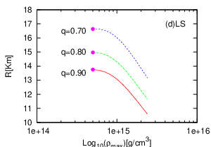
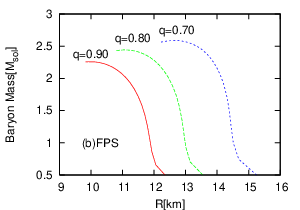
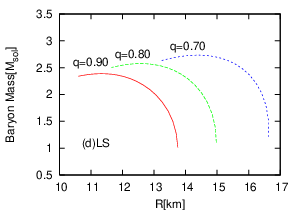
The relation between the physical quantities and the maximum density is an important information and it sometimes helps us to understand the stability of equilibrium configuration. Figure 12 shows maximum density and baryon mass relations in the magnetized rotating stars for the parameters, and for the different EOSs. Long-dashed, short-dashed, and dotted lines represent the relations for , , and , respectively. As a reference relation, we also show one in the spherical configuration as . All sequences reach the mass-shedding limit at . Closed circles correspond to the maximum mass points. As the axis ratios become small, the maximum mass points shift to left, i.e. lower density region. We find that the increase of the maximum mass is up to about twenty percents for the every EOS employed here. In Figure 13, the magnetic fields at the pole are shown as a function of the maximum densities in the same sequences. For the sequences with SLy, FPS, and LS EOSs, the magnetic field at pole is an increasing function of the maximum density for any axis ratio. On the other hand, it is found that only for the sequences with Shen EOS, these exist maximum of the polar magnetic fields around .
How about relations between other physical quantities and the maximum mass ? Figures 14, 15, and 16 are the relations between the rotation periods, equatorial radii, and maximum magnetic field strength with the maximum density. Figure 14 shows the rotation periods are order of millisecond and they decrease with decreasing a value of . This is because these sequences are rotation-dominated type (see Table 4) and more centrifugal force is needed to deform the equilibrium star largely. These features do not depend on the EOSs. From Figure 15, the equatorial radii are order of ten kilometer and decreasing functions of the maximum density. We also find equatorial radii increase with decreasing of . The maximum magnetic field strength are roughly and are increasing functions of maximum density in Figure 16. Note that their values do not depend on because these sequences belong to rotation-dominated type as mentioned above.
As we have already shown, the magnetic field near the rotational axis is like a dipole decaying as for . Now, since we find that is almost insensitive to the values of with fixing the maximum density, should then be proportional to , where is a polar radius. For instance in the sequences with SLy EOS, changes only from to with decreasing of from to . On the other hand, it is found that the change in the equatorial radius is much larger up to about twenty percents for every EOS employed here when changing from to (see Figure 15). For completeness, we finally show relation in Figure 17, where and are baryon mass and equatorial radius, respectively. It is noted that the relation is also valid for the spherical stars, implying that a hierarchy of the stiffness becomes so (Shapiro & Teukolsky 1983).

|

|

|

|

|

|

|

|

|

|

|

|

|

|

|
|

|

|

|

|

|
|

|
|
3.3 Model of Proto-Magnetar
In the previous section, we find that the obtained equilibrium configurations are difficult to be applied for the observed magnetar. Here we decide to construct an equilibrium configuration of a proto-magnetar bearing in mind a hypothesis by Duncan & Thompson 1992 that the magnetars could be originated from the proto-neutron-stars with a surface magnetic field of order and with its rotation period of an order of milliseconds. The models computed here should serve as examples of initial models of the hydrodynamic/evolutionary simulations of the proto-magnetar.
As mentioned in Section 2.2, we can construct a model of proto-magnetar with finite temperature by employing Shen and LS EOSs. In the actual calculation, the maximum density, the parameters associated with magnetic field, axis ratio and entropy per baryon (in unit of Boltzmann’s constant) are fixed as . Here we take the value of the entropy per baryon in the proto-neutron according to Prakash et al. 1997 indicating its distributions to be nearly uniform as a result of the convection.
Results are summarized in Table 5. Note that magnetic field strength at pole is order of . Matter and magnetic field structure of these stars are depicted in Figure 18 and 19. As a result, it is found that the features appearing in the cold magnetized equilibrium configurations above are still valid despite of the incursion of the finite temperature effect on the EOSs. More interestingly, the masses of magnetars are also dependent on the EOSs as shown in Table 5. They are predicted to be as large as for the LS EOS, such neutron stars have never been observed (Lattimer & Prakash 2006). Although we have little observational information about the masses of magnetar so far, our results suggest that we may obtain information about the EOS from the observation of the masses of magnetars.
| h | ||||||
|---|---|---|---|---|---|---|
| Shen | ||||||
| 0.90 | 6.73E+16 | 2.63E+17 | 1.99E+01 | 1.25E+00 | 13.1E+00 | 0.367E+00 |
| LS | ||||||
| 0.90 | 7.32E+16 | 2.80E+17 | 3.01E+01 | 1.06E+00 | 14.9E+00 | 0.326E+00 |

|

|

|

|

|

|

|

|
4 Conclusion
In this paper, we have investigated equilibrium sequences of magnetized rotating stars with four kinds of realistic equations of state (EOSs) of SLy (Douchin & Haensel 2001) et al.), FPS (Pandharipande & Ravenhall 1989), Shen (Shen et al. 1998a), and LS (Lattimer & Swesty 1991). We have employed the Tomimura-Eriguchi scheme to construct the equilibrium configurations.
At first, we have obtained the solution in the regime of Newtonian gravity. Basic properties of the magnetized Newtonian stars are summarized as follows: (1) For the non-rotating sequences, there exist nearly toroidal configurations, , irrespective of the EOSs. The magnetic energy stored in the stars increases with the degree of deformation being larger. (2) For the rotating sequences, we have categorized the sequences with four kinds of EOSs as rotation-dominated (RD) type, magnetic-dominated (MD) one, and nearly toroidal one. As a result, the sequences with softer EOSs of SLy and FPS are found to belong to RD or MD type and the sequences with stiffer EOSs of Shen and LS can belong also to the nearly toroidal one.
(3) We have also focused on the structure of equilibrium configurations. Reflecting the stiffness of EOSs, the density distributions of stars with SLy or FPS EOSs concentrate more at the center than those of the stars with Shen or LS EOSs. The toroidal fields for SLy and FPS EOSs are found to distribute in relatively wider regions in the vicinity of the equatorial plane than for Shen and LS EOSs. The poloidal magnetic fields are also affected by the toroidal fields because poloidal fields are highly distorted where the toroidal fields are strong. Regardless of the difference of the EOSs, a global configuration of magnetic field line is found to be universal, namely the tori of twisted field lines around the symmetry axis inside the star and the untwisted poloidal field lines, which penetrate the stellar surface to continue to the vacuum.
Then, adding the GR correction to the gravity, we have performed the quantitative investigation of the strong magnetized equilibrium stars. As a result, we find that the difference due to the EOSs becomes small because all the employed EOSs become sufficiently stiff for the large maximum density, typically greater than . We have investigated the relation between the baryon mass, the magnetic field at pole, the rotational period, the equatorial radius, and the maximum magnetic field as a function of the maximum density. The typical magnetic fields at pole are about , the periods are about several milliseconds, the radii are about ten kilometers and the maximum magnetic fields are about . The maximum mass is found to be for SLy EOS, for FPS EOS, for Shen EOS and for LS EOS for configurations, respectively. These values are about twenty percents increasing for that of the spherical stars.
Finally, we have computed equilibrium sequences at finite temperature for the Shen and LS EOSs aiming to construct the equilibrium configurations of the proto-magnetars. As a result, it is found that the features appearing in the cold magnetized equilibrium configurations above are still valid despite of the incursion of the finite temperature effect on the EOSs. Since the masses of the proto-magnetars are highly dependent on the EOSs, we have speculated that one may obtain information about the EOSs from the observation of the masses of magnetars.
It is true that our treatment for the general relativistic effect is nothing but a crude approximation. Thus we consider this study as a prelude to a fully general relativistic study, however hoping for the moment that our results could serve as the initial condition for the hydrodynamic evolutionary studies of newly-born magnetars including the microphysical EOSs.
Acknowledgments
We express thanks to S. Yoshida for fruitful discussions and to H. Ono, H. Suzuki, and K. Sumiyoshi for providing us the tabulated table for Lattimer-Swesty EOS. Kiuchi thanks to K. i. Maeda and Kotake to K. Sato for continuing encouragements. Kotake also thanks to S. Yamada and E. Müller for informative discussions. This work was supported in part by the Japan Society for Promotion of Science(JSPS) Research Fellowships (Kiuchi), Grants-in-Aid for the Scientific Research from the Ministry of Education, Science and Culture of Japan (No.1840044 and S19104006).
References
- Akmal et al. (1998) Akmal, A., Pandharipande, V. R., & Ravenhall, D. G. 1998, PRC, 58, 1804
- Baym & Pethick (1979) Baym, G., & Pethick, C. 1979, Ann. Rev. Astron. Astrophys., 17, 415
- Bocquet et al. (1995) Bocquet, M., Bonazzola, S., Gourgoulhon, E., & Novak, J. 1995, A&A, 301, 757
- Bonazzola & Gourgoulhon (1995) Bonazzola, S., & Gourgoulhon, E. 1996, A&A 312, 675
- Braithwaite & Spruit (2004) Braithwaite, J. & Spruit, H. C. 2004, Nature, 431, 819
- Braithwaite & Spruit (2006) Braithwaite, J. & Spruit, H. C. 2006, A&A, 450, 1097
- Chandrasekhar (1956) Chandrasekhar, S., 1956, ApJ 124, 232
- Chandrasekhar & Fermi (1953) Chandrasekhar, S., & Fermi, E. 1953, ApJ 118, 116
- Cowling (1965) Cowling, T. G. 1965, in Stellar Structure, ed. L. H. Allen & D. B. McLaughlin (Chicago: Univ. Chicago Press), 425
- Douchin & Haensel (2001) Douchin, F., & Haensel, P. 2001, A&A, 380, 151
- Duncan & Thompson (1992) Duncan, R. C. & Thompson, C., 1992, ApJ, 392, L9
- Ferrario & Wickramasinghe (2007) Ferrario, L. & Wickramasinghe, D., 2007 Mon. Not. Roy. Astron. Soc. 375, 1009
- Ferraro (1937) Ferraro, V. C. A. 1937, MNRAS 97, 458
- Ferraro (1954) Ferraro, V. C. A. 1954, ApJ 119, 407
- Friedman & Pandharipande (1981) Friedman, B., & Pandharipande, V. R. 1981, Nuclear Physics A, 361, 502
- Glendenning (2001) Glendenning, N. K. 2001, Physics. Rep., 342, 393
- Hachisu (1986) Hachisu, I. 1986, ApJ 61, 479
- Harding & Lai (2006) Harding, A. K., & Lai, D. 2006, Reports of Progress in Physics, 69, 2631
- Hurley (1999) Hurley, K., 1999, arXiv:astro-ph/9912061.
- Ioka (2001) Ioka, K. 2001, MNRAS 327, 639
- Ioka & Sasaki (2003) Ioka, K. & Sasaki, M. 2003, PRD 67, 124026
- Ioka & Sasaki (2004) Ioka, K. & Sasaki, M. 2004, ApJ 600, 296
- Kaspi (2004) Kaspi, V. M. 2004, Young Neutron Stars and Their Environments, 218, 231
- Konno et al. (1999) Konno, K., Obata, T.& Kojima, Y. 1999, A&A, 352, 211
- Kotake et al. (2004) Kotake, K., Sawai, H., Yamada, S., & Sato, K. 2004, ApJ, 608, 391
- Kotake et al. (2004) Kotake, K., Yamada, S., Sato, K., Sumiyoshi, K., Ono, H., & Suzuki, H. 2004 PRD 69, 124004
- Kouveliotou et al. (1998) Kouveliotou, C., et al. 1998, Nature, 393, 235
- Kotake et al. (2006) Kotake, K., Sato, K., & Takahashi, K. 2006, Reports of Progress in Physics, 69, 971
- Lovelace et al. (1986) Lovelace, R. V. E., Mehanian, C. M., & Sulkanen, M. E. 1986, ApJS, 62, 1
- Lattimer & Swesty (1991) Lattimer, J. M., & Douglas Swesty, F. 1991, Nuclear Physics A, 535, 331
- Lattimer & Prakash (2006) Lattimer, J. M. & Prakash, M. 2006 astro-ph/0612440.
- Livne et al. (2007) Livne, E., Dessart, L., Burrows, A., & Meakin, C. A. 2007, ApJS, 170, 187
- Marek et al. (2006) Marek, A., Dimmelmeier, H., Janka, H., Mueller, E., & Buras, R. 2006, A&A, 445, 273
- Markey & Tayler (1973) Markey, P., & Taylar. R. J. 1973 MNRAS, 163, 77
- Markey & Tayler (1974) Markey, P., & Taylar. R. J. 1974 MNRAS, 168, 505
- Mereghetti (1999) Mereghetti, S. arXiv:astro-ph/9911252.
- Mestel (1961) Mestel, L. 1961, MNRAS, 122, 473
- Miketinac (1975) Miketinac, M. J. 1975, Ap&SS, 35, 349
- Moiseenko et al. (2006) Moiseenko, S. G., Bisnovatyi-Kogan, G. S., & Ardeljan, N. V. 2006, MNRAS, 370, 501
- Monaghan (1965) Monaghan, J. J. 1965, MNRAS, 131, 105
- Monaghan (1966) Monaghan, J. J. 1966, MNRAS, 134, 275
- Morrison et al. (2004) Morrison, I. A., Baumgarte, T. W., & Shapiro, S. L. 2004, ApJ, 610, 941
- Nozawa et al. (1998) Nozawa, T., Stergioulas, N., Gourgoulhon, E., & Eriguchi, Y. 1998, A&A Sup. Ser., 132, 431
- Obergaulinger et al. (2006) Obergaulinger, M., Aloy, M. A., Müller, E. 2006, A&A, 450, 1107
- Oppenhimer & Volkoff (1939) Oppenheimer, J. R., & Volkoff, G. 1939, Phys. Rev., 55, 374
- Ostriker & Hartwick (1968) Ostriker, J. P. & Hartwick, F. D. A. 1968, ApJ, 153, 797
- Ostriker & Mark (1968) Ostriker, J. P. & Mark, J. W-K. 1968, ApJ, 151, 1075
- Pandharipande & Ravenhall (1989) Pandharipande, V. R., & Ravenhall, D. G. 1989, NATO ASIB Proc. 205: Nuclear Matter and Heavy Ion Collisions, 103
- Prakash et al. (1997) Prakash, M., Bombaci, I., Prakash, M., Ellis, P. J., Lattimer, J. M., and Knorren, R. 1997, Phys. Rept. 280, 1
- Prendergast (1956) Prendergast, K. H. 1956, ApJ, 123, 498
- Rampp & Janka (2002) Rampp, M., & Janka, H.-T. 2002, A&A, 396, 361
- Roberts (1955) Roberts, P. H. 1955, ApJ, 122, 508
- Roxburgh (1966) Roxburgh, I. W. 1966, MNRAS, 132, 347
- Sawai et al. (2005) Sawai, H., Kotake, K., & Yamada, S. 2005 ApJ 631, 446
- Shapiro & Teukolsky (1983) Shapiro, S. L., & Teukolsky, S. A. 1983, Research supported by the National Science Foundation. New York, Wiley-Interscience, 1983, 663 p.,
- Shibata et al. (2005) Shibata, M., Taniguchi, K., & Uryu, K. 2005 PRD 71, 084021
- Shen et al. (1998a) Shen, H., Toki, H., Oyamatsu, K., Sumiyoshi, K. 1998, Nuclear Physics, A637, 43, 109, 301
- Shen et al. (1998b) Shen, H., Toki, H., Oyamatsu, K., & Sumiyoshi, K. 1998, Progress of Theoretical Physics, 100, 1013
- Shibata et al. (2006) Shibata, M., Liu, Y. T., Shapiro, S. L., & Stephens, B. C. 2006 PRD 74, 104026
- Sumiyoshi et al. (2005) Sumiyoshi, K., Yamada, S., Suzuki, H., Shen, H., Chiba, S., & Toki, H. 2005, ApJ, 629, 922
- Takiwaki et al. (2004) Takiwaki, T., Kotake, K., Nagataki, S., & Sato, K. 2004, ApJ, 616, 1086
- Thompson & Duncan (1993) Thompson, C. & Duncan, R. C. 1993, ApJ, 408, 194
- Thompson & Duncan (1995) Thompson, C. & Duncan, R. C. 1995, Mon. Not. Roy. Astron. Soc. 275, 255
- Thompson & Duncan (1996) Thompson, C. & Duncan, R. C. 1996, ApJ 473, 322
- Tomimura & Eriguchi (2005) Tomiumra, Y. & Eriguchi, Y., 2005 MNRAS, 359, 1117
- Watts (2006) Watts, A. 2006, 36th COSPAR Scientific Assembly, 36, 168
- Wiringa et al. (1988) Wiringa, R. B., Fiks, V., & Fabrocini, A. 1988, PRC, 38, 1010
- Woltjer (1960) Woltjer, L. 1960, ApJ, 131, 227
- Woods & Thompson (2004) Woods, P. M. & Thompson, C. 2004, arXiv:astro-ph/0406133.
- Wright (1973) Wright, G. A. E. 1973, MNRAS, 162, 339
- Yamada & Sawai (2004) Yamada, S., & Sawai, H. 2004, ApJ, 608, 907
- Yoshida & Eriguchi (2006) Yoshida, S. & Eriguchi, Y. 2006, ApJS, 164, 156
- Yoshida et al. (2006) Yoshida, S., Yoshida, S., & Eriguchi, Y. 2006, ApJ, 651, 462
Appendix A Code Test
To check our code ability, we calculate the same sequences shown in Yoshida & Eriguchi 2006 with polytropic equations of state. We actually obtain two kinds of sequences, non-rotating sequence and rotating-sequence. In Table 6, some physical quantities of the non-rotating sequence with the polytropic index , and (see equation (25), (26)) are shown. For the axis ratio , the upper row corresponds to the result by Yoshida & Eriguchi 2006 and the down one do to our result. Table 7 is a result of the rotating sequence with polytropic index , , and . In all sequences, the relative errors for the each quantities with Yoshida & Eriguchi 2006’s result are less than one percent and VC is . Therefore, we confirm that our code works well.
| q | VC | |||||||
|---|---|---|---|---|---|---|---|---|
| 0.98 | 0.0050 | 0.332 | 7.310E-4 | 0.140 | -6.348E-3 | 5.276E-3 | 0.078 | |
| 0.0050 | 0.332 | 7.310E-4 | 0.140 | -6.348E-3 | 5.276E-3 | 0.078 | 2.55E-4 | |
| 0.90 | 0.0275 | 0.324 | 7.922E-4 | 0.299 | -7.163E-3 | 5.303E-2 | 0.082 | |
| 0.0275 | 0.324 | 7.922E-4 | 0.299 | -7.163E-3 | 5.303E-2 | 0.082 | 2.54E-4 | |
| 0.80 | 0.0635 | 0.312 | 9.004E-4 | 0.408 | -8.526E-3 | 5.335E-2 | 0.088 | |
| 0.0635 | 0.312 | 9.004E-4 | 0.408 | -8.526E-3 | 5.335E-2 | 0.088 | 2.50E-4 | |
| 0.70 | 0.1131 | 0.296 | 1.097E-3 | 0.476 | -1.064E-2 | 5.400E-3 | 0.099 | |
| 0.1131 | 0.296 | 1.097E-3 | 0.476 | -1.064E-2 | 5.400E-3 | 0.099 | 2.37E-4 | |
| 0.60 | 0.1856 | 0.272 | 1.560E-3 | 0.501 | -1.456E-2 | 5.576E-3 | 0.121 | |
| 0.1856 | 0.272 | 1.560E-3 | 0.501 | -1.456E-2 | 5.575E-3 | 0.121 | 2.07E-4 | |
| 0.50 | 0.3044 | 0.232 | 4.087E-3 | 0.447 | -2.721E-2 | 6.524E-3 | 0.211 | |
| 0.3042 | 0.232 | 4.079E-3 | 0.447 | -2.718E-2 | 6.520E-3 | 0.210 | 1.21E-4 | |
| 0.40 | 0.4087 | 0.197 | 7.624E-3 | 0.279 | -3.845E-2 | 6.188E-3 | 0.320 | |
| 0.4086 | 0.197 | 7.637E-3 | 0.279 | -3.849E-2 | 6.190E-3 | 0.321 | 6.59E-6 | |
| 0.30 | 0.4219 | 0.193 | 4.626E-3 | 0.247 | -3.022E-2 | 4.713E-3 | 0.254 | |
| 0.4218 | 0.193 | 4.638E-3 | 0.247 | -3.026E-2 | 4.716E-3 | 0.254 | 8.43E-6 | |
| 0.20 | 0.4287 | 0.190 | 3.434E-3 | 0.237 | -2.635E-2 | 4.003E-3 | 0.220 | |
| 0.4287 | 0.190 | 3.453E-3 | 0.237 | -2.643E-2 | 4.009E-3 | 0.221 | 3.12E-6 | |
| 0.10 | 0.4326 | 0.189 | 2.900E-3 | 0.233 | -2.443E-2 | 3.648E-3 | 0.203 | |
| 0.4326 | 0.189 | 2.926E-3 | 0.233 | -2.454E-2 | 3.658E-3 | 0.204 | 1.52E-5 | |
| 0.01 | 0.4338 | 0.189 | 2.743E-3 | 0.233 | -2.384E-2 | 3.539E-3 | 0.197 | |
| 0.4338 | 0.189 | 2.771E-3 | 0.232 | -2.396E-2 | 3.550E-3 | 0.198 | 1.96E-5 |
| q | VC | ||||||||
|---|---|---|---|---|---|---|---|---|---|
| - | - | - | - | - | - | - | - | - | |
| 0.98 | 2.75E-3 | 0.331 | 2.04E-3 | 2.68E-1 | 1.50E-3 | -0.181 | 8.61E-2 | 2.24 | |
| 2.74E-3 | 0.331 | 2.04E-3 | 2.68E-1 | 1.50E-3 | -0.181 | 8.61E-2 | 2.24 | 2.19E-4 | |
| 0.90 | 2.88E-3 | 0.317 | 2.37E-2 | 2.31E-1 | 1.64E-2 | -0.175 | 7.78E-2 | 2.05 | |
| 2.89E-3 | 0.317 | 2.37E-2 | 2.31E-1 | 1.64E-2 | -0.175 | 7.77E-2 | 2.05 | 1.37E-4 | |
| 0.80 | 3.10E-3 | 0.297 | 5.33E-2 | 1.86E-1 | 3.40E-2 | -0.166 | 6.71E-2 | 1.80 | |
| 3.10E-3 | 0.297 | 5.33E-2 | 1.86E-1 | 3.40E-2 | -0.166 | 6.71E-2 | 1.80 | 1.25E-4 | |
| 0.70 | 3.37E-3 | 0.275 | 8.60E-2 | 1.44E-1 | 4.98E-2 | -0.155 | 5.63E-2 | 1.55 | |
| 3.37E-3 | 0.274 | 8.60E-2 | 1.44E-1 | 4.98E-2 | -0.155 | 5.63E-2 | 1.55 | 1.35E-4 | |
| 0.60 | 3.72E-3 | 0.251 | 1.22E-1 | 1.04E-1 | 6.29E-2 | -0.141 | 4.55E-2 | 1.29 | |
| 3.73E-3 | 0.251 | 1.22E-1 | 1.04E-1 | 6.29E-2 | -0.141 | 4.55E-2 | 1.29 | 1.22E-4 | |
| 0.50 | 4.21E-3 | 0.225 | 1.61E-1 | 6.75E-2 | 7.19E-2 | -0.123 | 3.46E-2 | 1.01 | |
| 4.22E-3 | 0.225 | 1.61E-1 | 6.76E-2 | 7.19E-2 | -0.123 | 3.46E-2 | 1.01 | 8.79E-5 | |
| 0.43 | 3.64E-3 | 0.210 | 1.83E-1 | 4.06E-2 | 7.46E-2 | -0.101 | 2.67E-2 | 0.750 | |
| 3.67E-3 | 0.210 | 1.84E-1 | 4.07E-2 | 7.46E-2 | -0.102 | 2.67E-2 | 0.750 | 9.53E-5 | |
| MS | - | - | - | - | - | - | - | - | - |
Appendix B General Relativistic Correction
We start from the metric of spherical symmetry space time,
| (48) |
Matter is assumed as a perfect fluid, thus the energy momentum tensor is
| (49) |
where , , and are a density, specific internal energy, and pressure. TOV equation (Oppenhimer & Volkoff 1939) is
| (50) | |||
| (51) |
where is relativistic enthalpy and is mass function defined as
Equation for the potential is
| (52) |
This potential, of course, reduces to the gravitational potential in the Newtonian limit. To make clear a general relativistic contribution in the potential, we perform the Taylor expansion of equation (52) with respect to , which is guaranteed to be small than unity in star. Result is written in the form,
| (53) |
Note that the first term is a contribution from Newtonian gravitational potential. So, we define a general relativistic correction in the potential as . Boundary condition is derived from a requirement that the outer vacuum space time is equivalent to the Schwarzschild space time,
| (54) |
where and are radius and ADM mass of the star. From the Taylor expansion with respect to , the boundary condition for the general relativistic correction term is derived. As a result, is expressed in an integral form,
| (55) |
This spherically symmetric effective potential is also applied in our 2D axisymmetric configuration code, where we first compute angular averages of the relevant hydrodynamical variables. These are then used to calculate the spherical general correction term in equation (55). Consequently, we modify the 2D Newtonian potential to obtain the two dimensional general relativistic potential
| (56) |
The method shown in Marek et al. 2006 has an ambiguity in definition of potential and imposes boundary condition of their potential at infinity. However, in our method the general relativistic correction in the potential is explicitly written down and its boundary condition is imposed at the stellar surface. So, the two method is a little bit different. Verification of our method is shown in the last in this appendix. Subsequently, we focus on the Bernoulli equation, which is ordinary used to obtain axisymmetric configuration (e.g. (21)). Under the metric form (50), four velocity is given by
| (57) |
The relativistic Bernoulli equation with spherically symmetric is also written as
| (58) |
where and C are relativistic enthalpy, integral constant, respectively. Combining equations (57)-(58), we find
| (59) |
Finally we modify the Bernoulli equation of magnetized rotating case as
| (60) |
Note that this treatment may be speculation. To verify our treatment, we calculate spherical symmetric stars with four kinds of EOS in both 1D TOV code and 2D axisymmetric code. Relations of mass, both ADM and baryon mass, with central density in these stars are displayed in Figure 20. We confirm our treatment works well.

|

|

|

|