On the Distortion of the Eigenvalue Spectrum in MIMO Amplify-and-Forward Multi-Hop Channels

We consider coherent wireless multiple-input-multiple-output (MIMO) communication between $n_{\mathrm{s}}$ non-cooperating source antennas and $n_{\mathrm{d}}$ fully cooperating destination antennas. In this paper it is assumed that the source antennas are either far apart or shadowed from the destination antennas. The installation of intermediate nodes that relay the source signals to the destination (multi-hop) is well known for being an efficient means for improving the energy-efficiency of the communication system in this case. In the resulting network, the signals traverse $L$ clusters containing $k$ relay antennas each, before they reach the destination. Generally, signals transmitted by the source antennas might not only be received by the immediately succeeding cluster of relay antennas, but possibly also by clusters that are farther away or by the destination. While such receptions could well be exploited for achieving higher transmission rates, we assume them to be strongly attenuated and ignore them in this paper.

In the most basic MIMO multi-hop network architecture, the relay antennas in the clusters do not cooperate. Since non-cooperative decoding of the interfering source signals at the individual relay antennas drastically reduces the achievable rate in the network, a simple amplify-and-forward operation becomes the relaying strategy of choice. That is, at each antenna a scaling of the received signals by a constant is performed before the retransmission. While this approach is cheap in terms of computational complexity, and also does not require any channel-state information at the relay nodes, it clearly suffers from noise accumulation. This basic network has been studied extensively by Borade, Zheng and Gallager for independent identically distributed (i.i.d.) Rayleigh fading channel matrices. In references [1, 2] they showed for $n\triangleq n_{\mathrm{s}}=n_{\mathrm{d}}=k$ that all $n$ spatial degrees of freedom are available in this network for a fixed $L$ at high signal-to-noise ratio (SNR). More generally, they also showed that all degrees of freedom are available, if $L$ as a function of the SNR fulfills $\lim_{\mathsf{snr}\rightarrow\infty}L(\mathsf{snr})/\log\mathsf{snr}=0$.

While this result gives a design criterion how the SNR should be increased with the number of hops in the network, it does not give any insights into the eigenvalue distribution of the product of random matrices $\mathbf{C}$ specifying the mutual information between input and output of the vector channel. For fixed $L$, only recently this eigenvalue distribution has been characterized in the large antenna limit [3]. Based on a theorem from large random matrix theory [4], the authors showed that it converges to a deterministic function, and gave a recursive formula for the corresponding Stieltjes transform. Moreover, the reference reports that the asymptotic eigenvalue distribution of $\mathbf{C}$, which is in fact the product of the signal covariance matrix $\mathbf{R}_{s}$ and inverse noise covariance matrix $\mathbf{R}_{n}^{-1}$ at the destination, approaches the Marčenko-Pastur law in the large dimensions limit for $\beta_{r}\triangleq k/n_{\mathrm{d}}\rightarrow\infty$, but $\beta_{s}\triangleq n_{\mathrm{s}}/n_{\mathrm{d}}$ and $L$ fixed. Since the Marčenko-Pastur law is also the limiting eigenvalue distribution of the classical point-to-point MIMO channel, this means that up to a noise penalty and a pre-log factor the point-to-point capacity is approached in this case.

By considering the limiting eigenvalue distributions of the signal and noise covariance matrices separately, we are able to generalize this result for the case $L\rightarrow\infty$ in this paper. In essence, we show that $\beta_{r}$ needs to grow at least linearly with $L$ in order to sustain a non-zero fraction of the spatial degrees of freedom in the system, i.e., linear capacity scaling in $\min\{n_{\mathrm{s}},n_{\mathrm{d}}\}$. Moreover, when the scaling is faster than linear, the limiting eigenvalue distribution of $\mathbf{C}$ is given by the Marčenko-Pastur law. That is, we are able exploit the spatial degrees of freedom without increasing the SNR at the receiver at the expense of employing more relay antennas. Returning to the result by Borade et al., where degrees of freedom are sustained by increasing the SNR, according to our result the number of relays per layer can be seen as a second resource besides the transmit power for compensating the capacity loss in the multi-hop network.

Another contribution of this paper lies in bridging the gap between the results obtained by Müller in reference [5] on the one hand and by Morgenshtern and Bölcskei in references [6, 7] on the other hand. In the first reference, it is shown in the large dimensions limit that almost all singular values of a product of independent random matrices fulfilling the conditions needed for the Marčenko-Pastur law go to zero as the number of multipliers grows large, while the aspect ratios of the matrices are kept finite. This implies that almost all spatial degrees of freedom in a MIMO amplify-and-forward multi-hop network as described above vanish as $L$ goes to infinity. On the other hand, [6, 7] were the first papers which proved in the large dimensions limit (for $L=1$) that the capacity of a point-to-point MIMO link is approached up to a noise penalty and a pre-log factor, if $\beta_{r}\rightarrow\infty$ and $\beta_{s}$ is kept fixed. In [8] the same result had been proven for the less general case that $n_{\mathrm{s}}$ and $n_{\mathrm{d}}$ are fixed and $k\rightarrow\infty$. The mechanisms discovered in these papers apparently act as antipodal forces with respect to the limiting eigenvalue distributions of products of random matrices. While increasing the number of hops distorts this distribution in an undesired fashion, increasing the ratio between the number of relays and destination antennas allows for recovering the original distribution corresponding to a point-to-point channel. In this paper, we answer the question how these two effects can be balanced, i.e., how fast must $\beta_{r}$ grow with $L$ in order to sustain a non-zero fraction of spatial degrees of freedom as $L$ grows without bounds.

The superscripts ^H and ^∗ stand for conjugate transpose and complex conjugate, respectively. $\textsf{E}_{A}$ denotes the expectation operator with respect to the random variable $A$. $\det(\mathbf{A})$, $\mathrm{Tr}(\mathbf{A})$ and $\lambda_{i}\{\mathbf{A}\}$ stand for determinant, trace and the $i$th eigenvalue of the matrix $\mathbf{A}$. $a(i)$ is the $i$th element of the vector $\mathbf{a}$. Throughout the paper all logarithms, unless specified otherwise, are to the base $e$. $\|\mathbf{a}\|$ denotes the Euclidean norm of the vector $\mathbf{a}$, $\|\mathbf{A}\|_{\mathrm{Tr}}$ the Trace norm of the matrix $\mathbf{A}$. By $\textsf{Pr}[A]$ we denote the probability of the event $A$.

Furthermore, we use the standard ${\cal O}(\cdot),\Omega(\cdot),\Theta(\cdot)$ notations for characterizing the asymptotic behavior of some function $f(\cdot)$ according to

Finally, we define the function $1\{x\}$ to be 1 if $x$ is true and zero otherwise. $\delta(x)$ and $\sigma(x)$ denote Dirac delta and Heaviside step function, respectively.

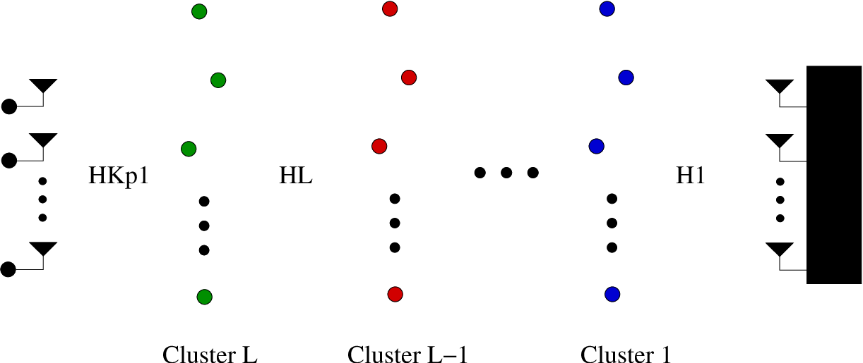
We label the clusters of relay antennas by $\mathcal{C}_{1},\ldots,\mathcal{C}_{L}$. Cluster $\mathcal{C}_{1}$ denotes the one next to the destination, $\mathcal{C}_{L}$ the one next to the sources (refer to Fig. 1). We assume the $L+1$ single hop channels between sources, relay clusters and destinations to be frequency-flat fading over the bandwidth of interest, and divide the transmission into $L+1$ time slots. In time slot $T=1$ the sources transmit to $\mathcal{C}_{L}$. The transmission is described by the transmit vector $\mathbf{s}\in\mathbb{C}^{n_{\mathrm{s}}}$, the matrix $\mathbf{H}_{L+1}\in\mathbb{C}^{k\times n_{\mathrm{s}}}$, representing the vector channel between sources and $\mathcal{C}_{L}$, the vector $\mathbf{n}_{L}\in\mathbb{C}^{k}$, representing the receiver front-end noise introduced in $\mathcal{C}_{L}$, the receive vector $\mathbf{y}_{L}\in\mathbb{C}^{k}$ and the linear mapping

Here and also in the subsequent equations, the $i$th elements of the transmit, receive and noise vectors correspond to the $i$th antenna in the respective network stage.

The time slots $T=\{2,\ldots,L\}$ are used for relaying the signals from cluster to cluster. In time slot $T$ the relay antennas in $\mathcal{C}_{L-T+2}$ transmit scaled versions of the signals received in time slot $T-1$ to $\mathcal{C}_{L-T+1}$. That is, with $l=L-T+2$ the transmit vector of the $l$th relay cluster $\mathbf{r}_{l}\in\mathbb{C}^{k}$ is computed from the respective receive vector $\mathbf{y}_{l}\in\mathbb{C}^{k}$ according to

where $\mathbf{\alpha}_{l}\in\mathbb{R}$ is a cluster specific constant of proportionality specifying the ratio between receive and transmit power. The transmission in time slot $T$ is then described by

Here, $\mathbf{H}_{l}\in\mathbb{C}^{k\times k}$ represents the channel between $\mathcal{C}_{l}$ and $\mathcal{C}_{l-1}$, $\mathbf{n}_{l-1}\in\mathbb{C}^{k}$ the receiver front-end noise introduced in $\mathcal{C}_{l-1}$, and $\mathbf{y}_{l-1}\in\mathbb{C}^{k}$ is the corresponding receive vector. Thus, the signals traverse one hop per time slot. In time slot $T=L+1$, $\mathcal{C}_{1}$ finally forwards its received signals to the destination. Again, the transmit vector is computed according to $\mathbf{r}_{1}=\sqrt{\frac{\alpha_{1}}{k}}\mathbf{y}_{1}$. Denoting the matrix representing the channel between $\mathcal{C}_{1}$ and the destination by $\mathbf{H}_{1}$, the vector representing the receiver front-end noise at the destination by $\mathbf{n}_{d}\in\mathbb{C}^{n_{\mathrm{d}}}$ and the receive vector by $\mathbf{y}\in\mathbb{C}^{n_{\mathrm{d}}}$ this transmission is described by

Putting everything together, the input-output relation of the channel as seen from source to destination antennas over $L+1$ time slots can be written as

We model the entries of all noise vectors as zero-mean circular symmetric complex Gaussian random variables of unit-variance that are white both in space and time. The channel matrices are independent and their elements are assumed to be i.i.d. zero-mean random variables of unit-variance. Moreover, we impose the per antenna power constraints $\textsf{E}[s(i)s(i)^{*}]=P/n_{\mathrm{s}}$ and $\textsf{E}[r_{l}(i)r_{l}(i)^{*}]=P/k$ for $l=\{1,\ldots,L\}$. The relay antenna power constraints are fulfilled, if the scaling factors $\alpha_{i}$ satisfy $\alpha\triangleq\alpha_{1}=\ldots=\alpha_{L}=P/(P+1)$.

While full cooperation and the presence of full channel-state information is assumed at the destination antennas, source and relay antennas do not cooperate and also do not possess any channel-state information. Under these assumptions, the ergodic mutual information $I(\mathbf{s};\mathbf{y})$ is maximized, when the entries of $\mathbf{s}$ are zero-mean circularly symmetric complex Gaussian random variables of variance $P/n_{\mathrm{s}}$ that are white over both space and time [9]. For this input distribution, $I(\mathbf{s};\mathbf{y})$ is fully characterized by the joint probability distribution of the eigenvalues of the product $\mathbf{C}=\mathbf{R}_{s}\mathbf{R}_{n}^{-1}$, where $\mathbf{R}_{s}\in\mathbb{C}^{n_{\mathrm{d}}\times n_{\mathrm{d}}}$ and $\mathbf{R}_{n}\in\mathbb{C}^{n_{\mathrm{d}}\times n_{\mathrm{d}}}$ denote the signal and noise covariance matrices at the destination of the multi-hop channel. These covariance matrices are given by

We define the the empirical eigenvalue distribution (EED) of the matrix $\mathbf{A}$ as

With this notation the ergodic capacity of the multi-hop channel in nats per channel use is obtained as

Note that the pre-log factor $(L+1)^{-1}$ accounting for the use of $L+1$ time slots can be lowered by initiating the next source antenna transmission after $L_{0}<L$ time slots. From a practical perspective $L_{0}$ needs to be chosen large enough, such that the interference imposed on the previously transmitted signal is negligible. It is important to have this fact in mind whenever we take the limit $L\rightarrow\infty$, which formally drives the ergodic capacity to zero. In this paper we are interested in the scaling of the capacity in the number of source and destination antennas. Accordingly, we focus on the case where both these quantities grow large. From [3] we know that $F_{\mathbf{C}}^{(n)}(x)$ converges almost surely (a.s.) to some asymptotic distribution $F_{\mathbf{C}}(x)$, when $n_{\mathrm{s}}\rightarrow\infty$, $n_{\mathrm{d}}\rightarrow\infty$ and $k\rightarrow\infty$, but the ratios $\beta_{s}=n_{\mathrm{s}}/n_{\mathrm{d}}$ and $\beta_{r}=k/n_{\mathrm{d}}$ are fixed. Here, we mean by the convergence of an EED $F_{\mathbf{A}}^{(n)}(x)$ to some deterministic function $F_{\mathbf{A}}(x)$ that

We will refer to the density $f_{\mathbf{A}}(x)=\frac{d}{dx}F_{\mathbf{A}}(x)$ as the limiting spectral measure (LSM) subsequently.

Returning to the capacity expression (2), we can infer that for $n_{\mathrm{s}}\rightarrow\infty$, $n_{\mathrm{d}}\rightarrow\infty$ and $k\rightarrow\infty$, and $\beta_{s}$ and $\beta_{r}$ fixed, $C$ converges to the quantity $C_{\infty}$ defined as

We briefly repeat some preliminaries from the theory of large random matrices subsequently.

We formalize our result in the subsequent theorem. It is important to note that taking the limits in the LSM of a random matrix means that the dimensions of this matrix are already taken to infinity. For the case at hand that is, we first take the limits $n_{\mathrm{s}}\rightarrow\infty$, $n_{\mathrm{d}}\rightarrow\infty$ and $k\rightarrow\infty$, and then take the limits $L\rightarrow\infty$ and $\beta_{r}\rightarrow\infty$. Whenever we take the limits $L\rightarrow\infty$ and $\beta_{r}\rightarrow\infty$ in an LSM of some random matrix $\mathbf{A}$ or in the corresponding Stieltjes transform, we denote the asymptotic expressions by

This section provides the proof of Theorem 2. We start out with the lemma below, which will allow for inferring a corollary to Theorem 1. This corollary is the key to the proof of Theorem 2 in this section. In order not to interrupt the logical flow of the section two rather technical lemmas required for the proof of Theorem 2, are stated and proven in the Appendix of this paper.

Analogously, if $g(\kappa)\in\Omega(\kappa^{1+\varepsilon})$, there exists some $M>0$, such that the exponent in (12) can be lower bounded according to

Evaluating (13) for $\gamma=1+\varepsilon$ renders the upper bound infinite, which establishes that both the LHS of (15) and (12) grow without bound in this case.

Finally, if $g(\kappa)\in\Theta(\kappa)$, there exist constants $M_{1}$ and $M_{2}$, fulfilling $M_{2}\geq M_{1}>0$, such that according to (13) evaluated for $\gamma=1$ the exponent in (12) is sandwiched between

which establishes the second part of the lemma. $\blacksquare$

The part of the corollary related to the $\mathbf{R}_{n,l}$’s is actually stated more generally than needed in this paper. In fact, we are only going to use that for some fixed positive integer $L_{\mathrm{t}}<L$, the LSMs of the $\mathbf{R}_{n,l}$’s, where $l\in\{1,\ldots,L_{\mathrm{t}}\}$, are given by a Dirac delta at one, i.e., have the Stieltjes transform (18), when $\beta_{r}\rightarrow\infty$, independently of the scaling of $\beta_{r}$ in $L$. This is trivially guaranteed by the corollary, since when $L_{\mathrm{t}}$ is constant, $L_{\mathrm{t}}\in\mathcal{O}(\beta_{r}^{1-\varepsilon})$ is fulfilled naturally as $\beta_{r}\rightarrow\infty$.

For the case $L\in\Theta(\beta_{r})$ we know from Lemma 1 that $\Psi_{s}(\beta_{r},L)=e^{d(sG_{\tilde{\mathbf{R}}_{s}}^{(\infty)}(s)-1)}$ in the limit of interest for some $d>0$. Thus (6) simplifies to

There exists no closed form solution to this implicit equation. However, it is easily verified that $G_{\tilde{\mathbf{R}}_{s}}^{(\infty)}=s^{-1}$ does not satisfy (21).

For (18), we obtain the equation for the Stieltjes transform corresponding to the LSM of $\mathbf{R}_{n,l}$, where $l\in\{1,\ldots,L\}$, from (6) with $N=l$, $\beta_{0}=1$ and $\beta_{n}=\beta_{r}$ for $n\in\{1,\ldots,l\}$ as

Let’s consider the case $l=L$ first. If $L\in\mathcal{O}\left(\beta_{r}^{1-\varepsilon}\right)$, $\Psi_{n}(\beta_{r},l)$ converges to one in the limit $k\rightarrow\infty$ and $L\rightarrow\infty$ by Lemma 1. Therefore, in this limit (22) simplifies to

The solution to (23) is given by $G_{\mathbf{R}_{n,L}}^{(\infty)}(s)=(s+1)^{-1}$. The same is trivially true for all $\mathbf{R}_{n,l}$ with $l<L$, since whenever $L\in\mathcal{O}\left(\beta_{r}^{1-\varepsilon}\right)$, this implies that also $l\in\mathcal{O}(\beta_{r}^{1-\varepsilon})$. $\blacksquare$

We are now ready to prove Theorem 2. Besides the above corollary, we use the Lemmas 2 & 3, which are stated and proven in the Appendix of this paper.

In a next step we can choose $L$ (and thus $\beta_{r}$) large enough such that the accumulated noise power originating from the relays $1,\ldots,L_{\mathrm{t}}-1$ becomes sufficiently white. This means, for the fixed $L_{\mathrm{t}}$ and the same $\varepsilon$ as defined above there exist $L_{0}>L_{\mathrm{t}}$ and $n_{0}^{(2)}(L,L_{\mathrm{t}})$, such that a.s. for all $L\geq L_{0}$ and for all $n\geq n_{0}^{(2)}(L,L_{\mathrm{t}})$

The proof is similar to the one above:

Again, the first identity is a standard identity for a geometric series. In this case the convergence of the arguments of the $\max(\cdot)$ function is guaranteed by Corollary 1 and Lemma 2 (refer to Appendix): Corollary 1 tells us that the LSMs of all the $\frac{1}{k^{l}}\mathbf{H}_{1}\cdots\mathbf{H}_{l}\mathbf{H}_{l}^{\mathrm{H}}\cdots\mathbf{H}_{1}^{\mathrm{H}}$’s, where $l\in\{1,\ldots,L_{\mathrm{t}}-1\}$, converge to a Dirac at one in the limit under consideration. Knowing this, Lemma 2 guarantees us that the respective Trace norms go to zero. Thus, there exist $L_{0}$ and $n_{0}^{(2)}(L,L_{\mathrm{t}})$, such that a.s. the maximum of the $L_{\mathrm{t}}-1$ terms is small enough to make (26) smaller than $\varepsilon/3$ for all $L>L_{0}$ and $n\geq n_{0}^{(2)}(L,L_{\mathrm{t}})$.

References

• [1] S. Borade, L. Zheng, and R. Gallager, “Maximizing degrees of freedom in wireless networks,” in Proc. Allerton Conf. Commun., Contr., and Computing, Monticello, IL, Oct. 2003.
• [2] ——, “Amplify and forward in wireless relay networks: Rate, diversity and network size,” IEEE Trans. Inform. Theory, Special Issue on Relaying and Cooperation in Communication Networks, Oct. 2007, to appear.
• [3] S. Yeh and O. Lévêque, “Asymptotic capacity of multi-level amplify-and-forward relay networks,” in Proc. IEEE Int. Symposium on Inf. Theory, Nice, France, June 2007.
• [4] J. Silverstein, “Strong covergence of the empirical distribution of eigenvalues of large dimensional random matrices,” Journal of Multivariate Anal., vol. 55, pp. 331––339, Nov. 1995.
• [5] R. R. Müller, “On the asymptotic eigenvalue distribution of concatenated vector-valued fading channels,” IEEE Trans. Inform. Theory, vol. 48, no. 7, pp. 2086–2091, July 2002.
• [6] V. I. Morgenshtern and H. Bölcskei, “Random matrix analysis of large relay networks,” in Proc. Allerton Conf. Commun., Contr., and Computing, Monticello, IL, Sept. 2006.
• [7] ——, “Crystallization in large wireless networks,” IEEE Trans. Inform. Theory, Special Issue on Relaying and Cooperation in Communication Networks, Oct. 2007, to appear.
• [8] H. Bölcskei, N. U. Nabar, O. Oyman, and A. J. Paulraj, “Capacity scaling laws in MIMO relay networks,” IEEE Trans. Wireless Commun., vol. 5, no. 6, pp. 1433–1444, June 2006.
• [9] I. E. Telatar, “Capacity of multi-antenna Gaussian channels,” European Transactions on Telecommunications, vol. 10, no. 6, pp. 585–595, Nov. 1999.
• [10] V. A. Marcenko and L. A. Pastur, “Distributions of eigenvalues for some sets of random matrices,” Math. USSR-Sbornik, vol. 1, pp. 457––483, 1967.
• [11] Z. D. Bai, “Methodologies in spectral analysis of large dimensional random matrices,” Statistica Sinica, vol. 9, pp. 611–677, 1999.
• [12] D. Voiculescu, “Multiplication of certain non-commuting random variables,” Journal of Operator Theory, vol. 18, pp. 223–235, 1987.
• [13] R. R. Müller, “Random matrices, free probability and the replica method,” in Proc. of European Signal Processing Conference (Eusipco), Vienna, Austria, Sept. 2004.
• [14] S. Verdú, “Large random matrices and wireless communications,” in MRSI Information Theory Workshop, Berkeley, CA, Feb./Mar. 2002.
• [15] A. M. Tulino and S. Verdú, Random matrix theory and wireless communications. Now Publishers Inc., 2004.
Refer to caption
Fig. 1: nsn_{\mathrm{s}} non-cooperating source antennas transmit to a destination terminal with ndn_{\mathrm{d}} antennas via LL clusters of kk non-cooperating relay antennas.
Fig. 2: Normalized capacity C0C_{0} versus the number of relay clusters LL as obtained through Monte Carlo simulations. The number of source and destination antennas is n=10n=10. The SNR at the destination is 10 dB. The number of relays per cluster kk evolves according to k=n⋅Lγk=n\cdot L^{\gamma}. The dashed curve shows the normalized point-to-point MIMO capacity as a reference.
Fig. 3: Normalized capacity C0C_{0} versus the number of relay clusters LL as obtained through Monte Carlo simulations. The number of source and destination antennas is n=10n=10. The SNR at the destination is 10 dB. The number of relays per cluster kk evolves according to k=n⋅Lγk=n\cdot L^{\gamma}. The dashed curve shows the normalized point-to-point MIMO capacity as a reference.