Stability and nonlinear adjustment of vortices in Keplerian flows
Abstract
Aims. We investigate the stability, nonlinear development and equilibrium structure of vortices in a background shearing Keplerian flow
Methods. We make use of high-resolution global two-dimensional compressible hydrodynamic simulations. We introduce the concept of nonlinear adjustment to describe the transition of unbalanced vortical fields to a long-lived configuration.
Results. We discuss the conditions under which vortical perturbations evolve into long-lived persistent structures and we describe the properties of these equilibrium vortices. The properties of equilibrium vortices appear to be independent from the initial conditions and depend only on the local disk parameters. In particular we find that the ratio of the vortex size to the local disk scale height increases with the decrease of the sound speed, reaching values well above the unity. The process of spiral density wave generation by the vortex, discussed in our previous work, appear to maintain its efficiency also at nonlinear amplitudes and we observe the formation of spiral shocks attached to the vortex. The shocks may have important consequences on the long term vortex evolution and possibly on the global disk dynamics.
Conclusions. Our study strengthens the arguments in favor of anticyclonic vortices as the candidates for the promotion of planetary formation. Hydrodynamic shocks that are an intrinsic property of persistent vortices in compressible Keplerian flows are an important contributor to the overall balance. These shocks support vortices against viscous dissipation by generating local potential vorticity and should be responsible for the eventual fate of the persistent anticyclonic vortices. Numerical codes have be able to resolve shock waves to describe the vortex dynamics correctly.
Key Words.
accretion, accretion disks – planet formation – vortices – hydrodynamics – methods: numerical1 Introduction
Recent advances in the understanding of vortex behavior in differentially rotating flows are mainly associated with the study of protoplanetary disk dynamics, since von Weiszacker 1944 and Adams & Watkins 1995, who suggested that vortices can promote the formation of planetesimals. Indeed, it has been shown that vortices, if sustained long enough, lead to particle aggregation in their core (Chavanis 2000; de la Fuente Marcos & Barge 2001; Johansen et al. 2004; Klahr & Bodenheimer 2006, see e.g.) and to the formation of protoplanets.
The vortex scenario for planetary formation encounters an apparent obstacle: any structure in a Keplerian disk is subject to a strong shearing that may eventually lead to its decay. The only mechanism for sustaining a stable vortex in such flows is nonlinearity. Hence, vortices that may start the process of planetary formation should exceed a critical threshold in their amplitude. Direct numerical simulations are therefore an important tool in these studies.
Previous studies on vortex stability, performed mainly by numerical simulations (Barge & Sommeria 1995; Bracco et al. 1999; Godon & Livio 1999b; Godon & Livio 1999a; Davis et al. 2000; Davis 2002; Klahr & Bodenheimer 2003; Klahr 2004; Barranco & Marcus 2005; Umurhan & Regev 2004, see), have shown that only anticyclonic vortices can be nonlinearly stable in Keplerian flows and can promote dust trapping and the creation of protoplanets. Similar indications come from hydrodynamical simulations of accretion disks with initially imposed random vorticity fields, where again only anticyclonic vortices survive (Shen et al. 2006; Johnson & Gammie 2005).
Although different numerical simulations have already shown that anticyclonic vortices can survive in compressible Keplerian disks, most of the stable structures are observed on scales smaller than the scale height of the disk. This calls for three-dimensional investigations before solid conclusions can be drawn. On the other hand, Barranco & Marcus 2005 have found indications of a 3D vortex instability and have shown that only off mid-plane vortices with a very specific vertical structure are stable in 3D. The preferred location for dust capture and planetesimals are, however, the high density regions in the midplane of the disk, where vortices are unstable. A solution to this problem could be the existence of vortices with a horizontal extent larger than the disk thickness. Those should in fact behave as 2D structures therefore being stable and promote mass accumulation. However, presently, there are doubts on the possibility of the existence of such vortices (Johnson & Gammie 2005; Barranco & Marcus 2005, see). They are thought to decay to a smaller size, of the order of the disk scale height, due to the supersonic velocity circulation.
In the present paper, we study the nonlinear dynamics of relatively large scale (exceeding the disk half thickness) vortices in keplerian flows by global compressible simulations. In this situation, compressibility is an important factor that cannot be neglected because the Keplerian profile, setting a strong radial velocity shear, couples necessarily vortex and wave mode perturbation (Bodo et al. 2005, see). Our aim is to study in detail equilibrium structure of nonlinear long lived vortices. In our study we assume the initial vortical perturbation as given and we investigate how it evolves into an equilibrium configuration and the properties of this configuration. It is not our aim here to study how such large amplitude perturbation was formed. Recent studies (Klahr & Bodenheimer 2003; Petersen et al. 2007, see e.g.) have pointed out how baroclinic effects can lead to a growth of vortical perturbations, but that a radial temperature variation is required. However, here, for studying the vortex structure, we assume, for simplicity, a disk with initially uniform temperature. The adequacy of this approximation must be tested through future studies We will focus our analysis on the possible existence of vortices with horizontal extent larger than the disk scale height. An important process for the vortex dynamics in compressible flows is the linear generation of spiral density waves, described in Bodo et al. 2005. In the present paper we further investigate this process by verifying its efficiency during the nonlinear stages and by analyzing its relevance for the vortex structure. In this respect, an interesting point is that equilibrium vortex structures work as a mill that processes the shear flow energy into coherent wave emission. The nonlinear development of spiral-density waves leads to the formation of spiral shocks with a steady pattern. These shocks may increase the stability of anticyclonic vortices by slowing down their decay and may have also global effect on the disk.
In §2 we describe the numerical code, setup and initial conditions used in the simulations. In §3 we present the results of our numerical simulations and describe the nonlinear adjustment to an equilibrium configuration. We consider the effect of the vortex initial amplitude and size on its further evolution and analyse the timescales of the adjustment process. In §4 we discuss the stability and structure of the developed vortex structures. In §5 we study the process of wave emission induced by the vortex and the subsequent shock development. A study on the effects of numerical resolution is given in §6. The paper is finally summarized in §7.
2 Numerical code and setup
We solve the equations of inviscid compressible gas dynamics in two dimensional polar coordinates . From the observer’s frame, let , , and be, respectively, the fluid density, radial, angular momentum and total energy density; their conservation is expressed by
| (1) | |||||
| (2) | |||||
| (3) | |||||
| (4) |
where and are the radial and azimuthal velocities, is the thermal pressure and is the gravitational acceleration. The total energy of the fluid is expressed as the sum of the kinetic and internal energy via the ideal equation of state:
| (5) |
where is assumed. Dissipative effects are only those related to the use of a mesh of finite width Equations (1)–(4) are solved using the hydrodynamics module of the PLUTO code (Mignone et al. 2007). PLUTO evolves the conservative equations in a Godunov-type fashion by first interpolating volume averages inside each cell and then solving a Riemann problem at each interface to compute the fluxes. For the present work, we choose second order slope-limited interpolation and the two-stage Runge Kutta time stepping scheme of Gottlieb & Shu 1998. An accurate Riemann solver based on the two-shock approximation (Colella & Woodward 1984) is used to compute numerical fluxes.
Integration of the equations is made considerably faster by taking advantage of the FARGO scheme (Masset 2000), available in the PLUTO code. This scheme allows larger timesteps than the standard integration by removing the average azimuthal velocity from the Courant condition, which severely limits the time step because of the fast orbital motion at the inner boundary. Besides the increased computational efficiency, this technique considerably reduces the amount of numerical diffusion in the solution.
Our computational domain covers the region , , where and are the innermost and outermost boundaries in the radial direction. The grid is constructed by first assigning the number of uniform zones in the direction, whence . The mesh spacing in the radial direction is then chosen to yield approximately equal radial and azimuthal lengths on each ring of the disk. The number of radial zones is determined by the condition (grid continuity) at each node, giving a first (non-integer) estimate
| (6) |
Finally, we obtain by rounding up to the nearest integer which requires to be properly adjusted by inverting Eq. (6) with replaced by . Hence, the radial resolution is set up by the azimuthal spacing and by the innermost and outermost boundaries.
The initial condition, at , consists of a Keplerian disk with uniform density and pressure plus a velocity perturbation described in the following subsection.
Boundary conditions are set as follows: at the outermost radius free outflow is permitted, whereas at the innermost radius variables are kept constant to their initial value. Periodic boundary conditions hold in the azimuthal domain.
For our simulations we used four main numerical setups, with low, medium, high and very high resolutions (called respectively L, M, H and VH), described in detail in Table 1.
| Resolution | Domain | Time | |
|---|---|---|---|
| () | (Revol.) | ||
| L……. | |||
| M……. | |||
| H……. | |||
| VH…… |
2.1 Initial vortex
Initial conditions for numerical simulations are composed by the sum of the Keplerian flow with and a vortex perturbation, that can have different geometries, size and amplitude. The initial vortex configuration most widely used in our simulations is the following:
| (7) |
| (8) |
| (9) |
Here defines the amplitude of the initial perturbation and its sign determines the vortex polarity (positive in the case of anticyclonic vortex). The parameters and describe, respectively, the size (in the radial direction) and aspect ratio of an elliptic vortex. A circular vortex corresponds to , and refers to a vortex elongated in the azimuthal direction. We choose the location of the vortex so that it corresponds to the radial location . With these choices, our unit of length is the radius at which the vortex is located and our unit of time is the inverse of the Keplerian angular velocity at the same location. From a physical point of view, the vortex amplitude is related to the maximum vorticity (at the vortex center),
A second type of initial vortex with algebraic distribution of potential vorticity is also used,
| (10) |
| (11) |
This initial vortex is used for the sake of comparison to see how different initial potential vorticity fields with similar amplitude and scale but different geometry behave in the nonlinear regime.
3 Vortex evolution and nonlinear adjustment
3.1 The simulations
The evolution of the perturbations depends on three main parameters: the amplitude and size of the perturbation (respectively and ) and the sound speed in the disk, . Our first aim is to determine the region, in the parameter space described by and , in which the evolution of the initial perturbation leads to a stable, long-lived equilibrium configuration. As we shall see, before reaching this final state the system undergoes, in the course of several disk revolutions, a transition phase that we call nonlinear adjustment. Our second aim is to provide a detailed description of the equilibrium vortex configuration. With these purposes we have performed runs with different values of the three parameters and different numerical setups, using Eqs. 7-8 with (circular vortices). In particular, by increasing the value of the sound speed (), we have explored the behavior of the vortex changing at fixed and changing at fixed . Additional calculations have been performed for the purpose of exploring in more detail particular regions of the parameter space. For instance, additional values of have been used for a better understanding of the scaling behaviors of some of the vortex properties. Moreover, in order to investigate whether the general behavior is changed by varying the shape and structure of the initial perturbation, we have performed computations with different values of the ellipticity parameter and of the (algebraic) potential vorticity distribution (see Sect. above). A complete list of all the simulations and related parameters are described in Table 2.
| a | Geom/Pol | NS | Label | |||
| 0.1 | 0.1 | 0.1 | 1 | exp/ - | L | A1 |
| 0.2 | 1 | exp/ - | L | A2 | ||
| 0.3 | 1 | exp/ - | L | A3 | ||
| 0.5 | 1 | exp/ - | H | A4 | ||
| 0.8 | 1 | exp/ - | L | A5 | ||
| 0.3 | 0.5 | 1 | exp/ - | L | A6 | |
| 0.4 | 0.5 | 1 | exp/ - | L | A7 | |
| 0.05 | 0.3 | 0.5 | 1 | exp/ - | M | B1 |
| 0.01 | 0.01 | 0.5 | 1 | exp/ - | VH | C1 |
| 1. | 1 | exp/ - | H | C2 | ||
| 0.02 | 0.5 | 1 | exp/ - | H | C3 | |
| 0.05 | 0.5 | 1,2 | exp,alg/ - | VH | C4 | |
| 0.1 | 0.1 | 1 | exp/ - | H | C5 | |
| 0.2 | 1 | exp/ - | H | C6 | ||
| 0.22 | 1 | exp/ - | H | C7 | ||
| 0.25 | 1 | exp/ - | H | C8 | ||
| 0.28 | 1 | exp/ - | H | C9 | ||
| 0.3 | 1 | exp/ - | H | C10 | ||
| 0.5 | 1 | exp/ - | H | C11 | ||
| 0.2 | 0.2 | 1 | exp/ - | M | C12 | |
| 0.5 | 1 | exp/ -,+ | H | C13 | ||
| 0.005 | 0.02 | 0.5 | 1 | exp/ - | H | D1 |
| 0.025 | 0.5 | 1 | exp/ - | H | D2 | |
| 0.002 | 0.02 | 0.5 | 1 | exp/ - | H | E1 |
| 0.001 | 0.01 | 0.5 | 1 | exp/ - | H | E2 |
| 0.02 | 0.5 | 1 | exp/ - | H | E3 | |
| 0.05 | 0.5 | 1 | exp/ - | H | E4 | |
| 0.1 | 0.5 | 1 | exp/ - | H | E5 |
3.2 Nonlinear amplitude thresholds
It is well known that vortices with small amplitudes are sheared away by the linear deformation induced by the background flow. Nonlinear effect can counteract the shearing deformation only for vortices with higher amplitude. In this respect, we found two threshold values for defining the character of the evolution of the initially imposed vortex. The first threshold value between linear and nonlinear behaviors is:
| (12) |
For the vortex behaves linearly (Bodo et al. 2005). Its dynamics is characterized by the geometrical stretching of the initial configuration, due to the strong radial Keplerian velocity shear. The linear vortex is then stretched to fill the entire () azimuthal domain, within the first 1.5 local disk revolutions. It then experiences further decay down to the dissipation scales, where it is damped.
When the vortex amplitude exceeds the first nonlinear threshold, a two-stage process occurs. First, the vortex is sheared into a narrow vortex layer, which then undergoes local instabilities. We then observe the formation of small-scale weak anticyclonic vortices at different azimuthal locations. Hence, the initial vortex is transformed into a chain of small scale vortices that tend to spread and occupy the entire azimuthal domain. The typical character of the evolution of potential vorticity for this case is shown in Fig. 1.
Increasing the initial vortex amplitude, we found a second nonlinear threshold:
| (13) |
Vortices with experience direct adjustment from the initial to the final persistent structure, i.e. a strong anticyclonic vortex. This process may be followed in Fig. 2, where an initially unbalanced vortex, within revolutions, undergoes direct adjustment to the final nonlinear configuration. The energy excess of the initial state is radiated away in the form of spiral-density waves and shocks.
The final equilibrium configuration appears to be a nonlinear attractor reached by the system if the initial amplitude exceeds and if the initial spatial scale falls in a range discussed in the next subsection. Indeed, the same nonlinear state is developed from all initial vortices satisfying these conditions, independently from the details of the initial potential vorticity distribution (exponential or algebraic, circular or elliptic).
3.3 Initial vortex size
The result of nonlinear adjustment strongly depends also on the initial vortex size. In order to quantify this dependence, we have carried out computations with vortices of different initial size . The size of the vortex can be compared with the length-scale
| (14) |
which, in presence of the vertical component of gravity, describes the scale height of a thin Keplerian disk. From a physical point of view, a 2D analysis can give meaningful results only for vortices with sizes larger than . This will be our case of interest. For initially constant all over the disk (as it is in our case), is a function of the radial position and, at the vortex location, one has (since ).
Our numerical results show that vortices undergoing direct nonlinear adjustment have initial size in a range , where the limits and depend on the local disk parameters. During the nonlinear adjustment the vortex decreases its size, radiating the excess energy through spiral density waves and shocks, and reaches the equilibrium configuration with size that can be still larger than the disk scale height. The final equilibrium configuration reached by these vortices appears to be independent from the details of the initial state and seems to represent a nonlinear attractor, whose characteristics will be described in detail in the next Section. In cases C1-C13 (i.e., ), the value range of evolving into the same nonlinear configuration is . For comparison, in cases E2-E5 () this range is .
When the spatial-scale of the initial vortex exceeds , the evolution is quite complex. We observe a radial transfer of potential vorticity in both directions (see Fig 3), caused by the combined action of shocks (radiated from the initially imposed supersonic vortex) and of flow curvature (inducing Rossby wave variations). The initial radial transfer of potential vorticity is accompanied by a shearing process leading to a decrease of potential vorticity localization and to a subsequent fragmentation. The resulting picture tends to become even more complicated when secondary vortices, formed at different radii and with different sizes, start to interact. As a result, we see multiple vortices with typical sizes equal to or smaller than leaning to further decay in size and amplitude.
When the size of the vortex is smaller than and the initial vortex amplitude exceeds the second nonlinear threshold, we observe nonlinear adjustment to a final configuration with sizes similar to the initial values. In this case, developed vortices typically have sizes smaller than . However, if the initial amplitude largely exceeds the second nonlinear threshold, we have found that the vortex can increase its size and reach the nonlinear attractor discussed above. We have not studied this case in detail since the typical size of vortices developed during the adjustment falls around or smaller (unless the initial amplitude is quite high), indicating the importance of 3D consideration.
Fig. 4 shows a sketch diagram illustrating the character of vortex evolution depending on its initial amplitude () and size ().
In the following, we will focus our attention on the cases that reach the equilibrium configuration. For them we discuss, in the following subsection, the time-scales of nonlinear adjustment and, in the following §4, the final equilibrium structure.


3.4 Time-scales of the adjustment
The characteristic time-scale needed for radiating the energy excess and reaching the equilibrium configuration strongly depends on the vortex size. As we shall see in the next Section, the equilibrium vortex configuration has a characteristic size that does not depend on the initial size of the vortex. This means that bigger initial vortices need to emit more energy to adjust to the final small-scale configuration. Indeed, we have seen that a different number of revolutions were needed to develop a stable long-lived structure starting from vortices of different size:
(runs C4,C11 and C13). The geometry of the potential vorticity adjustment can be seen in Fig. 6. It matches the patterns observed in previous numerical simulations (Godon & Livio 1999b, see e.g.). However, our high-resolution simulations reveal new features of this process. The adjustments of potential vorticity and density proceed in different ways and on different timescales (see Fig. 6). When the potential vorticity has almost reached its equilibrium configuration, the density distribution still undergoes significant structural variations. Initially it develops a double core vortex configuration that slowly tends to change into a one core stable vortex. For an initial value of , the potential vorticity adjusts in 4 revolution, while density needs 15 revolutions for reaching the final configuration (case C11). Moreover, the density adjustment (that is, the time needed for the merging of the two density cores) shows a strong dependence on the intrinsic numerical viscosity. Indeed, increasing the resolution, this settlement time increases. The differences between vorticity and density adjustments may be a consequence of the existence of spiral shocks generated by the interaction of the nonlinear vortex with the background shear flow, as we will discuss in §5.

4 Vortex stability and structure
One of the main goals of the present study is to describe the stability and structure of long-lived vortices in Keplerian disks. For this purpose, we selected cases undergoing direct adjustment to a single vortex, and we followed their long time behavior. Fig 7 shows radial profiles of potential vorticity and density at the center of a vortex for case C11, integrated for a total of revolutions. After 4-6 rotations the potential vorticity configuration shows a well defined center. The density maximum matches the vorticity center after approximately revolutions. We observe a profound persistent structure throughout revolutions. Of particular interest is the behavior of the mass accumulated by the anticyclonic velocity circulation, shown in Fig. 7, where we observe a slow but steady increase of density at the vortex center. The same figure shows the steepening of the vorticity gradient during the adjustment process.
By analyzing vortices with different initial configurations, we have found that the shape of the developed, persistent vortex depends only on the disk sound speed , and not on the characteristics of the initial vortex (provided its size and amplitude fall in the ranges discussed in the previous Section). We can characterize the final state by its size (in the radial direction) and ellipticity parameter . The vortex size is measured defining as vortex the region that has potential vorticity larger than of the maximum value at the vortex center. The following equation gives a scaling law for as function of the sound speed (Barranco & Marcus 2005, see):
| (15) |
where the function (i.e. the ratio ) is shown in Fig. 5.

Note, that although our vortex scales with the sound speed (and the disk height scale), we have found vortices with maximal size larger than the ones described in Barranco & Marcus 2005. The plot shows that the ratio increases for decreasing the sound speed, so the condition for a 2D vortex behavior (vortex size larger than the disk scale height), is verified to a better extent at lower sound speeds. The final ellipticity , on the other hand, appears to be almost independent from and has a typical value .


We confirm that the initial vortex configuration, for giving direct adjustment, has to satisfy the condition derived in Davis et al. 2000: the velocity gradient in the center of the initial vortical field must exceed the Keplerian gradient. Moreover, we observe that the velocity gradient of the perturbation tends to decrease during its evolution and reaches the Keplerian value in the equilibrium configuration.
Fig. 9 shows the decay curves of the maximum of potential vorticity at the center of the vortex for different resolutions. As expected, for finer meshes, the vortex decay is slower because of the reduced numerical dissipation. However, apart from this consideration, interesting effects can be noticed. After a rapid variation within the adjustment time (first 5 revolutions in present case), one can observe the formation of a stable persistent vortex. Interestingly, the vortex seems to be temporarily able to oppose viscous dissipation, exhibiting for some time an increase of the maximum potential vorticity. This effect implies production of potential vorticity. On the other hand, potential vorticity is a nonlinearly conserved quantity in barotropic flows. Thus, the source of the coherent generation of potential vorticity necessary to support or even enhance the vortex are the spiral shock waves that will be discussed in §5. They seem to be able to overcome the (numerical) dissipation at early times, but not at later times. The situation is quite complex, one of the possible reasons for this behavior could be a change in the internal vortex structure, like the transition from the double to the single density core.
4.1 Cyclonic vortices
The nonlinear dynamics of cyclonic vortices shows significant differences from anticyclonic ones. In the limit of small amplitudes, cyclonic vortices decay on the shearing timescale, related to the geometrical stretching induced by the background differential rotation. For higher amplitudes (exceeding the first nonlinear threshold ) they exhibit a rapid decay on time-scales shorter than the shearing time-scales. It then appears that nonlinear forces accelerate the linear decay of cyclonic vortices.
5 Waves and shocks
Vortices in shear flows generate spiral density waves by a linear mechanism first described by Chagelishvili et al. 1997, and further investigated numerically in Keplerian flows by Bodo et al. 2005. In the present context we study the characteristics of this process when nonlinear forces are also in action. As clearly seen from Figs 1, 2 and 6, the dynamics of potential vorticity is accompanied by wave emission, not only during the transition time, but also afterwards, when the nonlinear self-sustained vortex is fully developed. This enforce the fact that nonlinearity does not suppress the wave emission. Moreover, after the adjustment, waves emitted by the coherent vortex structure appear to develop into spiral shocks.
A regular structure of spiral shock waves has been found in protoplanetary disk simulations with an embedded protoplanet (Tanigawa & Watanabe 2002; Koller et al. 2003). Traces of shock generation by vortices may be found in Johnson & Gammie 2005. In our simulations we verify the existence of a steady pattern of spiral shocks produced by a single vortex. Moreover, shock waves appear to be an inherent property of vortices in sheared compressible flows, but they can be observed only at fairly high resolutions using shock capturing schemes (limits on resolution will be discussed in §6). Our high resolution calculations allow to study these shock waves in great detail. In Fig 8 we show the distributions of potential vorticity, density, temperature and local Mach number for the vortex and the attached shock waves. One can distinctly recognize a wave-crest of the density-spiral wave developing into a double shock configuration, with the shock ahead (behind) of the vortex facing the outward (inward) region. A couple of much weaker shocks, parallel to the strong ones, appear to be present although they remain barely visible. These shocks strongly affect the density structure of the developed vortex configuration, resulting in a splitting of the vortex core. Eventually, however, the shearing background leads to the merging of the cores, but the shocks persist.
Spiral shocks induced by a wake of planets are believed, in some situations, to be responsible for planet migration (see Papaloizou & Terquem 2006, and references therein). In our computations no radial variation of the vortex position has been observed.
As seen in previous studies, spiral shocks affect dust accretion rates on the vortex core and thus promote the formation of planetesimal. In this sense, they increase the importance of anticyclonic vortices in planetary formation.
The presence of shocks has consequences for the vortex evolution. Nevertheless, the final fate of these structures cannot be easily foreseen and requires much longer simulations. We can here only sketch some possible scenarios. One possibility is the exhaustion of matter in the vortex bearing ring and the formation of isolated planetesimal. Schäfer et al. 2004 have argued that spiral shocks may lead to the gap formation. On the other hand, shocks heat the ring at the radius where the vortex is sustained (see Fig. 8), which in turn may trigger the linear Rossby wave instability due to the unusual entropy gradient in the disk matter (Lovelace et al. 1999). The instability will induce radial mixing and possibly the destruction of the coherent vortices. On the other hand, Lubow & Ogilvie 1998 have shown that spiral shocks can be themselves unstable in three dimensions. Hence, as we said, longer and possibly three-dimensional simulations can clarify this issue.

6 Resolution study and numerical requirements
Our direct numerical experience shows that a number of stringent numerical requirements may be indispensable for observing the correct dynamics of small-scale vortices in two-dimensional compressible Keplerian flows. One necessary requirement is the need to resolve small size perturbations.
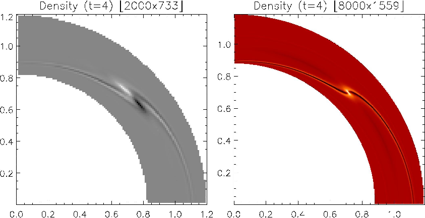
Vortices resolved on computational zones are persistent and, although affected by enhanced numerical viscosity and damping, still survived more than 20 revolutions. Otherwise, at least 24 grid points are necessary to correctly follow the nonlinear adjustment. In Fig 10 we show an example of such a situation, when numerical setup M (2000x733, 6 grid points over vortex) failed to describe the direct nonlinear adjustment of the initially imposed small-scale vortex, but displayed development of a dipolar or even tripolar vortex configurations. Direct nonlinear adjustment to the single long-lived structure is resolved only under considerably higher resolution (setup VH, 8000x1559, 24 grid points over the vortex) thus setting overall restriction on the resolution of our code.
Notwithstanding the fact that the purpose of the simulations is the study of small-scale vortices, global simulations are needed: vortices interact globally and change the density, temperature and potential vorticity in the whole ring at the radius where they are situated. Hence, to get a correct dynamical picture, we need true global simulations with a domain covering in azimuthal direction. Calculations on smaller domains in () have lead to drastically different results, since the two vortices at the same radius start to interact before the nonlinear adjustment occurs.
Another requirement on the numerical code is that it should be able to capture shocks, an important ingredient of the overall balance of the sustained structures in differentially rotating flows. In our case the PLUTO code employs solvers that accurately resolve the shock dynamics. This requirement does not play in favor of spectral codes for compressible simulations of the Keplerian disk dynamics.
7 Summary
Direct numerical simulations of the nonlinear dynamics of coherent vortices in 2D compressible protoplanetary disks with Keplerian differential rotation have been presented.
We have shown the possible existence of anticyclonic vortices with sizes exceeding the Keplerian disk height scales. We have followed the evolution of such vortices for 200 local revolutions, showing their persistence and stability.
We have found that the development of long-lived nonlinear anticyclonic vortex configurations occurs only when the amplitudes of the initially imposed vortex perturbations exceed some threshold value. We have distinguished two nonlinear threshold values, that define the fate of the initial vortex. At small amplitudes, the vortex behaves linearly and it decays due to the shearing deformation. When the amplitude exceeds the first threshold, the vortex stretching is followed by nonlinear instabilities, leading to the formation of multiple small-scale anticyclonic vortices. At amplitudes higher then the second threshold, direct transition from the initially unbalanced to the final equilibrium configuration occurs. We have interpreted the latter process as the nonlinear vortex adjustment and studied the parameters that can describe this process. We found that the vortex adjustment proceeds on two different time-scales. Shorter times are required for the settling the potential vorticity (3-6 revolutions) and longer time-scales are required for the adjustment of density. Density adjustment time-scales depend on the amount of viscosity present in the flow. Thus, we observe a transient double-core vortex, that evolves into a single core structure. The density core splitting of the vortex is due to the spiral shock induced compression. Cores tend to merge at later times and the process is promoted by the intrinsic numerical viscosity. At lower viscosity, double core vortices survive for longer times. The density at the center of the vortex slowly increases and the potential vorticity gradient steepens.
The structure of the developed long-lived vortex does not depends on the initial vortex configuration, provided it exceeds the second threshold amplitude and its size does not exceed a limiting value. In this sense we found a nonlinear attractor that is the final configuration of a wide range of initial vortical perturbations. We found a scaling law for the equilibrium vortex size. In particular we find that the ratio of the vortex size to the local disk scale height increases with the decrease of the sound speed. Therefore, at low sound speed the radial extent of equilibrium anticyclonic vortices can significantly exceed the disk thickness. In this case vortex dynamics is intrinsically 2D and should be well modelled by the present simulations. Note that the sound speed required is somewhat lower than the typical values expected for protoplanetary disks . In the expected range the radial extent would be of the order of the scale height, while the azimuthal extent will be five times larger, in this case, to have a conclusive answer, 3D calculations are needed.
Vortices generate density-spiral waves that rapidly develop into shocks. As a result, a long-lived nonlinearly balanced vortex is accompanied by two spiral compressible shock waves facing both radial directions. The shock strength is maximal in the vicinity of the vortex outer edge, where the shock is attached to the main vortex circulation and heats all the annular disk region containing the vortex. Higher resolution runs indicate that these shock waves are able to generate local potential vorticity and may support the vortex against viscous dissipation.
We analyzed cyclonic vortices at nonlinear amplitudes. It seems that the linear decay due to the shearing deformation is accelerated by nonlinear effects.
We performed a resolution study and found the necessity of a global high-resolution approach to numerical simulations of these processes. The fate of the vortex depends significantly on the dissipation properties of the code. So, in this sense the use of physical viscosity, as opposed to the intrinsic numerical viscosity present in our simulations, would improve understanding of the vortex behavior and damping.
Our study contributes to the scenario of planetary formation inside the core of the long-lived vortices. We found that protoplanetary disks with lower sound speed can sustain vortices with higher ratio of vortex size to disk thickness and create a more favorable conditions for dust trapping and mass accumulation. In this context, we have also found a steady increase of density inside the nonlinearly balanced vortex, partly, due to the existence of persistent, steady, spiral shock waves that we showed to be an intrinsic property of stationary vortices with sizes exceeding the half thickness of the disk.

Acknowledgements.
This work is supported by ISTC grant G-1217 and by italian MIUR. A.G.T. would like to acknowledge the hospitality of Osservatorio Asrtonomico di Torino. Numerical calculations have been partly performed in CINECA (Bologna, Italy) thanks to the support by INAF.References
- Adams & Watkins (1995) Adams, F. C. & Watkins, R. 1995, ApJ, 451, 314
- Barge & Sommeria (1995) Barge, P. & Sommeria, J. 1995, A&A, 295, L1
- Barranco & Marcus (2005) Barranco, J. A. & Marcus, P. S. 2005, ApJ, 623, 1157
- Bodo et al. (2005) Bodo, G., Chagelishvili, G., Murante, G., et al. 2005, A&A, 437, 9
- Bracco et al. (1999) Bracco, A., Chavanis, P. H., Provenzale, A., & Spiegel, E. A. 1999, Physics of Fluids, 11, 2280
- Chagelishvili et al. (1997) Chagelishvili, G. D., Tevzadze, A. G., Bodo, G., & Moiseev, S. S. 1997, Physical Review Letters, 79, 3178
- Chavanis (2000) Chavanis, P. H. 2000, A&A, 356, 1089
- Colella & Woodward (1984) Colella, P. & Woodward, P. R. 1984, Journal of Computational Physics, 54, 174
- Davis (2002) Davis, S. S. 2002, ApJ, 576, 450
- Davis et al. (2000) Davis, S. S., Sheehan, D. P., & Cuzzi, J. N. 2000, ApJ, 545, 494
- de la Fuente Marcos & Barge (2001) de la Fuente Marcos, C. & Barge, P. 2001, MNRAS, 323, 601
- Godon & Livio (1999a) Godon, P. & Livio, M. 1999a, ApJ, 521, 319
- Godon & Livio (1999b) Godon, P. & Livio, M. 1999b, ApJ, 523, 350
- Gottlieb & Shu (1998) Gottlieb, S. & Shu, C. W. 1998, Mathematics of Computation, 67, 73
- Johansen et al. (2004) Johansen, A., Andersen, A. C., & Brandenburg, A. 2004, A&A, 417, 361
- Johnson & Gammie (2005) Johnson, B. M. & Gammie, C. F. 2005, ApJ, 635, 149
- Klahr (2004) Klahr, H. H, 2004, ApJ, 606, 1070
- Klahr & Bodenheimer (2003) Klahr, H. H. and Bodenheimer, P., 2003, ApJ, 582, 869
- Klahr & Bodenheimer (2006) Klahr, H. H. and Bodenheimer, P., 2006, ApJ, 639, 432
- Koller et al. (2003) Koller, J., Li, H., & Lin, D. N. C. 2003, ApJ, 596, L91
- Lovelace et al. (1999) Lovelace, R. V. E., Li, H., Colgate, S. A., & Nelson, A. F. 1999, ApJ, 513, 805
- Lubow & Ogilvie (1998) Lubow, S. H. & Ogilvie, G. I. 1998, ApJ, 504, 983
- Masset (2000) Masset, F. 2000, A&AS, 141, 165
- Mignone et al. (2007) Mignone, A., Bodo, G., Massaglia, S., et al. 2007, ApJ, in press, ArXiv: astro-ph/0701854
- Papaloizou & Terquem (2006) Papaloizou, J. C. B. & Terquem, C. 2006, Reports of Progress in Physics, 69, 119
- Petersen et al. (2007) Petersen, M. P., Stewart, G. R. & Julien, K. 2007, ApJ, 658, 1252
- Schäfer et al. (2004) Schäfer, C., Speith, R., Günther, R., & Kley, W. 2004, Astronomische Nachrichten Supplement, 325, 85
- Shen et al. (2006) Shen, Y., Stone, J. M., & Gardiner, T. A. 2006, ApJ, 653, 513
- Tanigawa & Watanabe (2002) Tanigawa, T. & Watanabe, S.-i. 2002, ApJ, 580, 506
- Umurhan & Regev (2004) Umurhan, O. M. & Regev, O. 2004, A&A, 427, 855
- von Weiszacker (1944) von Weiszacker, C. F. 1944, Z. Astrophys., 22, 319