NSF-KITP-07-164
A prediction for bubbling geometries
Takuya Okuda
Kavli Institute for Theoretical Physics
University of California
Santa Barbara, CA 93106, USA
Abstract
We study the supersymmetric circular Wilson loops in Yang-Mills theory. Their vacuum expectation values are computed in the parameter region that admits smooth bubbling geometry duals. The results are a prediction for the supergravity action evaluated on the bubbling geometries for Wilson loops.
1 Introduction and summary
In a holographic correspondence, a quantum gravitational system is exactly equivalent to a non-gravitational theory on a lower dimensional space. In known examples [1, 2] the non-gravitational systems are gauge theories. Gauge invariant observables are mapped to non-normalizable deformations of the gravitational background.
Following progress in understanding the gravity duals of local operators in a gauge theory, the recent years have seen further extension of the dictionary to the realm of non-local gauge invariant operators. The picture that has emerged is strikingly universal for all local and non-local operators. Consider operators of the form , where the trace is evaluated in a representation of . We will often use the symbol to denote the associated Young diagram as well. For different representations , the operators are best described by different objects on the gravity side. The fundamental representation corresponds to a fundamental string. A high-rank symmetric representation corresponds to a D-brane, while an anti-symmetric representation is given by another type of D-brane. Finally, an operator with a large rectangular Young diagram is dual to a smooth bubbling geometry with a flux supported on a new cycle. A general Young diagram corresponds to a combination of these objects. This pattern, summarized in Figure 1, has been demonstrated for local operators [3, 4, 5, 6, 7] and Wilson loops [8, 9, 10, 11, 12, 13, 14, 15, 16, 17] in Yang-Mills, as well as for Wilson loops in Chern-Simons theory [2, 18, 19, 20]. Higher dimensional non-local operators [21, 22, 23, 16, 24, 25] in gauge theories have descriptions in terms of branes and bubbling geometries.

The identification of the operators and their dual bubbling geometries has been made on the basis of symmetries and charges. An interesting test of the identification, and AdS/CFT itself, would be to compare the expectation value of an operator with the on-shell supergravity action evaluated on the bubbling geometry. For most operators, however, the test is trivial. the expectation value vanishes for local operators, and does not depend on the coupling for the straight Wilson line. Even if the expectation value does not vanish, the computation in the gauge theory is usually done only in weak coupling. It is then hard to make comparison with the strong coupling computation performed on the gravity side.
In this paper we make a non-trivial prediction for the bubbling geometries dual to particular Wilson loops in Yang-Mills, by computing the vevs of the operators on the gauge theory side in the strong coupling regime. The operators are the circular supersymmetric Wilson loops defined as
| (1.1) |
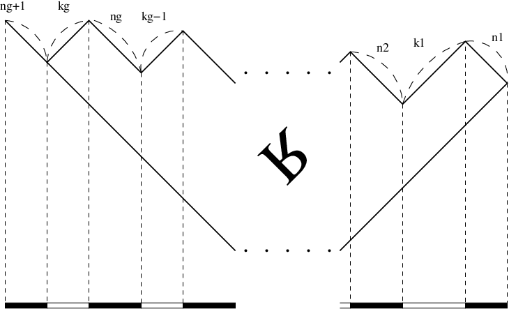
Here is the gauge field, () are the real scalars, is a parameter for a circle in Euclidean such that , and is a constant unit vector in . A smooth bubbling geometry is expected to be dual to a circular Wilson loop whose Young diagram has long edges. More precisely, if we parametrize the diagram as in Figure 2, for and for all have to be of order for the geometry to be smooth. The circular Wilson loop is very special in that such strong coupling computation from gauge theory is possible, due to the conjecture [26] that the Gaussian matrix model captures the circular Wilson loops to all orders in and the ’t Hooft coupling .
Relegating the computations to later sections, let us simply summarize the main result: in the limit with and kept finite, and for the large finite ’t Hooft coupling , the vev of the circular Wilson loop in the Yang-Mills with gauge group is given by
| (1.2) |
Here is the n-ality, i.e., the number of boxes in . We have also defined for and . An important check of the result is that it is invariant under complex conjugation of the representation, or in terms of the parameters, under
| (1.3) |
We expect that the Wilson loop vev is related to the on-shell supergravity action as
| (1.4) |
Note that in our regime. The quadratic dependence on of the exponent is what is expected from the supergravity action with , to be evaluated on the dual geometry.
This result is obtained by studying the Gaussian matrix model that captures the correlation functions of circular Wilson loops. In fact we turn the Gaussian matrix model with operator insertions into multi-matrix models whose partition functions are the Wilson loop vevs. We perform the saddle point analysis and propose the eigenvalue distributions. Based on this proposal, we are able to calculate the Wilson loop vevs with the result (1.2).
The circular Wilson loops in Euclidean can also be thought of as operators in the Yang-Mills defined on [26]. The loop is now the equator of , and the subgroup of the isometry group is preserved. The is part of the preserved subgroup of the conformal group . The operator (1.1) also preserves an subgroup of the R-symmetry group. Thus the bubbling geometry duals of the Wilson loops must solve the BPS equations of the type IIB supergravity with the ansatz. Note that we need to work with Euclidean signatures since the matrix model captures the circular loop in Euclidean only. The resulting geometries should be the Euclidean continuation of the solutions recently found in [17].
Given the result of the present paper, the challenge is to use the dual geometries to reproduce the prediction (1.2) by computing the on-shell supergravity action [27]. One would need to deal with such subtle issues as volume regularization, counter terms, and ambiguity of the action due to self-duality of the 5-form flux.11 1 The parallel problem of matching the Wilson loop vev and the closed string partition function has been solved for the Chern-Simons/conifold duality to all orders in genus expansion [18]. The matching of the Wilson loop vevs and the dual on-shell D-brane actions has also been demonstrated [10, 12, 13] for Yang-Mills.
Though the analysis of the matrix models for Yang-Mills is in principle sufficient, much confidence in the results and the proposed eigenvalue distributions comes from the study of surprisingly analogous matrix models that describe the Wilson loops in Chern-Simons theory [28, 29, 30]. For these matrix models, the resolvents and the spectral curves can be computed exactly in the limit , with and kept finite, without the assumption that the ’t Hooft coupling is large. The eigenvalue distributions turn out to be qualitatively the same for the Yang-Mills and Chern-Simons theory.
The paper is organized as follows. In section 2, we review the correspondence between the circular Wilson loops in Yang-Mills and the observables in the Gaussian matrix model. In section 3 we analyze the Wilson loop with a rectangular Young diagram. Section 4 deals with the Wilson loops in general representations that admit smooth dual bubbling geometries.
2 Gaussian matrix model for circular Wilson loops
It is believed [26, 31] that the correlation functions of circular loops in Yang-Mills are captured by the Gaussian matrix model. The precise correspondence states in particular that
| (2.5) |
The left-hand side is the normalized expectation value in the Yang-Mills with gauge group . The right-hand side is normalized by using the partition function which is the integral without the insertion of . is the standard hermitian matrix measure. In the absence of operator insertions, the eigenvalues are distributed according to the Wigner semi-circle law in the large limit. The eigenvalue density , normalized so that , is given by
| (2.6) |
We are also interested in the Yang-Mills theory, for which the conjecture in [26] states that
| (2.7) |
Note that on the right-hand side we need the traceless part
| (2.8) |
of the matrix so that . The relation
| (2.9) |
will be useful later.
Matrix integrals have been studied intensively in the past, partly motivated by non-critical string theory [32, 33] and relation to supersymmetric gauge theories [34, 35]. In these contexts one does not encounter operators of the form with the Young diagram that is large both in the row and column directions, and it appears that there is no study of them in the literature.22 2 I thank E. Martinec for a discussion on this point.
3 Rectangular Young diagram
In this section, we formulate 2-matrix models whose partition functions are the vev of the Wilson loop with a rectangular Young diagram shown in Figure 3. We will have two such matrix models. The first captures the geometric transition of D5-branes wrapping in . The second is similarly interpreted in terms of D3-branes wrapping . The techniques we introduce here are a generalization of the methods used in [13]. The pictures that emerge are similar to those of [12, 36].

3.1 Eigenvalues as D5-branes
We begin with the Yang-Mills with gauge group . Let be a unitary matrix and consider a sum over all the Young diagrams for which the summand is non-vanishing:
| (3.10) |
Here is the transpose of . This identity, expressed in terms of Schur polynomials as
| (3.11) |
is well-known [37]. The relation can be inverted:
| (3.12) |
Here is the Haar measure on the unitary group normalized so that . We now specialize to the rectangular Young diagram with rows and columns. We choose to be a unitary matrix. This choice has a considerable advantage. Let us recall the character formula [38]
| (3.13) |
where is the number of boxes in the -th row of . It implies that
| (3.14) |
for the rectangular diagram and for the matrix .33 3 This can also be understood as follows. A column of length gives the rank- anti-symmetric representation . The rectangular diagram is obtained by symmetrizing copies of . The representation for is one dimensional and the trace in is the determinant. Thus . By substituting (3.12) and (3.14) into (2.5), we conclude that
| (3.15) |
By diagonalizing the matrices as
| (3.16) |
and redefining , the vev can be written as
| (3.17) | |||||
The constant of proportionality is independent of and , is negligible in the precision we work with, and is thus dropped. Since the integrand is analytic, the contours of integration may be deformed. Each is integrated over a period .
The leading behavior of the Wilson loop vev in the large limit can be computed in the saddle point approximation. Note that all the terms in the exponent in (3.17) are of order . We thus expect a back-reaction of the -eigenvalue distributions to the -eigenvalues. This is in contrast to the case with a single row or column [13]. The saddle point equations are
| (3.18) | |||
| (3.19) |
One can get useful intuitions by interpreting these equations as force balance conditions. The first term in (3.18) is a restorative force on . The first term in (3.19) represents a constant force applied to each . These are the external forces acting on the system of eigenvalues. The other terms are mutual repulsive forces among ’s and ’s.
In the absence of -eigenvalues, the -eigenvalues obey Wigner’s semicircle law and spread over an interval of width . This motivates us to assume that the - and -eigenvalues spread over regions of length scale . Under this assumption that will be justified a posteriori, for large values of , we can approximate various expressions as follows:
We now propose an eigenvalue distribution that solves the saddle point equations. Suppose that the eigenvalues split into the first group on the right and the second one on the left. All the ’s are between them. We also assume that the two groups are far enough from each other so that can be ignored. After we apply (3.1) and (3.1), (3.18) becomes
| (3.26) | |||
| (3.27) |
Then the two groups individually obey Wigner’s semi-circle law. The first group is spread over an interval of width centered at . For the second group the interval is centered at the origin with width . (3.19) simplifies to
| (3.28) |
This equation is solved by ’s uniformly distributed along a line in the imaginary direction. The precise location of the line cannot be determined in this approximation. See Figure 4.

The parallel matrix model problem in the Chern-Simons case admits an exact solution for the finite ’t Hooft parameter [30]. It exhibits an essentially identical distribution of eigenvalues. This gives us confidence in our proposal of the distribution.
We now use the eigenvalue distribution to evaluate the Wilson loop vev. The exponent in (3.17) can be evaluated, with the help of (3.1) and (3.1), as
| (3.29) | |||||
The last term arises from completion of squares:
We thus conclude that
| (3.30) |
In the case, we need to work with defined in (2.8). Because of (2.9), the Wilson loop vev is given by
| (3.31) |
(3.29) is replaced by
| (3.32) |
The leading parts in comes from completion of squares:
We find that
| (3.33) | |||||
This is the special case of (1.2), and is invariant under or as it should be.
Recall that each column in represents a D5-brane. Since we have as many -eigenvalues as columns, we identify the eigenvalues with D5-branes. The back-reaction of the -eigenvalues to the existence of -eigenvalues then represents the back-reaction of the geometry to the branes, i.e., geometric transition. Without operator insertions, there is a single black region representing . The hole in the region, which was identified with D5-branes in [14], is created by the repulsion of and in the present formulation. This is the Wilson loop analog of giant graviton branes represented by a hole in the fermion droplet [7]. In the topological and non-critical string literature [39, 40], it is well-known that the insertion of a determinant operator similar to represents non-compact D-branes. In those cases the eigenvalues of are the moduli of branes. Here there is a difference: the eigenvalues are first integrated over and are fixed only by saddle point equations.
3.2 Eigenvalue bound states as D3-branes
If we make use of the identity [37, 38]
| (3.34) |
instead of (3.10), we have another expression for :
| (3.35) |
is the Haar measure on the unitary group. More precisely, the contours need to be deformed so that the eigenvalues of are larger than those of in magnitude. We choose to be an unitary matrix, so that
| (3.36) |
for the rectangular Young diagram . We find that the Wilson loop vev is given by another 2-matrix model
| (3.37) |
By diagonalizing the matrices, we get
| (3.38) | |||||
Let us now analyze this model in the limit with , and finite.
The saddle point equations are
| (3.39) |
and
| (3.40) |
Again these equations can be interpreted as force balance conditions for the eigenvalues. The difference from the previous subsection is that the interaction between and is attractive.
Let us study the eigenvalue distribution for finite but large . The -eigenvalues as a whole are pulled to the right by a force of magnitude . Unlike in the previous subsection, we cannot apply (3.1) and (3.1) to the terms involving and . If we did, would only be pulled to the right by , and the force balance would not be achieved. This suggests that each must be very close to .
Each -eigenvalue is pulled to the right by a force of magnitude . To balance this, we assume that the -eigenvalue and an -eigenvalue sit very close to each other. We also assume, as will be justified a posteriori, that this distance is much smaller than all other length scales in the problem. There are -eigenvalues and they are paired up with as many -eigenvalues (), forming bound states. The bound states are denoted by (-)a, . If we order the eigenvalues so that , is pushed to the right by .44 4 Strictly speaking, for such that (3.1) cannot be applied. The error from ignoring the effects, however, is cancelled by the error from ignoring the forces from with . It is also pushed to the left by , but these forces are cancelled by the pull of . Thus (3.40) in the approximation (3.1) becomes
| (3.41) |
The size of the -th bound state is thus .
Assuming that the group of bound states and the group of remaining -eigenvalues are far enough from each other, we can replace (3.39) by (3.26) and (3.27). Since the -eigenvalues are governed by the same equations as in the previous subsection, their distribution is the same. The distribution of the -eigenvalues is identical to the distribution of on the macroscopic scale. This then justifies the assumptions made in the argument. The computation of the Wilson loop vev is also identical.
Each row in the Young diagram represents a D3-brane [11, 15]. The rectangular diagram then corresponds to D3-branes. Since we have the same number of bound states, it is natural to identify each bound state with a D3-brane. This is the analog of an extra droplet in [7] where it was interpreted as dual giant graviton branes wrapping in .


4 General Young diagram
This section deals with a general Young diagram of the form shown in Figure 2, with edge lengths and all of order . We will obtain two multi-matrix models whose partition functions are the Wilson loop vev.
4.1 Eigenvalue bound states as D5-branes

Let us first see how to generalize the trick that led to 2-matrix models in the rectangle case. We begin with the expression
| (4.42) |
Here . Recall that . (3.13) in this case allows us to write
| (4.43) |
Here is obtained by removing the first rows from . See Figure 7. Similarly,
| (4.44) |
with in . To be more precise, to avoid singularities the integral is performed along the contours such that the eigenvalues of are larger than those of in magnitude. This time we have the relation
| (4.45) |
By removing the first rows from one obtains . We now repeat the procedure as many times as we can. This yields
| (4.46) | |||||
Here , and the integration contours are deformed so that the eigenvalues of have larger absolute values than those of .
We thus have
| (4.47) |
After redefining and diagonalizing the matrices as , , this becomes
| (4.48) | |||||
Our aim is to understand the behavior in the limit with finite, for large values of . The saddle point equations following from the action are
| (4.49) | |||
| (4.50) | |||
| (4.51) |
and
| (4.52) |
All the terms can be interpreted as forces on eigenvalues. Note that the interaction between and is repulsive, while the one between and is attractive. This suggests that some eigenvalues form bound states.

Let us work in the approximation. The following distribution of eigenvalues solves the saddle point equations. It involves types of bound states.55 5 Though it is convenient to talk about bound states, the size of a bound state is in fact of the same order as the distance to the neighboring bound state. The -th type of bound state, which we denote by (--…-), contains a single -eigenvalue for , as shown in Figure 8. The -eigenvalues split into groups . The (--…-)-bound states are distributed along a line in the imaginary direction, and separate from . See Figure 9. For interactions between two bound states or between a bound state and an -eigenvalue, we can apply (3.1) and (3.1). The (--…-)-bound state is pulled to the right by an external force of magnitude , and pushed back to the left by -eigenvalues from for . Bound states of different kinds do not interact with each other: forces cancel out among constituent eigenvalues. The saddle point equations are satisfied if the bound states are uniformly distributed along vertical lines. Calculation of relative positions of constituent eigenvalues in a bound state is straightforward. In the bound state (--…-), the distance between the - and -eigenvalues is for .

4.2 Eigenvalue bound states as D3-branes

Another matrix model can be obtained by starting with the formula
| (4.57) |
Here and is the Haar measure. We have defined . Note that
| (4.58) |
Here is obtained by removing the first rows from . See Figure 10. Similarly,
| (4.59) |
with essentially in . To avoid singularities the integral is performed along appropriate contours. We repeat the same procedure as many times as possible. This gives
| (4.60) | |||||
Here , and the integration contours are deformed so that the eigenvalues of have larger absolute values than .
We thus have
| (4.61) |
In terms of the eigenvalues, the Wilson loop is given by
| (4.62) | |||||
Let us study this model in the large limit with and fixed. The saddle point equations are
| (4.63) | |||
| (4.64) | |||
| (4.65) |
and
| (4.66) |
The forces between and as well as between and are attractive.

Our proposed distribution of the eigenvalues for large is as follows. There are types of bound states denoted by (--…-) for . Each bound state of the -th type has a single -eigenvalue as well as a single -eigenvalue for . The size of a bound state is of the order , and is much smaller than the distance between two neighboring bound states. The (--…-)-bound states are distributed according to the semi-circle law centered at . Using (3.1) and (3.1), one can confirm that the force balance among bound states is achieved. It is straightforward to calculate the distance between eigenvalues in a bound state. In the -th (--…-) bound state, the distance between the - and -eigenvalues turns out to be for . Here and . This configuration solves the saddle point equations. The distribution of the -eigenvalues is identical to the one in the previous subsection, and leads to the same results for the Wilson loop vev.

Acknowledgments
I thank Jaume Gomis and Kentaroh Yoshida for helpful conversations. I am especially grateful to Sean Hartnoll for many useful discussions, and Nick Halmagyi for collaboration on a related project [30]. I also acknowledge the hospitality of the Simons Workshop at Stony Brook, where this work was completed. My research is supported in part by the NSF grants PHY-05-51164 and PHY-04-56556.
References
- [1] J. M. Maldacena, “The large N limit of superconformal field theories and supergravity,” Adv. Theor. Math. Phys. 2 (1998) 231–252, hep-th/9711200.
- [2] R. Gopakumar and C. Vafa, “On the gauge theory/geometry correspondence,” Adv. Theor. Math. Phys. 3 (1999) 1415–1443, hep-th/9811131.
- [3] J. McGreevy, L. Susskind, and N. Toumbas, “Invasion of the giant gravitons from anti-de Sitter space,” JHEP 06 (2000) 008, hep-th/0003075.
- [4] A. Hashimoto, S. Hirano, and N. Itzhaki, “Large branes in AdS and their field theory dual,” JHEP 08 (2000) 051, hep-th/0008016.
- [5] V. Balasubramanian, M. Berkooz, A. Naqvi, and M. J. Strassler, “Giant gravitons in conformal field theory,” JHEP 04 (2002) 034, hep-th/0107119.
- [6] S. Corley, A. Jevicki, and S. Ramgoolam, “Exact correlators of giant gravitons from dual N = 4 SYM theory,” Adv. Theor. Math. Phys. 5 (2002) 809–839, hep-th/0111222.
- [7] H. Lin, O. Lunin, and J. M. Maldacena, “Bubbling AdS space and 1/2 BPS geometries,” JHEP 10 (2004) 025, hep-th/0409174.
- [8] J. M. Maldacena, “Wilson loops in large N field theories,” Phys. Rev. Lett. 80 (1998) 4859–4862, hep-th/9803002.
- [9] S.-J. Rey and J.-T. Yee, “Macroscopic strings as heavy quarks in large N gauge theory and anti-de Sitter supergravity,” Eur. Phys. J. C22 (2001) 379–394, hep-th/9803001.
- [10] N. Drukker and B. Fiol, “All-genus calculation of Wilson loops using D-branes,” JHEP 02 (2005) 010, hep-th/0501109.
- [11] J. Gomis and F. Passerini, “Holographic Wilson loops,” JHEP 08 (2006) 074, hep-th/0604007.
- [12] S. Yamaguchi, “Wilson loops of anti-symmetric representation and D5- branes,” JHEP 05 (2006) 037, hep-th/0603208.
- [13] S. A. Hartnoll and S. P. Kumar, “Higher rank Wilson loops from a matrix model,” JHEP 08 (2006) 026, hep-th/0605027.
- [14] S. Yamaguchi, “Bubbling geometries for half BPS Wilson lines,” Int. J. Mod. Phys. A22 (2007) 1353–1374, hep-th/0601089.
- [15] J. Gomis and F. Passerini, “Wilson loops as D3-branes,” JHEP 01 (2007) 097, hep-th/0612022.
- [16] O. Lunin, “On gravitational description of Wilson lines,” JHEP 06 (2006) 026, hep-th/0604133.
- [17] E. D’Hoker, J. Estes, and M. Gutperle, “Gravity duals of half-BPS Wilson loops,” arXiv:0705.1004 [hep-th].
- [18] J. Gomis and T. Okuda, “Wilson loops, geometric transitions and bubbling Calabi- Yau’s,” JHEP 02 (2007) 083, hep-th/0612190.
- [19] J. Gomis and T. Okuda, “D-branes as a Bubbling Calabi-Yau,” JHEP 07 (2007) 005, arXiv:0704.3080 [hep-th].
- [20] T. Okuda, “BIons in topological string theory,” arXiv:0705.0722 [hep-th].
- [21] S. Gukov and E. Witten, “Gauge theory, ramification, and the geometric langlands program,” hep-th/0612073.
- [22] J. Gomis and S. Matsuura, “Bubbling surface operators and S-duality,” JHEP 06 (2007) 025, arXiv:0704.1657 [hep-th].
- [23] A. Karch and L. Randall, “Open and closed string interpretation of SUSY CFT’s on branes with boundaries,” JHEP 06 (2001) 063, hep-th/0105132.
- [24] J. Gomis and C. Romelsberger, “Bubbling defect CFT’s,” JHEP 08 (2006) 050, hep-th/0604155.
- [25] O. Lunin, “1/2-BPS states in M theory and defects in the dual CFTs,” arXiv:0704.3442 [hep-th].
- [26] N. Drukker and D. J. Gross, “An exact prediction of N = 4 SUSYM theory for string theory,” J. Math. Phys. 42 (2001) 2896–2914, hep-th/0010274.
- [27] T. Okuda and D. Trancanelli. Work in progress.
- [28] M. Marino, “Chern-Simons theory, matrix integrals, and perturbative three-manifold invariants,” Commun. Math. Phys. 253 (2004) 25–49, hep-th/0207096.
- [29] M. Aganagic, A. Klemm, M. Marino, and C. Vafa, “Matrix model as a mirror of Chern-Simons theory,” JHEP 02 (2004) 010, hep-th/0211098.
- [30] N. Halmagyi and T. Okuda, “Bubbling Calabi-Yau’s from matrix models.” To appear.
- [31] J. K. Erickson, G. W. Semenoff, and K. Zarembo, “Wilson loops in N = 4 supersymmetric Yang-Mills theory,” Nucl. Phys. B582 (2000) 155–175, hep-th/0003055.
- [32] P. H. Ginsparg and G. W. Moore, “Lectures on 2-D gravity and 2-D string theory,” hep-th/9304011.
- [33] P. Di Francesco, P. H. Ginsparg, and J. Zinn-Justin, “2-D Gravity and random matrices,” Phys. Rept. 254 (1995) 1–133, hep-th/9306153.
- [34] R. Dijkgraaf and C. Vafa, “Matrix models, topological strings, and supersymmetric gauge theories,” Nucl. Phys. B644 (2002) 3–20, hep-th/0206255.
- [35] R. Dijkgraaf and C. Vafa, “A perturbative window into non-perturbative physics,” hep-th/0208048.
- [36] S. Yamaguchi, “Semi-classical open string corrections and symmetric Wilson loops,” JHEP 06 (2007) 073, hep-th/0701052.
- [37] I. Macdonald, Symmetric functions and Hall polynomials. Oxford, second ed., 1995.
- [38] J. Fulton and W. Harris, Representation Theory: A First Course. Graduate Texts in Mathematics. Springer-Verlag, 1999.
- [39] M. Aganagic, R. Dijkgraaf, A. Klemm, M. Marino, and C. Vafa, “Topological strings and integrable hierarchies,” Commun. Math. Phys. 261 (2006) 451–516, hep-th/0312085.
- [40] J. M. Maldacena, G. W. Moore, N. Seiberg, and D. Shih, “Exact vs. semiclassical target space of the minimal string,” JHEP 10 (2004) 020, hep-th/0408039.