Ignition latitude and the shape of Type I X-ray bursts
Abstract
The shape of the lightcurve during the rising phase of Type I X-ray bursts is determined by many factors including the ignition latitude, the accretion rate, and the rotation rate of the star. We develop a phenomenological model of the burst rise process and show that simple measures of the burst morphology can be robust diagnostics of ignition latitude and burning regime. We apply our results to the large sample of bursts from the Low Mass X-ray Binary 4U 1636-536, and find evidence for off-equatorial ignition for many of the bursts. We argue that such behaviour may be associated with the transition from hydrogen to helium ignition at accretion rates a few percent of Eddington. We show that this model can also explain variations in the detectability of burst oscillations, and discuss the implications for other burst sources.
Keywords:
binaries: general – stars: individual: 4U 1636-536 – stars: neutron– stars: rotation – X-rays: bursts – X-rays: stars1 Introduction
Neutron stars in Low Mass X-ray Binaries (LMXBs) accrete matter from their low mass companions via Roche lobe overflow. Nearly half of these systems show Type I X-ray bursts, thermonuclear flashes caused by rapid unstable burning of the accumulating hydrogen or helium after it settles and is compressed on the neutron star surface. A typical X-ray burst light curve has a rapid rise (less than 10 s), followed by a longer decaying tail persisting for seconds to minutes as the star’s surface cools.
The basic properties of Type I X-ray bursts can be understood in terms of the stability of hydrogen and helium burning at different accretion rates (Fujimoto, Hanawa & Miyaji 1981; Fushiki & Lamb 1987; Bildsten 1998; Bildsten 2000; Narayan & Heyl 2003; Woosley et al. 2004; Cooper & Narayan 2006; Peng, Brown & Truran 2007). The boundaries between the different burning regimes depend on the local accretion rate (accretion rate per unit area). Below a critical accretion rate % of the Eddington rate , bursts are triggered by unstable hydrogen burning. Above this level, hydrogen burns stably via the hot CNO cycle, and bursts are triggered by unstable helium burning once a critical column depth is reached. For but below a second critical rate , expected to be a few percent of , the hydrogen at ignition depth should burn before helium ignition, leading to a pure helium flash. At higher accretion rates, , hydrogen does not burn completely before the burst is triggered, leading to various classes of mixed H/He bursts. Bursting activity will cease when the accretion rate is sufficiently high, , that helium burning is also stable. The precise levels of the critical accretion rates , , are not known precisely and will vary depending on factors such as the metallicity of the accreted material and the heat flux from the deep crust and core (Ayasli & Joss 1982; Fushiki & Lamb 1987; Brown, Bildsten & Rutledge 1998; Narayan & Heyl 2003).
There is now observational evidence for bursts in all three classes. The global accretion rate can be inferred from the X-ray luminosity, and this should (under the assumption that accretion is spherically symmetric) predict and hence the burning regime. Furthermore, within a given burning regime, burst rate should rise with accretion rate. For a large number of sources, however, these expectations are not borne out. Transition accretion rates can differ from the predicted values by up to an order of magnitude, and for many sources burst rate actually falls as increases (Cornelisse et al. 2003; Galloway et al. 2007). Why this should be the case is not yet clear but it may involve either additional stable burning processes (Bildsten 1995) or non-spherical accretion and slow fuel spread (so that local accretion rate differs from that inferred from ) (Bildsten 2000). Alternatively it may well be that X-ray luminosity is not a good predictor of accretion rate (Hasinger & van der Klis 1989). For a more in-depth discussion of these issues and other burst properties we refer the reader to the recent articles by Strohmayer & Bildsten 2006 and Galloway et al. 2007.
In this paper we concentrate on one particular aspect of burst physics - the properties of the burst rise. The shape and time scale of the rising portion of the X-ray light curve is controlled by several factors: the point at which the burning layer ignites, the emission profile of any burning point after ignition (set by the nuclear heating and cooling time scales); and the speed at which the burning front propagates across the stellar surface. Ignition is likely to occur at a point and spread, rather than occurring across the whole star simultaneously, because of the discrepancy between the very short burning time scales and the much longer accretion time scale (Shara 1982). Asymmetric initialization is also thought necessary to explain the detection during the rise of burst oscillations, variations in brightness on the surface of the neutron star that are modulated by the rapid stellar spin (Strohmayer & Bildsten 2006).
On a realistic neutron star, ignition location is unlikely to be random due to the various factors that break spherical symmetry. Accretion flow may not be spherically symmetric - it may occur through an equatorial boundary layer (Inogamov & Sunyaev 1999) or by channeling onto the magnetic poles (in which case the star may manifest as an X-ray pulsar). Whether either of these issues can affect local ignition conditions or lead to preferred ignition locations is not clear, since estimates suggest that fuel should spread rapidly across the stellar surface between bursts. Another factor that will certainly have an impact is stellar rotation. Most of the neutron stars that show Type I X-ray bursts are thought to be rapidly rotating, which reduces the effective gravity at the equator. Centrifugal effects, coupled with the deformation of the neutron star due to the rapid rotation, combine to reduce the effective gravity at the equator as compared to the poles. This results in a local accretion rate that is higher at the equator (Spitkovsky, Levin & Ushomirsky 2002). The column depth required for ignition is achieved more rapidly, and ignition should occur preferentially at this latitude. In fact there are accretion rates where off-equator ignition is still expected. Cooper & Narayan 2007a considered the situation at high accretion rates where helium burning is on the verge of stability. There will be a range of accretion rates (the more rapid the rotation, the larger this range) where at the equator but not at other latitudes. Although not discussed by Cooper & Narayan 2007a, a similar region of off-equator ignition is to be expected at (the transition to stable hydrogen burning).
Once ignition has occurred, the nuclear burning processes determine the emission from a given point. The burning layer will expand during a convective phase, and there is a delay before radiative processes take over and the light curve starts to rise. Light curves from a single point (ignoring spreading effects) have been generated by a number of authors (Taam 1980; Ayasli & Joss 1982; Fushiki et al. 1992; Taam et al. 1993; Woosley et al. 2004; Weinberg, Bildsten & Schatz 2006). The shape, time scales and strength of the single point light curve can vary substantially depending on factors such as the burning regime and the composition of the accreted material. There are as yet no simple analytic models for this process that take into account all of the relevant parameters.
At the accretion rates of relevance to most burst sources, the burning front is expected to propagate by deflagration (Fryxell & Woosley 1982b; Hanawa & Fujimoto 1984; Bildsten 1995) rather than by detonation (Fryxell & Woosley 1982a; Zingale et al. 2001). In the simplest picture, spreading speed is set by the rate at which heat is transported across the burning front (by convective processes). Spitkovsky, Levin & Ushomirsky 2002 have since shown that rapid rotation will also play a significant role: interaction between the uplift (vertical expansion) of burning material and a strong Coriolis force can act to slow spreading. The degree of asymmetry in the spread of the burning front is also relevant to the detectability of burst oscillations in the rise, if they are caused by a growing hot spot.
In this paper we attempt the first systematic examination of how these various factors interact to affect the shape and time scale of the rising portion of the light curve. Previous studies in this area have focused on small samples of bursts such as the rare multi peaked bursts (Bhattacharyya & Strohmayer 2006a; Bhattacharyya & Strohmayer 2006b), or bursts from the accreting millisecond pulsars (Bhattacharyya & Strohmayer 2006c). In this study we adopt a much broader remit, motivated by the wide variety of shapes exhibited by the bursts of the LMXB 4U 1636-536. This particular source is an excellent candidate for this type of study: there are over 120 bursts from this source in the Rossi X-ray Timing Explorer (RXTE) archive, and it lies in a binary with relatively well-constrained properties. By comparing the burst properties with the results of parameterized simulations, we show that simple measures of the burst shape can be profound diagnostics of ignition latitude and burning regime.
The paper is structured as follows. In Section 2 we define simple measures of burst morphology and classify the bursts of 4U 1636-536 accordingly. Section 3 gives details of the parameterized simulations that we carried out to generate model light curves, and looks at the effects on shape using the same simple measures. In Section 4 we compare the results of our simulations with the data, and consider the implications in terms of ignition point and burning regime. We present a model that can explain our results (subject to the assumptions inherent in our simulations), and extend our analysis to other sources to test its feasibility. We conclude in Section 5.
2 Observational data analysis
The bursting LMXB 4U 1636-536 is a persistent atoll source at a distance of kpc (Galloway et al. 2006) in a 3.8 hour binary orbit with a low mass blue star, V801 Ara. The binary inclination is in the range (Casares et al. 2006). The bursts have been studied extensively with both EXOSAT (Lewin, van Paradijs & Taam 1993) and RXTE (Galloway et al. 2007). Burst oscillations at 581 Hz are seen in both normal bursts and superbursts, the latter being longer bursts triggered by unstable carbon burning (Strohmayer et al. 1998; Strohmayer & Markwardt 2002). We include in our study all of the bursts covered by the RXTE burst catalogue (Galloway et al. 2007). The catalogue includes over 1000 bursts observed by the RXTE Proportional Counter Array (PCA) from December 30th 1995 to October 29th 2005, 123 of which originate from 4U 1636-536.
In order to study the shape and time scales of the bursts’ rises we started by constructing light curves from the PCA data, using Standard 1 data (0.125 s resolution) and using all available energy channels. For most of the bursts this results in a smooth and monotonically increasing light curve. For a small group of bursts with peak fluxes below ergs cm-2 s-1 (bursts 11, 67, 71, 76, 78, 87, 88, 91, 118 and 122 for this source, using the numbering system of Galloway et al. 2007), the light curve is not smooth, so we exclude these bursts from our analysis. Burst 117 is also excluded because the rise is truncated. We also exclude for the moment bursts that are either kinked or multi-peaked when plotted on a coarser (0.5s) time resolution: that is to say bursts where the gradient of the lightcurve drops to zero or below during the rise. This group includes the strongly multi-peaked bursts (40, 48, 56 and 111) identified as such by Galloway et al. 2007 as well as a group that are either kinked or weakly multi-peaked (bursts 5, 18, 90, 110 and 113), see Figure 1. We will discuss these bursts in more detail in Section 4.

In analyzing the light curves of the remaining 103 bursts we considered several different ways of quantifying the shape. The measure that we found to be most powerful, which we call convexity (), measures the degree to which the light curve is concave or convex. The physical significance of this parameter will become clear in Section 3, where we find that it can be used to diagnose the latitude at which the burst ignites. Convexity is calculated as follows. We define the burst rise to be the interval where the count rate rises from 10 to 90 percent of the maximum count rate (corrected for the pre-burst persistent emission). We define rise time as the duration of that interval. In order to compare the shape of bursts of different durations and peak count rates we then normalize both quantities so that they rise from 0 to 10 in dimensionless units. This process is illustrated in Figures 2 and 3. Taking as the re-normalized count rate in each bin, and as the identity function (shown as a diagonal line in Figure 3), we define convexity as
| (1) |
where N is the number of re-normalized time bins and is the re-normalized time bin size. Convexity is effectively the integrated area of the curve above or below the diagonal line - areas above the line being positive and areas below negative. For highly convex bursts, where most points lie above the diagonal, is positive, and for highly concave bursts it is negative. Our choice of re-normalization means that lies in the range -50 to 50.


Figure 4 plots the peak flux of the bursts against convexity. At high peak fluxes almost all of the bursts have , whereas at low peak fluxes we find equal numbers of bursts with both positive and negative convexities. For convenience in later discussions, we assign the bursts to three broad groups, as indicated in the Figure. Bursts with ergs cm-2 s-1 are assigned to Group 1 () or Group 2 (), while the bright photospheric radius expansion (PRE) bursts with ergs cm-2 s-1 form Group 3. There are no PRE bursts in Group 1, and only one in Group 211 1 Burst 16, identified by Galloway et al. 2006 as a PRE burst with an anomalously low peak flux, due most likely to the presence of hydrogen..
Figures 5 and 6 show the relationship between accretion rate and burst rise time22 2 Note that we use a different definition of rise time to Galloway et al. 2007. These authors define rise time as the time taken for the count rate to rise from 25% to 90% of the peak rate. for the bursts. Galloway et al. 2007 give two parameters that can be used to estimate the accretion rate at the time of the burst. The first, the normalized persistent flux , is the ratio of the persistent X-ray flux to the Eddington flux. This is thought to be a reasonable estimate of the global accretion rate as a fraction of the Eddington rate . The second measure, , measures position in a colour-colour diagram: is thought to increase as accretion rate rises. Both measures show the same trend. The bursts in Groups 1 and 2 cluster at low accretion rates (a few percent of Eddington) and have longer rise times than those in Group 3. The Group 3 bursts have short rise times and dominate at higher accretion rates.


Table 1 summarizes the mean properties of the three groups of bursts. In addition to the parameters previously defined, we include burst fluence (the integrated flux during the whole burst) and the burst time scale (the ratio of burst fluence to peak flux), using data from Galloway et al. 2007. Group 3 bursts have higher fluences and shorter time scales, whereas properties for Groups 1 and 2 are similar. We also indicate the percentage of bursts in each group for which Galloway et al. 2007 state that oscillations are detected during the burst rise phase. Oscillations are far more prevalent in Group 3 than in Groups 1 and 2, as previously noted for this source by Muno et al. 2001.
| Property | Group 1 | Group 2 | Group 3 |
|---|---|---|---|
| Number of bursts in group | 31 | 30 | 42 |
| (s) | 3.3 1.0 | 2.8 1.6 | 1.2 0.3 |
| (s) | 10.8 4.9 | 13.7 6.6 | 7.7 2.2 |
| (10-6 ergs cm-2) | 0.24 0.02 | 0.33 0.03 | 0.48 0.02 |
| 0.033 0.003 | 0.033 0.003 | 0.052 0.003 | |
| 1.91 0.06 | 1.69 0.08 | 2.13 0.03 | |
| (10-9 ergs cm-2 s-1) | 22.7 1.8 | 25.5 1.9 | 62.7 0.8 |
| % bursts with oscillations in rise | 7% | 23% | 36% |
3 Simulations
To understand what might cause the variations in shape and time scale seen in the observational data, we developed a simple phenomenological model of the burst rise process and ran parameterized simulations to generate light curves. Our model consists of three main elements: a time-dependent temperature profile used to describe the emission from each point on the surface after ignition; a velocity model that describes the propagation of the burning front across the neutron star surface; and a light curve generation routine that models the propagation of photons from the neutron star surface towards a distant observer.
To generate light curves we use the Oblate Schwarzschild (OS) approximation of Morsink et al. 2007 to model relativistic light-bending, Doppler shifts and gravitational redshift. The OS model, which takes into account rotation-induced oblateness, is more appropriate for very rapidly rotating neutron stars than the more usual Schwarzschild + Doppler approximation (Poutanen & Gierliński 2003). Assuming that burst oscillation frequency is a good measure of stellar spin33 3 For the two accreting millisecond pulsars that also show burst oscillations, the burst oscillation frequency is at or very close to the known spin frequency (Chakrabarty et al. 2003; Strohmayer et al. 2003). The situation for the non-pulsing LMXBs is less clear (there are some differences in burst oscillation properties compared to the pulsars, see Watts & Strohmayer 2006). However, in all of the suggested models (Section 1) burst oscillation frequency lies within a few Hz of the spin frequency., 4U 1636-536 rotates at Hz. The associated rotational deformation is a few percent, depending on the assumed mass and nuclear equation of state, leading to a small but noticeable influence on the light curve (Morsink et al. 2007). We neglect both special relativistic time delay and the additional time delay experienced by initially inwardly propagating photons, since these delays are much smaller ( s, Poutanen & Beloborodov 2006) than the time bins we consider ( s). We specify stellar mass and equatorial radius and then compute the deformed spherical surface using the OS model.
To start the burst we specify an initial small burning area and then track the propagation of the burning front across the star. The stellar surface is divided into a grid of patches with area 0.1 km2, and we consider a patch to be ignited as soon as the burning front reaches the centre point of the patch. Once a patch has started burning, we need to specify how its emission varies with time. As discussed in Section 1, there are various numerically-generated single point emission models, but no simple analytic models. In this study we follow Bhattacharyya & Strohmayer 2006a; Bhattacharyya & Strohmayer 2006b and assume that the temperature of the burning front follows the following profile after ignition:
| (2) | |||||
where is the time at which the temperature reaches its maximum . The time scale sets the time scale at which the temperature increases, while sets the time scale on which it decays. Unburnt patches are assumed to have a temperature until ignition. The parameters in this model depend primarily on the composition of the burning material, which will vary with on accretion rate (see Section 1). Bursts which are helium-rich, for example, would be expected to have shorter timescales than those which contain a higher fraction of hydrogen. Our parameter space must therefore be wide enough to take into account the expected level of variation. One follow-on question is whether this exponential temperature model remains valid across all burning regimes. It has been used successfully in detailed spectral modelling of bursts at different accretion rates by Bhattacharyya & Strohmayer 2006a; Bhattacharyya & Strohmayer 2006b, but ultimately one would like to see this confirmed by detailed nuclear physics calculations.
We then assume black body emission at the specified temperature from each patch. In Figure 7 we show the typical single patch light curve. The rise portion is similar in shape to the bursts shown in Woosley et al. 2004. The decay portion does differ from that seen in some of the cases studied by Woosley et al. 2004, but because we are focusing on the rise we never reach the points late in the decay phase where the difference would become relevant. This relatively simple analytic formulation is therefore a reasonable approximation to a more realistic calculation, for the short rising phase that we are studying. To this we can then apply various different beaming functions.
In adopting this emission model we have made two assumptions. We have assumed that each point on the star will have the same emission profile. This may not be the case, since emission could vary (as a result, say, of inhomogeneities in fuel deposition or composition). We have also neglected any delay between ignition and emission. If a convective zone develops there will be a delay as the zone grows before radiative processes become a more efficient form of transport, and radiation starts to escape from the photosphere (Weinberg, Bildsten & Schatz 2006). If this delay is position-independent then there will be no effect on the overall shape of the lightcurve; there could however be some position-dependence here that would contribute to variations in emission profile across the star.

In modeling the spreading of the burning front, we use the expression for burning front speed, , developed by Spitkovsky, Levin & Ushomirsky 2002. This speed depends on various nuclear burning parameters as well as the (poorly known) strength of frictional coupling between the top and bottom of the burning ocean. In general the velocity is latitude dependent (faster at the equator), because of the role of the Coriolis force. Spitkovsky, Levin & Ushomirsky 2002 show that the burning front speed varies as
| (3) |
In this expression, is the acceleration due to gravity at the surface, is the scale height of the hot burnt material, and is the Coriolis parameter, being the angular frequency the star and the latitude. The parameter is the time scale for frictional coupling between the top and bottom layers of the burning ocean. The parameter is the nuclear time scale of the thermonuclear burning (set by the composition of the burning material), and is a constant of order unity. In the case of weak frictional coupling ()44 4 Note that this approximation breaks down in a very small region near the equator, where . In this case we have to use the full expression for velocity.
| (4) |
where the velocity at the pole, . If frictional effects are stronger (), behaviour depends on how compares to . Maximum flame speed is reached when . In this case
| (5) |
with . In the high frictional coupling limit () the latitude dependence disappears, and
| (6) |
The shape of the light curve depends on a whole host of parameters: however some have a larger effect than others. We start by presenting results for a baseline scenario, where some of the parameters are fixed. Later in this section we will show that varying these additional parameters has only a limited effect on our findings. In the baseline scenario we assume a neutron star mass and an equatorial radius km. We set the spin rate of the neutron star to 580 Hz, and assume a binary inclination , in the middle of the range inferred for 4U 1636-536 by Casares et al. 2006. In the spreading speed model we assume that frictional coupling is weak (equation 4), so that flame speed is inversely proportional to . We start our simulations by setting an initial burning area with radius 1 km, similar to the expected width of the flame front (Spitkovsky, Levin & Ushomirsky 2002). In the temperature model (equation 2) we fix the following parameters: keV, keV, and s (as used by Bhattacharyya & Strohmayer 2006a). We also assume beaming , where is the angle from the normal to the surface.
The parameters that we vary are the ignition latitude , the polar velocity and the temperature rise time scale . We vary ignition latitude in steps from (north pole) to (south pole). The parameters and both depend on the composition of the burning material, which will vary with accretion rate as the fraction of hydrogen changes. We choose ranges for these parameters wide enough to encompass the level of variation that might be expected as we move from pure helium bursts to hydrogen-rich bursts (Woosley et al. 2004; Weinberg, Bildsten & Schatz 2006). We consider cm/s (for velocities outside this range our simulations give rise times are either much shorter or much longer than those observed). In the temperature profile we consider s, a range wide enough to cover the values generated in the single point light curve models of, for example, Weinberg, Bildsten & Schatz 2006.

Figure 8 shows the results from our simulations. It is clear that ignition latitude has a dramatic effect on both convexity and rise times. We find the following key result: bursts ignited on the equator always have , for the full range of and considered. Convexity decreases as ignition latitude moves towards the poles, and can eventually become negative at high enough latitudes; negative convexity being much more easily achieved when ignition starts in the northern hemisphere than in the southern. Rise times do vary slightly with ignition latitude but depend more strongly on spreading speed and the temperature rise timescale. The differences between northern and southern hemisphere ignition are due to the fact that we are observing the star from a northern hemisphere vantage point (). For bursts ignited at the south pole we do not observe the initial slow, concave, part of the rise that is visible to us if the burst ignites at the north pole. A south pole ignited burst therefore appears to have a higher convexity, purely by virtue of our viewing angle.
Let us now consider whether our results are robust when we vary the parameters that were held constant in our previous simulations: neutron star mass and radius, inclination angle, and the size of the initial burning area. We also vary the remaining temperature parameters, which are functions of composition and hence accretion rate. To do this we took a representative sample of bursts (Table 2), varied the other parameters, and compared the results to the baseline scenario with the same ignition latitude, and .
| Burst ID | (∘) | ( cm/s) | (s) |
| 1 | 0 | 2 | 0.1 |
| 2 | 0 | 2 | 0.5 |
| 3 | 0 | 4 | 0.1 |
| 4 | 0 | 4 | 0.5 |
| 5 | 90 | 2 | 0.1 |
| 6 | 90 | 2 | 0.5 |
| 7 | 90 | 8 | 0.1 |
| 8 | 90 | 8 | 0.5 |
| 9 | 180 | 2 | 0.1 |
| 10 | 180 | 2 | 0.5 |
| 11 | 180 | 4 | 0.1 |
| 12 | 180 | 4 | 0.5 |
We considered neutron star masses in the range to and equatorial radii 10 to 14 km, in line with reasonable estimates for a range of equations of state (Lattimer & Prakash 2007). We varied inclination from to (a range much larger than that inferred for 4U 1636-536, but which will allow us to extend our results to other sources in Section 4). The radius of the initial burning region was varied from 200 m to 1 km. We took in the range 4-15 s, and tested the effect of increasing both and by a factor of 5. We also included the effect of the RXTE spacecraft response on our simulated bolometric light curves. To do this we generated typical PCA response functions using some of the observed bursts analyzed in Section 2. We then used XSPEC to fold our simulated light curves through the response functions, and re-computed convexity and rise times for the folded light curves.
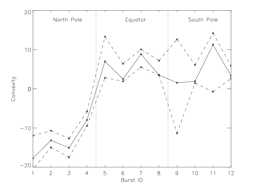


Figures 9 and 10 show the deviations in (respectively) convexity, and burst rise time, as compared to the standard scenario, for inclinations in the range (the range appropriate for 4U 1636-536). The results of our previous analysis are clearly robust. In Figure 11 we show results for a much wider range of inclinations. The range of variation is much wider, but again our main conclusions stand: negative convexity requires off-equatorial ignition.
We also checked the effects of several other parameters that are not shown in the Figures. One thing that we tested was the effect of changing the beaming factor. We first tried removing the beaming factor: this had very little effect on bursts ignited in the northern hemisphere or at the equator. Burst ignited in the southern hemisphere, however, were more prone to having negative convexities. We also tried the more physically motivated grey atmosphere model (Miller & Lamb 1998). In this model, the temperature of each patch
| (7) |
where is the effective temperature of the emitting layer and is the angle from the normal. The effect on convexity was extremely small compared to the baseline scenario (as might be expected, since both have the same dependence).
We also varied the latitude-dependence of spreading speed. In the baseline scenario we assumed that we were in the low frictional coupling regime, where latitude-dependence is strongest (). By the intermediate friction regime, , while in the highest friction regime the dependence on latitude vanishes. We therefore considered two additional models, and . Interestingly both of these models failed to reproduce the observed convexities. The constant velocity case produced no negative convexity bursts at all. The intermediate friction case did generate some bursts with but the values were not sufficiently negative to match the observations.
4 Discussion
4.1 Ignition latitude and burning regime
We start by summarizing the most important results from the preceding sections. In our analysis of the bursts of 4U 1636-536, we identified three populations: one group with higher peak fluxes and two groups with lower peak fluxes. The high peak flux group dominate at higher accretion rates and have short rise times. All but two of the members of this group have positive convexity. The lower peak flux bursts divide into two groups of similar size: one with positive convexity and one with negative convexity. Rise times in this group are longer than for the high peak flux group, suggesting a different burning regime.
In our simulations, both composition of the burning material (hydrogen fraction) and ignition latitude have a strong influence on convexity (Figure 8). However only bursts that ignite near the poles have negative convexities: bursts ignited on or near the equator always have positive convexity. In addition, bursts ignited near the north pole always have lower convexity than those ignited near the south pole. We can therefore draw the following conclusion55 5 Subject, of course, to the assumptions in our modeling. Negative convexity bursts could, for example, be generated by equatorial ignition if the single point lightcurves were concave rather than convex (see Figure 7). Although we are not aware of any physical motivation for such an assumption, we ran several simulations with concave single point lightcurves to study the possibility. In these simulations, however, we could no longer generate positive convexity bursts with long rise times. To explain the presence of both positive and negative convexity bursts at low accretion rates we would therefore require both types of single point lightcurve (temperature profile) to operate simultaneously.. The Group 1 bursts, which have negative convexity, must be triggered by polar ignition. In the rest of the Section we will outline a simple model that might explain why this should be the case.
As discussed in Section 1, there may be a region of polar ignition at high accretion rates at the point where He ignition is transitioning to stability (Cooper & Narayan 2007a). However, the same arguments should also apply at much lower accretion rates (), where H ignition is on the verge of stability. We therefore propose the following model. At the lowest accretion rates, the bursts of 4U 1636-536 are mixed H/He bursts, triggered by unstable H ignition. The star is however close to the transition where H burning stabilizes, in the range of accretion rates where off-equatorial ignition is preferred. We expect this range to be reasonably broad for 4U 1636-536 because of the rapid stellar rotation. As accretion rate increases H ignition stabilizes66 6 The transition is actually rather more complex. Between the regime where H ignition triggers mixed H/He bursts, and the higher accretion rate regime where H burning is stable, there exists a range of accretion rates where hydrogen burns unstably via weak flashes (Peng, Brown & Truran 2007; Cooper & Narayan 2007b). The flashes do not trigger associated He burning, so are faint and most likely undetectable above the persistent accretion luminosity. The weak hydrogen flashes may also show a move from equatorial to polar ignition as accretion rate rises., and there is a transition to He-ignited bursts. Above the transition ignition moves back to the equator.
Within this picture the Group 1 and Group 2 bursts are mixed H/He bursts triggered by off-equatorial H ignition. We would expect similar numbers of bursts to be triggered in the northern and southern hemispheres. We therefore suggest that most of the Group 1 bursts, which have negative convexities, ignite in the northern hemisphere, while most of the Group 2 bursts ignite in the southern hemisphere (for which positive convexities are more likely)77 7 Some of the Group 2 bursts could ignite on the equator, as this would also give rise to positive convexity. This might be expected at the lowest accretion rates, and could explain the apparent excess of Group 2 bursts at the lowest values of , see Figure 6.. The two groups should have similar peak fluxes and rise times, in accordance with our observations. The properties of the bursts in these groups are in accordance with those expected for mixed H/He bursts triggered by H ignition: low peak fluxes, rise times of a few seconds, and durations longer than 10s. The value of at which the transition takes place () is perhaps a little higher than expected (in Peng, Brown & Truran 2007, for example, H ignition no longer triggers mixed H/He bursts above 1% Eddington), but the precise values of the transitions will depend on factors such as heating from the deep crust, and is not a perfect measure of accretion rate.
The Group 3 bursts would in this picture be triggered by He ignition on the equator. At accretion rates immediately above the transition one would expect the bursts to be nearly pure He, with the amount of H involved in the bursts increasing as accretion rate rises. The properties of the Group 3 bursts are in line with those expected for He-dominated bursts: high peak fluxes (with radius expansion), rise times s, and durations s. We note that a transition to short rise time radius expansion bursts at a few percent of the Eddington rate was also seen in the EXOSAT data (Lewin et al. 1987).
A transition from mixed H/He burning triggered by H ignition, to He burning, should result in a drop in burst rate and an increase in alpha (the ratio of the energy released by stable burning between the bursts to the energy released in bursts). If our interpretation is correct this should occur when the accretion rate is % , and this is indeed what is observed (see Figure 16 of Galloway et al. 2007). This picture might also explain some unusual features of the PRE bursts for this source. Galloway et al. 2006 found that while most of the PRE bursts reached the Eddington limit for pure He, two had lower peak fluxes, requiring some H in the mix. These two exceptional PRE bursts occur, as discussed in Section 2, at the highest accretion rates. At these rates pure He bursts are no longer likely and bursts should have some mixed H/He character again, reducing the peak flux reached by the PRE bursts. As shown by Galloway & Cumming 2006, there can be a substantial percentage of H in the mix before the Eddington limit starts to fall below that expected for pure He.
The values of convexity that we measured for the bursts of 4U 1636-536 ranged from -20 for the Group 1 bursts up to +20 for the Group 3 bursts. Although our simulations generated bursts with negative convexities in the right range, convexities were harder to generate (Figure 8). One reason for this is that our simulations did not take into account PRE (which all of the Group 3 bursts show). PRE tends to flatten the top of the lightcurve: when we include this in our simulations it results in an increase in convexity of sufficient magnitude to explain the discrepancy. Changing the parameters from the baseline scenario can also increase convexity (compare Figures 8 and 9). A rise in peak temperature, for example (as might be expected for He-rich bursts) increases convexity.
By comparing the observed values of convexity and rise time with those generated by the simulations, we can infer the range of and required to explain the observations (comparing Figures 4-5 and Figure 8). For the Group 3 bursts, for example, we need s independent of , while for the Group 2 (and hence also the Group 1) bursts we require s. We can therefore ask whether the values that we infer are in line with the values predicted for the suggested burning regimes. The single point lightcurve models of Weinberg, Bildsten & Schatz 2006 predict a temperature rise timescale of s for He bursts, rising to s as H fraction increases. The timescales derived by Woosley et al. 2004 using multizone models are slightly longer. The limits that we derive are therefore broadly compatible with these models. What is harder to check is the validity of the inferred values of . Spreading speed (equation 3) depends on the nuclear timescale, the scale height of the burnt atmosphere and the strength of frictional coupling in the burning layers. Naively one would expect the nuclear timescale to be related to the temperature rise timescale (although the degree to which convection develops could skew this relationship). The dependence of the frictional coupling on the burning regime, however, is very poorly understood. Without a better understanding of the burning and spreading process, it is difficult to say whether the values of suggested by our simulations accord with the values expected for the different burning regimes.
4.2 Accretion disk effects
One issue that we have not considered in our modelling is the role of the accretion disk. An optically thick accretion disk extending down to the stellar surface could obscure the southern hemisphere of the star. At the lowest accretion rates, the disk is likely to be truncated sufficiently far from the star for our unobscured models to be valid (Done & Gierliński 2003). As accretion rate increases, however, the inner disk is expected to move in towards the stellar surface, obscuring the southern hemisphere.
Radiation pressure from a bright burst may be able to push the disk back, revealing the southern hemisphere once more (Shaposhnikov, Titarchuk & Haberl 2003). Even if the southern hemisphere were obscured, however, there would be little impact on our results. Bursts ignited in the northern hemisphere would still have negative convexities, and bursts ignited at the equator would still be positive, although peak countrates would be lower and apparent rise times shorter than in our simulations. The largest impact would be on bursts ignited in the southern hemisphere: these would only be visible to us once the burning front traversed the equator, so would all have positive convexities.
4.3 Burst oscillations
In Table 1 we summarized the detectability of burst oscillations, as reported by Galloway et al. 2007, for the rising phase of bursts from 4U 1636-536. The detectability criteria used were based on power exceeding a certain threshold in short time bins (0.25s). Oscillations were most likely to be detected in Group 3 and then in Group 2. Group 1 bursts were far less likely to show oscillations. Can this be explained by the pattern of flame spreading if the bursts in Groups 1 and 2 result from polar ignition, while those in Group 3 result from equatorial ignition? Detectability will depend on relative amplitude of the asymmetry, the length of time for which it persists, and the overall countrate. A long-lived lower amplitude asymmetry may be more detectable than a short-lived high amplitude asymmetry if the time window used for the power spectral analysis is long.
We carried out a number of simulations to test whether our model is compatible with the observations. In Figure 12 we show dynamical power spectra from simulated bursts ignited at different latitudes. To mimic the differences between the different groups we assumed a higher peak countrate for the equatorial ignition burst. We find that oscillations are most detectable in the bright equatorial ignition bursts (our model for the Group 3 bursts). For the bursts with lower peak countrates, oscillations are more detectable for bursts that ignite in the southern hemisphere. This fits with our interpretation in which Group 2 bursts are ignited near the south pole and Group 1 bursts near the north pole.

4.4 Multi-peaked and kinked bursts
4U 1636-536, like many other neutron stars, shows both multi-peaked bursts and bursts with kinks (at least two points of inflection) in the rise. This group includes those that we excluded from our analysis in Section 2 as well as bursts with weaker kinks such as Burst 19 (see Figure 5) and the two bursts with negative convexities in Group 3 (Figure 4). The simulations described in Section 3, which involved single point ignition and subsequent smooth spread, produced no simulated light curves with more than one point of inflection.
We therefore extended our simulations to investigate the effect of near simultaneous ignition at equivalent latitudes in the northern and southern hemispheres. We wanted to see whether a second burning front igniting before it could be engulfed by a burning front spreading from the other hemisphere could give a multi-peaked or kinked light curve. We ran a series of simulations where north and south pole were ignited either simultaneously or at intervals from 0.5 to 4s. In no case were we able to replicate either multi-peaked or kinked shapes.
We conclude that some additional physics is still required to explain the multi-peaked and kinked bursts. Bhattacharyya & Strohmayer 2006a; Bhattacharyya & Strohmayer 2006b put forward a scenario in which multi-peaked bursts were caused by polar ignition in one hemisphere, some kind of stalling on the equator, followed by the burning front re-activating and propagating on towards the other pole. In Watts & Maurer 2007 we argued against this model on the grounds that polar ignition was only expected at the highest accretion rates (Cooper & Narayan 2007a), whereas the multi-peak bursts are actually seen at low and intermediate rates. However, as we have pointed out in this paper, polar ignition is also likely to play a role at the transition to stable H burning. A mechanism involving polar ignition may therefore still be responsible, provided that a viable stalling mechanism can be identified. Interestingly three of the multi-peaked bursts from 4U 1636-536 sit at the accretion rates where we are postulating polar ignition. The fourth, which looks rather different, however, sits at slightly higher rates (Watts & Maurer 2007).
4.5 Application to other sources
If ignition does indeed move towards the pole as we reach the upper limits of the accretion rate where H ignition is still feasible - and then back to the equator when He ignition begins - then we would expect to see similar trends in other sources. Assuming a favorable inclination we would also expect to see positive convexity bursts at the very lowest accretion rates (when H ignition should occur at the equator), and negative convexity bursts at the very highest accretion rates (when He ignition moves off-equator towards the pole). Figure 13 illustrates the type of behavior that we expect, and the regions where polar ignition should occur. In what follows we will refer to this plot as the F diagram.

We selected a number of additional sources that are thought to accrete a mix of H/He from the RXTE burst catalogue (Galloway et al. 2007). We chose the sources that span the widest range of accretion rates (those for which Galloway et al. 2007 compute a colour-colour diagram position )88 8 We excluded 4U 1728-34 because this source is thought to accrete from an H-poor donor, and XTE 2123-058 because there are only six bursts in the catalogue.. We also included two additional sources: the eclipsing system EXO 0748-676, which has a large sample of bursts at low accretion rates that are thought to be triggered by H ignition; and the accreting millisecond pulsar XTE J1814-338, which has a large burst sample but where magnetic confinement may also play a role in setting ignition latitude. Our simulations can be very easily extended to neutron stars with different rotation rates: spreading speed is inversely proportional to rotation rate, so a more slowly rotating star will have a higher than a star with more rapid rotation, all other factors being identical. The change in oblateness has a very small effect on convexity and rise time.
We need to be somewhat cautious in comparing different sources, as burst properties will differ. These differences will reflect variations in the composition of accreted material, deep crustal heating, and accretion history. The F diagram for one source may be offset from the F diagram for another, or different regions of the diagram may be populated, depending on the source. A star with an H-poor donor, for example, would not trace out the lower portions of the F diagram. However, if our model is correct, then there should be two transitional accretion rates for each source, for which ignition occurs at the pole rather than the equator. As our simulations show, not all polar ignition will result in negative convexity bursts. However, all negative convexity bursts should indicate polar ignition. We therefore expect to find negative convexity bursts on the horizontal strokes of the F diagram.
In Figure 14 we plot F diagrams for the other sources examined, marking those bursts with negative convexity. As for 4U 1636-536 we excluded both the faintest bursts and those with kinked or multi-peaked rises. For the accreting millisecond pulsar XTE J1814-338, the Eddington luminosity has not been measured so we show unscaled persistent flux rather than . The properties of the sources examined are summarized in Table 3. Inclination is for most sources unconstrained (although it is expected to be due to the absence of dips or eclipses). The exception is EXO 0748-676, which is a high inclination eclipsing system. We expect the range of accretion rates for which polar ignition is important to be larger for the more rapidly rotating sources (although whether or not we see negative convexity bursts would of course depend on the inclination).

| Source | Frequency (Hz) | Bursts analyzed (total in catalogue) | Number with |
|---|---|---|---|
| 4U 1608-52 | 619 [1] | 27 (31) | 3 |
| 4U 1702-429 | 329 [2] | 38 (44) | 0 |
| 4U 1705-44 | 30 (39) | 9 | |
| KS 1731-26 | 524 [3] | 24 (27) | 1 |
| 4U 1746-37 | 20 (30) | 7 | |
| EXO 0748-676 | 45 [4] | 72 (83) | 50 |
| Aql X-1 | 549 [5] | 35 (40) | 4 |
| XTE J1814-338 | 314 [6] | 28 (28) | 18 |
The picture that emerges is certainly not clear-cut. All but one of the sources (4U 1702-429) show some negative convexity bursts, and many of these sit on what we might interpret as the lower horizontal stroke of the F diagram. 4U 1746-37 is interesting in that it seems to trace out the entire upper portion of the F diagram, with two negative convexity bursts at high accretion rates that might be polar ignition bursts triggered by He burning. There are however a few negative convexity bursts at intermediate accretion rates (as there were for 4U 1636-536). EXO 0748-676 has a large percentage of negative convexity bursts: if these are caused by polar ignition then this may seem a little surprising, since this source is thought to have a much slower spin rate. This source does span a very narrow of accretion rates, however, and as a high inclination system we also expect the south pole ignition bursts to have negative convexities. However, if the accretion rate is not extremely finely-tuned, then there may be some other factor (such a strong magnetic field) that is controlling fuel deposition and hence ignition latitude. The relatively slow spin inferred for this source suggests that magnetic field effects might be important. In this respect the results from the pulsar (XTE J1814-338) are also extremely interesting. This source too shows a large number of negative convexity bursts, as one might expect if ignition were occurring off-equator at the magnetic pole. The phase-locking of persistent pulsations and burst oscillations in this source also suggests that this may be the case (Strohmayer et al. 2003).
5 Summary and conclusions
We have shown, using parameterized simulations, that burst rise shape can be a valuable diagnostic of the burning process. Changes in ignition latitude, in particular, can have a major impact on burst morphology, and such changes may explain the variation in burst rise shape seen in the well-studied source 4U 1636-536. We have argued that a change from off-equatorial to equatorial ignition might be the hallmark of the transition from H triggered mixed bursts to He triggered bursts at low accretion rates. Such a model can also plausibly explain variations in the detectability of burst oscillations. There are also areas, however, where additional physics is clearly required. Our spreading and burning models were not, for example, able to generate multi-peaked or kinked burst rises.
Our goal with this work was to develop a simple phenomenological model to study the interactions between the various processes operating during the burst rise, and their influence on lightcurve shape. What we have done is clearly simplistic: the various elements of the model will be more closely connected than we have considered here, and we have made a number of assumptions that may not be valid. The parameter space that we have considered, however, is extremely wide, giving us confidence in our conclusions. What we have done also demonstrates the power of simple measures of the burst shape: if our model is valid we have been able to identify ignition latitude and rule out latitude-independent flame spreading speeds, for example (see also Bhattacharyya & Strohmayer 2007). This type of study could and should be repeated as more detailed models of the nuclear burning, spreading and emission process become available.
6 Acknowledgments
We would like to thank Edward Brown, Randall Cooper, Andrew Cumming, Fang Peng, Mike Revnivtsev, Henk Spruit and Rashid Sunyaev and the anonymous referee for helpful comments. This research has made use of data obtained from the High Energy Astrophysics Science Archive Research Centre (HEASARC) provided by NASA’s Goddard Space Flight Centre.
References
- Arnett & Bowers (1977) Arnett W., Bowers R., 1977, ApJSS, 33, 415
- Ayasli & Joss (1982) Ayasli S., Joss P.C., 1982, ApJ, 256, 637
- Bhattacharyya et al. (2005) Bhattacharyya S., Strohmayer T.E., Miller M.C., Markwardt C.B., 2005, ApJ, 619, 483
- Bhattacharyya & Strohmayer (2006a) Bhattacharyya S., Strohmayer T.E., 2006a, ApJ, 636, L121
- Bhattacharyya & Strohmayer (2006b) Bhattacharyya S., Strohmayer T.E., 2006b, ApJ, 641, L53
- Bhattacharyya & Strohmayer (2006c) Bhattacharyya S., Strohmayer T.E., 2006, ApJ, 642, L161
- Bhattacharyya & Strohmayer (2007) Bhattacharyya S., Strohmayer T.E., 2007, ApJ, 666, L85
- Bildsten (1995) Bildsten L., 1995, ApJ, 438, 852
- Bildsten (1998) Bildsten L., 1998, in Buccheri R., van Paradijs J., Alpar M.A., eds, The Many Faces of Neutron Stars, Kluwer Academic Publishers, Dordrecht, p. 419
- Bildsten (2000) Bildsten L., 2000, in Holt S.S., Zhang W.W., eds, Cosmic Explosions: Tenth Astrophysics Conference, AIP Conference Proceedings Vol 522, p. 359
- Brown, Bildsten & Rutledge (1998) Brown E.F., Bildsten L., Rutledge R.E., 1998, ApJ, 504, L95
- Casares et al. (2006) Casares J., Cornelisse R., Steeghs D., Charles P.A., Hynes R.I., O’Brien K., Strohmayer T.E., 2006, MNRAS, 373, 1235
- Chakrabarty et al. (2003) Chakrabarty D., Morgan E., Muno M., Galloway D., Wijnands R., van der Klis M., Markwardt C., 2003, Nature, 424, 42
- Cooper & Narayan (2006) Cooper R.L., Narayan R., 2006, ApJ, 652, 584
- Cooper & Narayan (2007a) Cooper R.L., Narayan R., 2007, ApJ, 657, 29
- Cooper & Narayan (2007b) Cooper R.L., Narayan R., 2007, ApJ, 661, 468
- Cornelisse et al. (2003) Cornelisse R. et al., 2003, A&A, 405, 1033
- Cumming & Bildsten (2000) Cumming A., Bildsten L., 2000, ApJ, 544, 453
- Done & Gierliński (2003) Done C., Gierliński M., 2003, MNRAS, 342, 1041
- Fryxell & Woosley (1982a) Fryxell B.A., Woosley S.E., 1982, ApJ, 258, 733
- Fryxell & Woosley (1982b) Fryxell B.A., Woosley S.E., 1982, ApJ, 261, 332
- Fujimoto, Hanawa & Miyaji (1981) Fujimoto M., Hanawa T., Miyaji S., 1981, ApJ, 247, 267
- Fushiki & Lamb (1987) Fushiki I., Lamb D.Q., 1987, ApJ, 317, 368
- Fushiki et al. (1992) Fushiki I., Taam, R.E., Woosley S.E., Lamb D.Q., 1992, 390, 634
- Galloway & Cumming (2006) Galloway D.K., Cumming A., 2006, ApJ, 652, 559
- Galloway et al. (2006) Galloway D.K., Psaltis D., Muno M.P., Chakrabarty D., 2006, ApJ, 639, 1033
- Galloway et al. (2007) Galloway D.K., Muno M.P., Hartman J.M., Savov P., Psaltis D., Chakrabarty D., 2007, ApJSS submitted, astro-ph/0608259
- Hartman et al. (2003) Hartman J., Chakrabarty D., Galloway D., Muno M., Savov P., Méndez M., van Straaten S., di Salvo T., 2003, AAS/High Energy Astrophysics Division, 7
- Hasinger & van der Klis (1989) Hasinger G., van der Klis M., 1989, A&A, 225, 79
- Hanawa & Fujimoto (1984) Hanawa T., Fujimoto M.Y., 1984, PASJ, 36, 199
- Inogamov & Sunyaev (1999) Inogamov N.A., Sunyaev R.A., 1999, Astron. Lett., 25, 269
- Lattimer & Prakash (2007) Lattimer J., Prakash M., 2007, Physics Reports, 442, 109
- Lewin et al. (1987) Lewin W.H.G., Penninx W., van Paradijs J., Damen E., Sztajno M., Trümper J., van der Klis M., 1987, ApJ, 319, 893
- Lewin, van Paradijs & Taam (1993) Lewin W.H.G., van Paradijs J., Taam R.E., 1993, Space Sci. Rev., 62, 223
- Markwardt, Strohmayer & Swank (1999) Markwardt C.B., Strohmayer T.E., Swank J.H., 1999, ApJ, 512, L125
- Miller & Lamb (1998) Miller M.C., Lamb F., 1998, ApJ 499,L37
- Muno, Chakrabarty,Galloway & Psaltis (2002) Muno M.P., Chakrabarty D., Galloway D.K., Psaltis D., 2002, ApJ, 580, 1059
- Morsink et al. (2007) Morsink S., Leahy D., Cadeau C., Braga J., 2007, ApJ, 663, 1244
- Muno et al. (2001) Muno M.P., Chakrabarty D., Galloway D.K., Savov P., 2001, ApJ, 553, L157
- Narayan & Heyl (2003) Narayan R., Heyl J.S., 2003, ApJ, 599, 419
- Nozakura, Ikeuchi & Fujimoto (1984) Nozakura T., Ikeuchi S., Fujimoto M.Y. 1984, ApJ, 286, 221
- Peng, Brown & Truran (2007) Peng F., Brown E.F., Truran J.W., 2007, ApJ, 654, 1022
- Poutanen & Gierliński (2003) Poutanen J., Gierliński M., 2003, MNRAS, 343, 1301
- Poutanen & Beloborodov (2006) Poutanen J., Beloborodov A., 2006, MNRAS, 373, 836
- Shaposhnikov, Titarchuk & Haberl (2003) Shaposhnikov N., Titarchuk L., Haberl F., 2003, ApJ, 593, L35
- Shara (1982) Shara M.M., 1982, ApJ, 261, 649
- Smith, Morgan & Bradt (1997) Smith D., Morgan E., Bradt H., 1997, ApJ, 479, L137
- Spitkovsky, Levin & Ushomirsky (2002) Spitkovsky A., Levin Y., Ushomirsky G., 2002, ApJ, 566, 1018
- Strohmayer et al. (1998) Strohmayer T.E., Zhang W., Swank J.H., White M.E., Lapidus I., 1998, ApJ, 498, L134
- Strohmayer & Markwardt (2002) Strohmayer T.E., Markwardt C.B., 2002, ApJ, 577, 345
- Strohmayer et al. (2003) Strohmayer T., Markwardt C., Swank J., in’t Zand J., 2003, ApJ, 596, L67
- Strohmayer & Bildsten (2006) Strohmayer T.E., Bildsten L., 2006, in Lewin W., van der Klis M., eds, Cambridge Astrophysics Series 39, Compact Stellar X-ray Sources, Cambridge University Press, p. 113
- Sugimoto, Ebisozaki & Hanawa (1984) Sugimoto D., Ebisuzaki T., Hanawa T., 1984, PASJ, 36, 839
- Taam (1980) Taam R.E., 1980, ApJ, 241, 358
- Taam et al. (1993) Taam R.E., Woosley S.E., Weaver T.A., Lamb D.Q., 1993, ApJ, 413, 324
- van der Klis et al. (1990) van der Klis M., Hasinger G., Damen E., Penninx W., van Paradijs J., Lewin W.H.G., 1990, ApJ, 360, L19
- Villarreal & Strohmayer (2004) Villarreal A., Strohmayer T.E., 2004, ApJ, 614, L121
- Watts & Strohmayer (2006) Watts A.L., Strohmayer T.E., 2006, MNRAS, 373, 769
- Watts & Maurer (2007) Watts A.L., Maurer I., 2007, A&A, 467, L33
- Weinberg, Bildsten & Schatz (2006) Weinberg N.N., Bildsten L., Schatz H., 2006, ApJ, 639, 1018
- Weinberg, Miller & Lamb (2001) Weinberg N., Miller M.C, Lamb D.Q., 2001, ApJ, 546,279
- Woosley et al. (2004) Woosley S. et al., 2004, ApJSS, 151, 75
- Zhang et al. (1998) Zhang W., Smale P., Strohmayer T., Swank J., 1998, ApJ, 500, L171
- Zingale et al. (2001) Zingale M. et al., 2001, ApJSS, 133, 195