Université libre de Bruxelles
Faculté des Sciences
Symmetries and conservation laws
in Lagrangian gauge theories
with applications to the
Mechanics of black holes
and to
Gravity in three dimensions
Ph.D. thesis of Geoffrey Compère
Supervised by Glenn Barnich
Bruxelles
Academic year 2006-2007
Acknowledgements
Each person who contributed to this piece of work and who made me a bit happier during this period is worth thanking. That includes a lot of people. I will venture to give some names I am fond of. I already apologize for the ones I forgot to mention.
First, I would like to show all my gratitude to Glenn Barnich who has really been a wonderful advisor. Among his professional qualities, maybe his determination to go to the right point, develop the relevant mathematical structure around it and progress towards understanding is the lesson for research that I will remember the most. For sure, the very existence of this thesis is mainly due to the constant attention and support, to the unerring motivation, to the patience and to the ideas of Glenn.
I’m also first thinking of my parents, my brothers and sister for all they gave me. It is always good to be back home. Thanks also to all the members of this huge great family!
I would also like to pay tribute to Jan Govaerts, Vera Spiller and Nazim who developed my taste and my passion for searching for what we know (and know that we don’t know) about nature. I would not be doing a Ph.D. thesis without a marvellous first research experience directed by François Dupret.
I thank my flatmates Arnaud, Nazim, Pierre, Bastien and Mathieu and also Anne-Françoise, Aude and Selma for the marvellous time spent during these four years, between diners, music, parties, dvds and all these little things that make life beautiful. I also give a special mention to my “chers brainois” Maya and Nicolas.
I would like to thank sincerely all the other Ph.D. students I was lucky to meet in Brussels: “the old team” (sorry but that’s unfortunately true) Claire, Elizabete, Gérald, Laura, Paola, Pierre, Marc, Nazim, Sandrine, Sophie and Stéphane and “the new team” Cyril, Daniel, my “officemate” Ella, Jean, Luca, Nathan, Nassiba, Pierre and Vincent for all lunches and diners we enjoyed. I also benefited from the jokes and the incredible stories of the post-docs Carlo, Chethan, Jarah and Stanislav. I address also my acknowledgments to Bruno Bertrand, Serge Leclercq, Mauricio Leston, Vincent Mathieu, Domenico Orlando, Benoit Roland, Alexander Wijns and all members of the classroom of general relativity I really enjoyed to supervise this year.
Thanks also to everybody I had enriching scientific discussions with. Thanks especially to the staff of the section “Physique mathématique des interactions fondamentales”: Riccardo Argurio, Glenn Barnich, Laurent Houart, Frank Ferrari, Marc Henneaux and Christiane Schomblond. Thanks also to J. Gegenberg, G. Giribet, D. Klemm, C. Martínez, R. Olea, F. Schlenk, P. Spindel, R. Troncoso and M. Tytgat. I thank Benoît, Ella, Michael, Nicolas, Nazim, Stéphane for the nice discussions that we had and will hopefully have again. I also thank a lot my collaborators Maximo Bañados, Glenn Barnich, Stéphane Detournay and Andres Gomberoff for the nice piece of work we did together. I also thank the String Theory Group of the Milano I University for its hospitality.
I would really like to express my thanks to Fabienne, Isabelle et Stéphanie for the wonderful job they do in eternal good mood.
Be blessed founders of the Modave Summer School: Xavier Bekaert, Vincent Bouchard, Nicolas Boulanger, Sandrine Cnockaert, Sophie de Buyl, Stéphane Detournay, Alex Wijns and Stijn Nevens. Thanks also to all the participants of these schools. It was definitely a good idea.
I also greatly acknowledge the National Fund for Scientific Research of Belgium for the research fellow that allowed me to make this thesis. I thank M. Henneaux for all conferences and schools he allowed me to attend. I was also supported partly by a “Pôle d’Attraction Interuniversitaire” (Belgium), by IISN-Belgium, convention 4.4505.86, by Proyectos FONDECYT 1970151 and 7960001 (Chile) and by the European Commission program MRTN-CT-2004-005104, with which I am associated together with V.U. Brussel.
Et finalement, merci à toi Chantal d’être à mes côtés ici et là-bas…
Overview of the thesis
This thesis may be summarized by the questions it addresses.
What is energy in general relativity ? How can it be described in general terms? Is there a concept of energy independent from the spacetime asymptotic structure? Valid in any dimension and for any solution? Are there unambiguous notions of conserved quantities in general gauge and gravity theories?
Are the laws of black hole mechanics universal in any theory of gravitation? Why? What can one tell about the geometry of spacetimes with closed timelike curves? Has three dimensional gravity specific symmetries? What can classical symmetries tell about the semi-classical limit of quantum gravity?
In a preamble, a quick summary of the line of thought from Noether’s theorems to modern views on conserved charges in gauge theories is attempted. Most of the background material needed for the thesis is set out through a small survey of the literature. Emphasis is put on the concepts more than on the formalism, which is relegated to the appendices.
The treatment of exact conservation laws in Lagrangian gauge theories constitutes the main axis of the first part of the thesis. The formalism is developed as a self-consistent theory but is inspired by earlier works, mainly by cohomological results, covariant phase space methods and by the Hamiltonian formalism. The thermodynamical properties of black holes, especially the first law, are studied in a general geometrical setting and are worked out for several black objects: black holes, strings and rings. Also, the geometrical and thermodynamical properties of a new family of black holes with closed timelike curves in three dimensions are described.
The second part of the thesis is the natural generalization of the first part to asymptotic analyses. We start with a general construction of covariant phase spaces admitting asymptotically conserved charges. The representation of the asymptotic symmetry algebra by a covariant Poisson bracket among the conserved charges is then defined and is shown to admit generically central extensions. The asymptotic structures of three three-dimensional spacetimes are then studied in detail and the consequences for quantum gravity in three dimensions are discussed.
Preamble
1 Conservation laws and symmetries
![[Uncaptioned image]](0708.3153v1/Noether.png)
Emmy Noether [1882-1935].
The concept of conservation law has a long and profound history in physics. Whatever the physical laws considered: classical mechanics, fluid mechanics, solid state physics, as well as quantum mechanics, quantum field theory or general relativity, whatever the constituents of the theory and the intricate dynamical processes involved, quantities left dynamically invariant have always been essential ingredients to describe nature. The crowning conservation law, namely the constancy of the total amount of energy of an isolated system, has been set up as the first principle of thermodynamics and constitutes one of the broadest-range physical law.
At the mathematical level, conservation laws are deeply connected with the existence of a variational principle which admits symmetry transformations. This crucial fact was fully acknowledged by Emmy Noether in 1918 [199]. Her work, esteemed by F. Klein and D. Hilbert and remarked by Einstein though hardly rewarded, provided a deep basis for the understanding of global conservation laws in classical mechanics and in classical field theories [228, 80]. It also prepared the ground to understanding the conservation laws in Einstein gravity where the striking lack of local gravitational stress-tensor called for further developments.
The essential ideas of linking symmetries and conservation laws can be understood already in the classical description of a mechanical system in the following way. Let denote the Lagrangian describing the motion of particles of position and velocities . For a system invariant under translations in time, the total derivative of the Lagrangian with respect to time contains only the sum of implicit time variations and for . When the Lagrangian equations hold, , the time variation of the Lagrangian becomes . The quantity , the energy of the system, is then conserved in time.
The same line of argument can be applied for an homogeneous and isotropic in space action principle, which leads respectively to the conservation of impulsion and angular momentum (see for example [186]). These arguments are applied equally to non-relativistic or relativistic particles.
Similarly, conservation laws associated with global symmetries appear in field theories. Let us consider the simple example of an action principle depending at most on the first derivative of the fields 11 1 All basic definitions and conventions may be found in Appendix A.. An infinitesimal transformation is characterized by a transformation of the fields 22 2 In this thesis, we consider infinitesimal variations in characteristic form, see Appendix A for details.. The transformation is called a global symmetry if the Lagrangian is invariant under this transformation up to a total derivative, . Global symmetries thus form a vector space.
As a main example, in relativistic field theories, the fields are constrained to form a representation of the Poincaré group and the Lagrangian has to be invariant (up to boundary terms) under Poincaré transformations. The global symmetries for translations and Lorentz transformations read respectively as
| (1) |
where , are the constant parameters of the transformation , is the Minkowski metric used to raise and lower indices and are the matrix elements of the representation of the Lorentz group to which the fields belong. For a quick derivation see e.g. [126].
Stated loosely, Noether’s first theorem states that any global symmetry corresponds to a conserved current. Indeed, by definition, the variation equals the sum of terms and . Using the equations of motion, one then obtains that the current is conserved on-shell, . Using this current, one can define the charge on a spacelike surface which is conserved, according to Stokes’ theorem if the spatial current vanishes at the boundary.
By way of example, associated with the translations and Lorentz transformations (1) is the current where the canonical energy-momentum tensor and the tensor are obtained as
| (2) |
Remark that the energy associated with correctly reduces to the mechanical expression in dimension.
In full generality, there is no bijective correspondence between global symmetries and conserved currents. On the one hand, the current is trivially zero in the case where the characteristic of the transformation is a combination of the equations of motion. On the other hand, one can associate with a given symmetry the family of currents which are all conserved. It is nevertheless possible to find quotient spaces where there is bijectivity. It is necessary to first introduce the concept of gauge invariance.
A gauge theory is a Lagrangian theory such that its Euler-Lagrange equations of motion admit non-trivial Noether identities, see Appendix B for definitions. Equivalently, as a consequence of the second Noether theorem, a gauge theory is a theory that admits non-trivial gauge transformations, i.e. linear applications from the space of local functions to the vector space of global symmetries of the Lagrangian. Vanishing on-shell gauge transformations are defined as trivial gauge transformations.
Gauge transformations do not change the physics. It is therefore natural to define equivalent global symmetries as symmetries of the theory that differ by a gauge transformation. The resulting quotient space is called the space of non-trivial global symmetries.
On the other side, two currents and will be called equivalent if
| (3) |
where depends on the equations of motion. The complete first Noether theorem can now be stated: There is an isomorphism between equivalence classes of global symmetries and equivalence classes of conserved currents (modulo constant currents in dimension ). This theorem can be derived using cohomological methods [48, 47].
As a direct application of this theorem, one may consider tensors equivalent to the energy-momentum tensor (2) which differ by a divergence with , and by a tensor linear in the equations of motion and its derivatives . This freedom may be used to construct the so-called Belinfante stress-tensor [65] which is symmetric in its two indices and which satisfies , see discussions in [36, 126].
Note also that there is a quantum counterpart to all these classical considerations. However, we will not discuss these very interesting issues in quantum field theory in this thesis.
2 Puzzles in gauge theories
In classical electromagnetism, besides the energy-momentum and the angular momentum associated with global Poincaré symmetries there is a conserved charge, the electric charge, associated with the existence of a non-trivial Noether identity or, equivalently, with the existence of a gauge freedom33 3 See Appendix B for the background material used in this section.. Indeed, in arbitrary curvilinear coordinates, the equations of motion read as where the charge-current vector has to satisfy the continuity equation because of the Noether identity . The electric charge can be expressed as the integral over a Cauchy surface (usually of constant time),
| (4) |
where Stokes’ theorem has been applied with the boundary of , i.e. the sphere at spatial infinity. Here we introduced the convenient notation
where is the numerically invariant tensor with . Note that any current can be reexpressed as a form . A conserved current is equivalent to a closed form 44 4 In this section we will denote the horizontal differential simply as d..
Noether’s first theorem, however, cannot be used to describe this conservation law. On the one hand, there is an ambiguity (3) in the choice of the conserved current and, on the other hand, all gauge transformations are thrown out of the quotient space of non-trivial global symmetries. If one’s derivation is based only on the first Noether theorem, why would one choose the conserved current, in place of with any , e.g. ?

The problem can be cleared up by considering two Cauchy surfaces and with boundaries and and the surface at infinity joining and , see Fig. 1. Stokes’ theorem implies the equality
Now, for the integral of to be a conserved quantity, the right-hand side has to vanish on-shell. This is true for because the Noether current vanishes on-shell outside the sources but it is not true for arbitrary . The point is that the conservation of electric charge is a lower degree conservation law, i.e. not based on the conservation of a form , but on the conservation of a form with .
The proof of uniqueness of the conserved form and its relation to the gauge freedom of the theory goes beyond standard Noether theorems even if they show part of the answer.
General relativity also admits gauge freedom, namely diffeomorphism invariance. Infinitesimal transformations under characteristic form are parameterized by arbitrary vector fields . Here, a straightforward application of the first Noether theorem fails to provide even a proposal for a conserved quantity associated with this gauge invariance.
More precisely, the variation of the Einstein-Hilbert Lagrangian is given by with 55 5 We use in this section units such that . and . For a diffeomorphism, one has and . The canonical Noether current is then . By construction, it satisfies . Using the algebraic Poincaré lemma, see Theorem 20 on page 20, the Noether current can be written as
for some skew-symmetric . An idea is to define the charge associated with as where is the sphere at spatial infinity. However, this definition is completely arbitrary. Indeed, since the Noether current is determined up to the ambiguity (3), the Noether current could also have been chosen to be zero.
A conserved surface charge can be defined from a conserved superpotential such that . This superpotential would have to be different from a total divergence for the charge to be non-trivial. The point is that the Noether theorem is mute about the choice or, at least the existence of a special choice, for this superpotential.
In the early relativity literature, conservation laws for (four-dimensional) spacetimes which admit an expansion close to infinity66 6 Some additional conditions are required on the time-dependence and on the behavior under parity of , see [208] for detailed boundary conditions for asymptotically flat spacetimes at spatial infinity. were given in terms of pseudo-tensors, i.e. coordinate-dependent quantities which are invariant under diffeomorphisms vanishing fast enough at infinity and which are covariant under Poincaré transformations at infinity. A first pseudo-tensor was found by Einstein and many others where built up afterwards, see for example [18, 236] for a synthesis, see also [76] for a list of references. Note that quasi-local methods present a modern point of view on pseudo-tensors [93]. This approach, which was quite successful to describe the conserved momentum and angular momentum of asymptotically flat spacetimes, unfortunately suffers from serious drawbacks, e.g. the need for defining a rectangular coordinate system at infinity, the profusion of alternative definitions for , the lack of articulation with respect to the gauge structure of the theory, the difficulties to generalize and link the definition to other asymptotics, etc.
In Yang-Mills theory, similar problems as in general relativity mainly arise because, as will be cleared later, the gauge transformations involve the fields of the theory.
Nevertheless, a useful formula for the conserved quantity associated with an exact Killing vector for a solution of Einstein’s equations in vacuum was given by Komar [185]. This expression provided a sufficient tool to unravel the thermodynamical properties of black holes [45]. Unfortunately, this formula is only valid in symmetric spacetimes without cosmological constant and one needs to compare it with other definitions, e.g. [19], in order to get the factors right.
All these puzzles called for further developments.
3 Results in local cohomology
A very convenient mathematical setting to deal with or -form conservation laws or more generally -form conservation laws () is the study of local cohomology in field theories. This subject was first developed in the mathematical literature and research was proceeded by physicists as well in the eighties and nineties [241, 242, 238, 244, 10, 9, 79, 48, 47]. A self-contained summary of important definitions and propositions can be found in Appendix A, see also [234] for a pedagogical introduction to local cohomology.
Two sets of conservations laws in field theories can be distinguished: the so-called topological conservation laws and the dynamical conservation laws. Topological conservation laws are equivalence classes of -forms which are identically closed modulo exact forms , irrespectively of the field equations of the theory. These laws reflect topological properties of the bundle of fields or of the base manifold itself. For example, if the bundle of fields is a vector bundle, only the base manifold can provide non-trivial cohomology and no interesting, i.e. field-dependent, topological conservation laws appear [244, 234].
A famous example of topological conservation law is the “kink number” first obtained by Finkelstein and Misner [134]. As described in [233], the bundle of Lorentzian signature metrics over a -dimensional manifold admits a cohomology isomorphic to the Rham cohomology of . The only non-trivial cohomology is given by a form, a conserved current, in the case where is even. The kink number is then defined as the integral of this form on a -dimensional surface. It can be shown to be an integer. Remark that in the vielbein formulation of gravity, topological charges are due to the constraint on the vielbein manifold. The set of topological conserved p-forms is then larger because it also contains non-invariant forms under local Lorentz transformations of the vielbein [47].
Topological conservation laws mentioned here for completeness will not be considered hereafter.
More fruitful are the dynamical conservations laws defined as the conservation laws where the equations of motion are explicitly used. The cohomology of closed forms on-shell modulo exact forms on-shell is called the characteristic cohomology on the stationary surface in form degree .
The cohomology is nothing but the cohomology of non-trivial conserved currents which can be shown to be equal to the cohomology of global symmetries of the theory. This is in essence the first Noether theorem that was already described in section 1. Note that for general relativity, this cohomology is trivial as a consequence of the nonexistence of non-trivial global symmetries [232, 12]. In free theories, this cohomology may be infinite-dimensional and can be difficult to compute even for the Maxwell case [189, 196, 182, 200, 5].
For a very large class of Lagrangians including Dirac, Klein-Gordon, Chern-Simons, Yang-Mills or general relativity theories which satisfy appropriate regularity conditions, the cohomologies may be studied by tools inspired from BRST methods [47, 51]. Each element of the cohomology can be related to a non-trivial reducibility parameter of the theory, i.e. a parameter of a gauge transformation vanishing on-shell such that the parameter itself is non zero on-shell. For irreducible gauge theories, this cohomology entirely specifies the characteristic cohomology in degree , in particular, in Yang-Mills and Einstein theories.
For Maxwell’s theory, a reducibility parameter for the gauge field exists,
and is unique: (up to a multiplicative constant that can be absorbed in the choice of units). The associated conserved form is obviously the electric charge (4). For Einstein gravity or for Yang-Mills theory with a semi-simple gauge group, no reducibility parameter exists, i.e.
implies and . Stated differently, no vector is a Killing vector of all solutions of Einstein’s equations, even when the Killing equation is only imposed “on-shell”. Because the reducibility equations for the Yang-Mills case also depend on arbitrary fields, there are no reducibility parameters either. As a consequence, there is no general formula for a non-trivial conserved form locally constructed from the fields in these theories.
This explains a posteriori the insurmountable difficulties people encountered when trying to define the analogue of the energy-momentum tensor (2) for the gravitational field. This impossibility was celebrated in Misner, Thorne and Wheeler [195] in the quotation “Anybody who looks for a magic formula for “local gravitational energy-momentum” is looking for the right answer to the wrong question. Unhappily, enormous time and effort were devoted in the past to trying to “answer this question” before investigators realized the futility of the enterprise”.
The lack of local energy-momentum tensor does not prevent, however, the definition of conserved quantities for restricted classes of spacetimes as the spacetimes admitting a Killing vector (e.g. Komar integrals) or the spacetimes admitting a common asymptotic structure (e.g. global energy-momentum for asymptotically flat spacetimes) as we will explain below.
In the case of free or interacting -form theories, the lower degree cohomologies acquire importance because of the reducibility of the gauge theory. In that case, the characteristic cohomologies in form degree are generated (in the exterior product) by the forms dual to the field strengths [161]. More details on conservations laws in -form gauge theories will be given in section 3 of Chapter 2.
4 Windows on the literature
There is an impressive literature on conservations laws in general relativity, see e.g. the review [226]. Several lines of research have been followed, often with intertwining and mutual progress. Some results such as the ADM energy-momentum [19] for asymptotically flat spacetimes or the Abbott-Deser charges for asymptotically anti-de Sitter spacetimes [1] are seen as bench marks that should be included within any viable theory of conserved charges.
In the following paragraphs, the methods that are significant and relevant for the thesis will be briefly set out. They will be organized along the chronological order of their seminal work. Certainly, this succinct presentation will be biased by personal preferences and unintentional oversights.
A major progress towards the understanding of asymptotically conserved quantities in general relativity was achieved by Arnowitt, Deser and Misner [19]. These authors reformulated general relativity in Hamiltonian terms and identified the canonical generator conjugated to time displacement at spatial infinity for asymptotically flat spacetimes. In [208], Regge and Teitelboim provided a criteria, namely the differentiability of the Hamiltonian, to uniquely identify the surface terms to be added to the weakly vanishing Hamiltonian associated with any asymptotic Poincaré transformation at spatial infinity. Hamiltonian methods were later successfully applied to asymptotically anti-de Sitter spacetimes [159, 158]. The canonical theory of representation of the Lie algebra of asymptotic symmetries by the possibly centrally extended Poisson bracket of the canonical generators was done in [74, 75]. The analysis of flat spacetimes was refined in later works [63, 225] in which covariance was kept manifest and boundary conditions were weakened.
An elegant construction to investigate the asymptotic structure of spacetimes at null infinity was developed by Penrose [204] inspired from the work of Bondi, van der Burg and Metzner [69]. It consisted in adding to the physical spacetime a suitable conformal boundary. Conformal methods were also developed for spatial infinity [140] and the quantities constructed at spatial and null infinity were related [22, 95]. A review of various constructions can be found in [23]. An alternative definition of spatial infinity was also given in [26]. These methods were also successful to describe conserved quantities in anti-de Sitter spacetimes by using the electric part of the Weyl tensor [24, 30].
A manifestly covariant approach was developed by Abbott and Deser [1] by manipulating the linearized Einstein equations. The method provided the first completely satisfactory framework to study charges in anti-de Sitter spacetimes. A similar line of argument led to the definition of charges in non-abelian gauge theories [3]. Recently, higher curvature theories were investigated [119, 120, 114, 121].
A spinorial definition for energy was given in [198, 141, 142] following the positive energy theorems proven in [217, 249]. Positivity of energy in locally asymptotically anti-de Sitter spacetimes was recently studied in [94].
Covariant phase space methods, also denoted as covariant symplectic methods, [107, 108, 25] provided a powerful Hamiltonian framework embedded in a covariant formalism. The study of local symmetries [187] in Lagrangian field theory led to significant developments in general diffeomorphic invariant theories [245, 174, 247], see also [175] for a comparison with Euclidean methods. The representation of the Lie algebra of asymptotic symmetries with a covariant Poisson bracket was developed in [184]. In first order theories, a prescription depending only on the equations of motion was given [178, 218, 179, 180] in order to define the integrated superpotential corresponding to an arbitrary asymptotic symmetry. Fermionic charges were included in the covariant phase space formalism recently in [169].
Quasi-local quantities, i.e. quantities defined with respect to a bounded region of spacetime, may be defined by employing a Hamilton-Jacobi analysis of the action functional [76, 78]. These definitions are in particular very suitable to perform numerical calculations for realistic configurations. The covariant symplectic methods were applied also for spatially bounded regions in [6, 7].
Charges for flat and anti-de Sitter spacetimes have been defined directly from the action [157, 37, 20, 21] after having prescribed the boundary terms to be added to the Lagrangian.
Finally, cohomological techniques began with the observation of Anderson and Torre [13] that asymptotic conservation laws can be understood as cohomology groups of the variational bicomplex pulled back to the surface defined by the equations of motion. Conservation laws and central extensions for asymptotically linear configurations in irreducible Lagrangian gauge theories were investigated in [52] using BRST techniques. Conserved charges associated with exact symmetries were studied in [55]. A non-linear theory for exact and asymptotic symmetries was developed in [61].
5 The central idea: the linearized theory
The Hamiltonian framework [19, 208] as well as covariant methods [1, 245, 13] directly or indirectly make use of the linearized theory around a reference field. The linearized theory is either used as an approximation to the full theory at the infinite distance boundary or as the first order approximation when performing infinitesimal field variations. This is the main theme underlying the present thesis.
In comparison to the full interacting theory, possibilities of occurrence of conserved forms in the linearized theory are greatly enhanced. Indeed, in that case, the characteristic cohomology is determined by the solutions of the reducibility equations of the linear theory which may admit non-trivial solutions if the reference field is symmetric, see Appendix B.3. Moreover, the conserved surface charges in regular gauge theories are entirely classified by this cohomology.
For example, in Yang-Mills theory, the linearized theory around the flat connection admits reducibility parameters where is the number of generators of the gauge group [3, 52]. The associated charges, however, are not very illuminating since they vanish in interesting cases [3].
In Einstein gravity, the reducibility equations of the linearized theory around a reference solution admit as only solutions the Killing vectors of the background [13, 56]. This completely determines the characteristic cohomology in that case and, therefore, provides unique expressions (up to trivialities) for the conserved forms. Also, in higher spin fields theories, , conserved forms are in one-to-one correspondence with dynamical Killing tensors [58].
In the full non-linear theory, the surface charges of the linearized theory can be re-interpreted as one-forms in field space, the appropriate mathematical framework being the variational bicomplex associated with a set of Euler-Lagrange equations, see Appendix A for a summary. Two different approaches make use of these charges one-forms.
An old successful method used in the asymptotic context, e.g. [19, 208], consists in integrating infinitesimal charge variations at infinity to get charge differences between the background and the solutions of interest by using boundary conditions on the fields so as to ensure convergence, conservation and representation properties of the charges. Besides the Hamiltonian framework, similar results have been obtained in Lagrangian formalism, e.g. [52] where detailed criteria for the applicability of the linearized theory at the boundary have been studied.
Another approach, followed e.g. by Komar [185], consists in considering a mini-superspace of solutions admitting a set of Killing vectors of a reference solution [55]. Finite charge differences generalizing Komar integrals can be defined if a suitable integrability condition hold [247, 55]. This allows one, e.g., to derive more generally the first law of black holes mechanics [57].
We now turn to the formalism where these ideas will be developed in more mathematical terms.
Part I
Conserved charges in Lagrangian gauge theories
Application to the mechanics
of black holes
Chapter 1 Classical theory of surface charges
We develop in this chapter a “cohomological” treatment of exact symmetries in Lagrangian gauge theories. The extension to asymptotic analyses is done in the second part of the thesis.
We begin by reviewing the construction of Noether charges for global symmetries and we recall how central charges appear in that context. We then fix our description of irreducible gauge theories and recall that Noether currents associated with gauge symmetries can be chosen to vanish on-shell. Surface one-forms, which are -forms in base space and one-forms in field space, are constructed next from the weakly vanishing Noether currents. The integrals of these surface one-forms on closed surfaces are the surface charge one-forms which constitute the cornerstone in our description of conservation laws in gauge theories.
In order to be self-contained, some results established in [52] are rederived, independently of BRST cohomological methods: reducibility parameters, e.g. Killing vectors in gravitation, form a Lie algebra and surface charge one-forms associated with reducibility parameters are conserved and represent the Lie algebra of reducibility parameters. A result of [52] is also recalled without proof11 1 As stated in Appendix A, we assume that the fiber bundle of fields is trivial.: each equivalence class of, local, closed -forms modulo, local, exact -forms is associated with a reducibility parameter and representatives for these conserved forms are given by the surface one-forms.
The surface charge one-forms are constructed from the Euler-Lagrange derivatives of the Lagrangian and thus do not depend on total divergences added to the Lagrangian. So, from the outset, our approach is free from the troublesome ambiguities of covariant phase space methods [245, 174, 247]. This property may also be understood from the link between the surface charge one-forms and what we call the invariant presymplectic form, distinguished from the usual covariant phase space presymplectic -form.
In another connection, the Hamiltonian prescription [208, 159, 158] to define the surface charges is shown to be equivalent to our definition. In that sense, our formalism provides the Lagrangian counterpart of the Hamiltonian framework.
For first order actions, our definition of surface charges reduces to the definition of [178, 218, 179, 180] which was motivated by the Hamiltonian formalism. Because our formalism does not assume the action to be of first order it therefore extends this proposal to Lagrangians with higher order derivatives.
In the last section, we define the surface charges related to a family of solutions admitting reducibility parameters by integrating the surface charge one-forms along a path starting from a reference solution. We explain how these charges are well-defined if integrability conditions for the surface charge one-forms are fulfilled. These conditions have been originally discussed for surface charge one-forms associated with fixed vector fields in the context of diffeomorphic invariant theories [247]. Here we point out that for a given set of gauge fields and gauge parameters, the surface charge one-forms should be considered as a Pfaff system and that integrability is governed by Frobenius’ theorem. This gives the whole subject a thermodynamical flavor, which we emphasize by our notation for the surface charge one-forms. Eventually, we discuss some properties of the surface charges and point out their relation to quantities defined at infinity.
In Appendix A, we give elementary definitions of jet spaces, horizontal complex, variational bicomplex and homotopy operators. We fix notations and conventions and recall the relevant formulae. In particular, we prove crucial properties of the invariant presymplectic form associated with the Euler-Lagrange equations of motion. Some properties of classical gauge theories are summarized in Appendix B.
1 Global symmetries and Noether currents
In a Lagrangian field theory, the dynamics is generated from a distinguished -form, the Lagrangian , through the Euler-Lagrange equations of motion
| (1.1) |
A global symmetry is a vector field under characteristic form (see (A2)) satisfying the condition . The Noether current is then defined through the relation
| (1.2) |
A particular solution is . Here, the operator
is defined by equation (A38) for Lagrangians depending on more than first order derivatives. Applying to the definition of the Noether current for and using (A52) together with the facts that is a global symmetry and that Euler Lagrange derivatives annihilate exact forms, we get
| (1.3) |
with linear and homogeneous in the Euler-Lagrange derivatives of the Lagrangian and defined in (A21). Under appropriate regularity conditions on the Euler-Lagrange equations of motion [160, 51], which we always assume to be fulfilled, two local functions are equal on-shell if and only if and differ by terms that are linear and homogeneous in and their derivatives. If the expression in parenthesis on the l.h.s of (1.3) is exact, we get the usual algebra of currents on-shell
| (1.4) |
The origin of classical central charges in the context of Noether charges associated with global symmetries are the obstructions for the latter expression to be exact, i.e., the cohomology of in the space of local forms of degree . This cohomology is isomorphic to the Rham cohomology in degree of the fiber bundle of fields (local coordinates ) over the base space (local coordinates ), see e.g. [9, 10].
2 Gauge symmetries and vanishing Noether currents
In order to describe gauge theories, one needs besides the fields the gauge parameters . Instead of considering the gauge parameters as additional arbitrary functions of , it is useful to extend the jet-bundle. Because we want to consider commutation relations involving gauge symmetries, several copies , , of the jet-coordinates associated with gauge parameters are needed22 2 Alternatively, one could make the coordinates Grassmann odd, but we will not do so here. For expressions involving a single gauge parameter we will often omit the index in order to simplify the notation.. We will denote the whole set of fields as and we will extend the variational bicomplex to this complete set, e.g. is defined in terms of and thus also involve the . When it is restricted to act on the fields and their derivatives alone, we denote it by .
Let be characteristics that depend linearly and homogeneously on the new jet-coordinates ,
| (1.5) |
We assume that these characteristics define a generating set of gauge symmetries of 33 3 This means that they define symmetries and that every other symmetry that depends linearly and homogeneously on an arbitrary gauge parameter is given by with and , see e.g. [160, 51] for more details.. For simplicity, we assume the generating set in addition to be irreducible44 4 If , where means zero for all solutions of the Euler-Lagrange equations of motion, then ..
Because we have assumed that provides a generating set of non trivial gauge symmetries, the commutator algebra of the non trivial gauge symmetries closes on-shell in the sense that
| (1.6) |
with for some skew-symmetric functions and for some characteristic . At any solution to the Euler-Lagrange equations of motion, the space of all gauge parameters equipped with the bracket is a Lie algebra55 5 Proof: By applying to (1.6) and taking cyclic permutations, one gets on account of . Irreducibility then implies the Jacobi identity .
For all collections of local functions and , let the functions be defined by the following integrations by part,
| (1.7) |
where is the adjoint of defined by .
If , we get on account of the Noether identities that the Noether current for a gauge symmetry can be chosen to vanish weakly,
| (1.8) |
where . The algebra of currents (1.4) is totally trivial for gauge symmetries. In the simple case where the gauge transformations depend at most on the first derivative of the gauge parameter, , the weakly vanishing Noether current is given by
| (1.9) |
A relation similar to (1.7) holds for trivial gauge transformations,
| (1.10) |
If , one can use the skew-symmetry of to get
| (1.11) |
with . Therefore, the Noether current associated with a trivial gauge transformation can be chosen to be quadratic in the equations of motion and its derivatives.
3 Surface charge one-forms and their algebra
Motivated by the cohomological results of [52] introduced in the preamble, we define the forms 66 6 For convenience, these forms have been defined with an overall minus sign as compared to the definition used in [52].
| (1.12) |
obtained by acting with the homotopy operator (A38) on the weakly vanishing Noether current associated with . We will also call these forms the surface one-forms, where the denomination “surface” refers to the horizontal degree . When the situation is not confusing, we will omit the dependence and simply write .
For first order theories and for gauge transformations depending at most on the first derivative of gauge parameters, the surface one-forms (1.12) coincide with the proposal of [218, 180]
| (1.13) |
with given in (1.9).
The surface charge one-forms are intimately related to the invariant presymplectic form discussed in more details in Appendix A.7 as follows
Lemma 1.
The surface one-forms satisfy
| (1.14) |
where .
Indeed, it follows from (1.8) and (A69) that
| (1.15) |
Combining (1.15) with equation (A39), this gives the Lemma 1.∎
We will consider one-forms that are tangent to the space of solutions. These one-forms are to be contracted with characteristics such that . In particular, they can be contracted with characteristics that define symmetries, gauge or global, since implies on account of (A51) and (A17). For such one-forms, one has the on-shell relation
| (1.16) |
Applying the homotopy operators defined in (A45) to (1.16), one gets
| (1.17) |
Remark that if the gauge theory satisfies the property
| (1.18) |
then the relation (1.17) holds off-shell,
| (1.19) |
This condition holds for instance in the case of generators of infinitesimal diffeomorphisms, see Chapter 2, and in the Hamiltonian framework, see next section.
It is easy to show that77 7 Proof: Applying to (1.14) in terms of , and using , we also get . Comparing with applied to (1.17) in terms of , this implies (1.20).
| (1.20) |
We also show in Appendix A that
| (1.21) |
where is the standard presymplectic -form used in covariant phase space methods, and is a suitably defined form. Contracting (1.21) with the gauge transformation , one gets
| (1.22) |
Our expression for the surface charge one-form (1.17) thus differs on-shell from usual covariant phase space methods by the term .
For a given closed dimensional surface , which we typically take to be a sphere inside a hyperplane, the surface charge one-forms are defined by integrating the surface one-forms as
| (1.23) |
Equation (1.20) then reads
| (1.24) |
Let us denote by the space of solutions to the Euler-Lagrange equations of motion. It is clear from equation (1.16) that the surface one-form is -closed at a fixed solution , for one-forms tangent to the space of solutions and for gauge parameters satisfying the so-called reducibility equations
| (1.25) |
In the case of general relativity, e.g., these equations are the Killing equations for the solution . The space of non-vanishing gauge parameters that satisfy the reducibility equations at are called the non-trivial reducibility parameters at . We will also call them exact reducibility parameters in distinction with asymptotic reducibility parameters that will be defined in the asymptotic context in Chapter 5. It follows from (1.6) and from the Jacobi identity that is a Lie algebra, the Lie algebra of exact reducibility parameters at the particular solution .
It then follows
Proposition 2.
The surface charge one-forms associated with reducibility parameters only depend on the homology class of .
In particular, if is the sphere in spherical coordinates, is and independent and, therefore, is a constant.
Any trivial gauge transformation can be associated with a form in the same way as (1.12) with defined in (1.11). Now, one has since the homotopy operator (A38) can only “destroy” one of the two equations of motion contained in . Therefore, trivial gauge transformations are associated with weakly vanishing surface one-forms.
Up to here, we have constructed conserved surface charge one-forms starting from reducibility parameters . In fact, there is a bijective correspondence between conserved charges and reducibility parameters. More precisely, the following proposition was demonstrated in [52]
Proposition 3.
When restricted to solutions of the equations of motion, equivalence classes of closed, local, (n-2,1)-forms up to exact, local, (n-2,1)-forms correspond one to one to non-trivial reducibility parameters. Representatives for these (n-2,1)-forms are given by (1.12).
This proposition provides the main justification of the definition (1.12) of the surface one-forms.
Proposition 4.
When evaluated at a solution , for one-forms tangent to the space of solutions and for reducibility parameters at , the surface one-forms are covariant up to exact terms,
| (1.26) |
If the Lie bracket of surface charge one-forms is defined by
| (1.27) |
we thus have shown:
Corollary 5.
At a given solution and for one forms tangent to the space of solutions, the Lie algebra of surface charge one-forms represents the Lie algebra of exact reducibility parameters ,
| (1.28) |
We finally consider one-forms that are tangent to the space of reducibility parameters at . They are to be contracted with gauge parameters such that
| (1.29) |
We recall that for a Lie algebra, the derived Lie algebra is given by the Lie algebra of elements of that may be written as a commutator. The derived Lie algebra is sometimes denoted as . It is an ideal of . Definition (1.27) and Corollary 5 imply
Corollary 6.
For field variations preserving the reducibility identities as (1.29), the surface charge one-forms vanish for elements of the derived Lie algebra of exact reducibility parameters at ,
| (1.30) |
In this case, the Lie algebra of surface charge one-forms represents non-trivially only the abelian Lie algebra .
4 Hamiltonian formalism
In this section, we discuss the results obtained in the previous section in the particular case of an action in Hamiltonian form and for the surface being a closed surface inside the space-like hyperplane defined at constant .
We follow closely the conventions of [160] for the Hamiltonian formalism. The Hamiltonian action is first order in time derivatives and given by
| (1.31) |
where we assume that we have Darboux coordinates: and . It follows that is the constant symplectic matrix with and . We assume for simplicity that the constraints are first class, irreducible and time independent. In the following we shall use a local “Poisson” bracket with spatial Euler-Lagrange derivatives for spatial forms ,
| (1.32) |
If denotes the spatial exterior derivative, this bracket defines a Lie bracket in the space , i.e., in the space of equivalence classes of local functions modulo spatial divergences, see e.g. [49].
Similarly, the Hamiltonian vector fields associated with an form
| (1.33) | |||
| (1.34) |
only depend on the class . Here is a multi-index denoting the spatial derivatives, over which we freely sum. The combinatorial factor needed to take the symmetry properties of the derivatives into account is included in . If we denote and , an irreducible generating set of gauge transformations for (1.31) is given by
| (1.35) | |||||
| (1.36) |
where the arbitrary gauge parameters may depend on , the Lagrange multipliers and their derivatives as well as the canonical variables and their spatial derivatives and
| (1.37) | |||
| (1.38) | |||
| (1.39) |
Let . For a closed surface inside the hyperplane defined by constant , the surface charge one-forms are given by
| (1.40) |
Therefore, only the components of the surface one-forms are relevant in order to construct the surface charges one-forms at constant time. We prove in Appendix C.2 the following result first obtained in the Hamiltonian approach:
Proposition 7.
In the context of the Hamiltonian formalism, the surface one-forms at constant time do not depend on the Lagrange multipliers and are given by the opposite of boundary terms that arise when converting the variation of the constraints smeared with gauge parameters into an Euler-Lagrange derivative contracted with the undifferentiated variation of the canonical variables,
| (1.41) |
Using this link between Hamiltonian and Lagrangian frameworks, one can then use Propositions 2, 3, 4 and their corollaries to study properties of the surface terms in Hamiltonian formalism.
Note that, because of the simple way time derivatives enter into the Hamiltonian action , the expressions (A69)-(A21)-(A60) give for all ,
| (1.42) | |||||
| (1.43) |
The last relation follows from our assumption that we are using Darboux coordinates. As a consequence of the first relation, we then also have
| (1.44) | |||||
| (1.45) |
which are useful in order to relate Hamiltonian and Lagrangian frameworks.
5 Exact solutions and symmetries
Suppose one is given a family of exact solutions admitting (-dependent) reducibility parameters . Let us denote by an element of this family that we single out as the reference solution with reducibility parameter .
The surface charge of with respect to the reference is defined as
| (1.46) |
where integration is done along a path in the space of exact solutions that joins to for some reducibility parameters that vary along the path from to . Only charge differences between solutions are defined. The normalization of the reference solution can be chosen arbitrarily. Note that these charges depend on only through its homology class because equation (1.14) implies that .
The natural question to ask for the charges is whether they depend on the path used in their definition. If there is no de Rham cohomology in degree two in solution space, the path independence of the charges is ensured if the following integrability conditions
| (1.47) |
are fulfilled. These conditions extend the conditions discussed in [247, 180] to variable parameters .
For one-forms tangent to the family of solutions with reducibility parameters , one has
| (1.48) |
This implies together with equation (1.14) that , so that the integrability conditions also only depend on the homology class of .
Now suppose that the solution space is entirely characterized by parameters , . In that case, solutions and reducibility parameters at also depend on these parameters. Let us denote by a basis of the Lie algebra with . For each basis element , we consider the one-forms in parameter space
where is the pull-back of the vertical derivative to , i.e. the exterior derivative in parameter space. The integrability conditions (1.47) are then a Pfaff system in parameter space and the question of integrability can be addressed using Frobenius’ theorem, see e.g. [220]:
Theorem 8.
(Frobenius’ theorem) Let be one-forms linearly independent at a point . Suppose there are one-forms , , satisfying
| (1.49) |
Then, in a neighborhood of there are functions and , such that .
If the system is completely integrable, i.e. if there exists an invertible matrix and quantities such that
| (1.50) |
then there is a change of basis in the Lie algebra of reducibility parameters such that the integrability conditions (1.47) are satisfied in that basis.
As a conclusion, in the absence of non-trivial topology in solution space, the charges obtained by the resolution of (1.50) provide path independent charges.
In the case where the action is the Hamiltonian action (1.31) and where is the boundary of the dimensional surface , , one can define the functional associated with as
| (1.51) |
As a direct consequence of Proposition 7, admits well-defined functional derivatives. This completes the link with the Hamiltonian formalism.
The fact that the charge (1.46) depends on only through its homology class for reducibility parameters has a nice consequence. In the case where the surface surrounds several sources that can be enclosed in smaller surfaces , one gets
| (1.52) |
In electromagnetism, this properties reduces to the Gauss law for static electric charges. For spacetimes in Einstein gravity with vanishing cosmological constant, the Komar formula [185] obeys a property analogous to (1.52). Here, we showed that the property (1.52) holds in a more general context when the charges are defined as (1.46).
Finally, let us consider the case where the surface charge is evaluated at infinity. An interesting simplification occurs when approaches sufficiently fast at infinity in the sense that the -form can be reduced to
| (1.53) |
We refer to this simplification as the asymptotically linear case because the charge (1.46) becomes manifestly path-independent and reduces to the integral of the one-form constructed in the linearized theory contracted with the deviation with respect to the background,
| (1.54) |
This simplification allows one to compare the surface charges (1.46) with definition at infinity, e.g. in general relativity [2, 159, 158], see section 2 of Chapter 4. This simplification is also relevant for particular boundary conditions, see asymptotically anti-de Sitter and flat spacetimes in three dimensions in Chapter 6.
Chapter 2 Charges for gravity coupled to matter fields
This part shows several applications to gravity of the general theory developed in the preceding chapter. We begin in section 1 by specializing the formalism to gauge parameters which are infinitesimal diffeomorphism in generally covariant theories of gravity. We then discuss in detail in section 2 the important case of Einstein gravity in Lagrangian as well as in Hamiltonian formalism. In sections 3 and 4, we extend the analysis to Einstein gravity coupled to matter fields relevant in supergravity theories: scalars, -form potentials and Maxwell fields with or without a Chern Simons term.
Many of the expressions derived in this chapter were already known in the literature. However, the unified way in which they are derived allows us to highlight the differences and the equivalences between different approaches as the covariant phase space methods of [245, 174, 247], the covariant methods inspired from the Hamiltonian prescription [178, 218, 179, 180], Hamiltonian methods [208, 159, 158] and methods based on the linearized Einstein equations [1]. These comparisons complete the picture given by earlier works [175, 168, 203].
1 Diffeomorphic invariant theories
Gravities with higher curvature terms naturally appear in effective theories describing semi-classical aspects of quantum gravity [67] or in string theories [82, 83, 151]. The minimal setting describing these general theories of gravity is an action principle which is invariant under diffeomorphisms.
The definition of conserved quantities for arbitrary diffeomorphic invariant theories has been addressed in [245, 174, 77] using covariant phase space methods. More recent work includes, e.g., definitions of energy for actions quadratic in the curvature [119, 121].
In this section, we will derive the surface one-form associated with an infinitesimal diffeomorphism for a diffeomorphic invariant Lagrangian and we will study its properties. This surface one-form will differ from the covariant phase space result [245, 174] only by a term which vanishes for a symmetry of the field configuration, .
Let us consider a Lagrangian depending on a metric , on the fields and on any finite number of their derivatives which is invariant under diffeomorphisms. The fields are collectively denoted by . An arbitrary -form is invariant under diffeomorphism if it satisfies
| (2.1) |
where is the Lie differential acting on -forms, see (A4)-(A5), and is the usual Lie derivative of the field . The invariance of the lagrangian -form implies
| (2.2) |
The variation formula (A43) in terms of reads as
| (2.3) |
Results in the equivariant variational bicomplexes, see Theorem 5.3 of [10] and [11] implies that a choice for invariant under diffeomorphisms can be made by suitably constructing the horizonal homotopy operator. We refer the reader to [174] for such an explicit construction.
Surface one-form
Using (1.8), the term can be expressed as where is the weakly vanishing Noether current which is linear in . We get
| (2.4) |
Acting on the latter expression with the contracting homotopy , the weakly vanishing current can be expressed as
| (2.5) |
where is a representative for the Noether charge form [245, 174]. The pre-symplectic form reads here
| (2.6) |
Using then (A40), we get
| (2.7) |
Replacing the expression between parenthesis using (2.5), we obtain
| (2.8) |
Now, since we have and , the property (1.18) hold and we can use equations (1.19) and (1.22) to write the charge one-form as
| (2.9) |
Finally, using (2.8), the surface one-form reduces to
| (2.10) |
Note the relation (A30) useful to express (2.10) in coordinates. Our definition of surface one-form differs from the covariant phase space methods [174, 175] by the supplementary term . This supplementary term vanishes when is a symmetry of the field configuration , .
Properties of the surface one-form
By construction, the form (2.10) is independent on the addition of boundary terms to the Lagrangian, which is not the case for the expression obtained with covariant phase space methods. Remark that these boundary terms should be diffeomorphic invariant in order that the derivation of the previous paragraph be valid.
This property can be explicitly checked by noting that for a boundary term in the Lagrangian, one has
| (2.11) | |||||
| (2.12) | |||||
Proposition 2 implies that the surface charge one-forms associated with reducibility parameters of a solution , i.e. , only depend on the homology class of .
Additional properties of the surface charge one-forms can be found in Corollaries 5 and 6. For vectors that are left invariant by the variation , the integrability condition reduces to the simple condition,
| (2.13) |
after having used (A35) and (A62). The first term in (2.13) vanishes for vector fields tangent to the surface . For a reducibility parameter of , the second term in the latter expression vanishes and the integrability condition can be written equivalently as , coinciding with [174, 247].
2 General relativity
An introduction to the problem of defining conserved quantities in general relativity was done in the preamble and we refer the reader to this chapter for detailed discussions and references.
Here, we will first specialize the results obtained in section 1 to Einstein gravity. Our expression for the surface one-form will be shown to agree with the one found in [1] in the context of anti-de Sitter backgrounds. We will then apply the general method described in Chapter 1 to gravity in first order Hamiltonian formalism and we will recover the surface terms obtained by Hamiltonian methods [19, 208, 159, 158]. Finally, we will compare both approaches by reducing canonically the covariant expression for the surface one-form using ADM variables. The two expressions in ADM variables will be shown to differ by terms that vanish for exact reducibility parameters (i.e., here, Killing vectors).
2.1 Lagrangian formalism
Pure Einstein gravity with cosmological constant is described by the Einstein-Hilbert action
| (2.14) |
A generating set of gauge transformations is given by
| (2.15) |
Reducibility parameters at are thus given by Killing vectors of . The weakly vanishing Noether current (1.8) is given by
| (2.16) |
Note that from (A51), we have
| (2.17) |
It is convenient to define
| (2.18) |
where
| (2.19) | |||||
| (2.20) | |||||
The tensor density called the supermetric [123] has the symmetries of the Riemann tensor. The tensor density is symmetric in the pair of indices , and and the total symmetrization of any three indices is zero. The symmetries of these tensors are thus summarized by the Young tableaux
| (2.21) |
The explicit expression that one obtains for using (A38) is
| (2.22) |
or, more explicitly,
| (2.23) |
where indices are lowered and raised with the metric and its inverse and where we introduced the notation and .
This expression can be shown to coincide with the one derived by Abbott and Deser [2] in the context of asymptotically anti-de Sitter spacetimes:
| (2.24) |
where is defined by
| (2.25) | |||||
| (2.26) |
It can also be written as (2.10) where the first and second term are expressed in the form derived with covariant phase space methods [174, 247],
| (2.27) | |||
| (2.28) |
Here, expression (2.27) is called the Komar term. The supplementary term
| (2.29) |
vanishes for exact Killing vectors of , but not necessarily for asymptotic ones. In the case where may vary, it is convenient to write (2.10) as
| (2.30) |
where the extended vertical differential is defined in (A36) and where we omit the irrelevant exact horizonal differential. The fundamental relation (1.14) reads in this case as
| (2.31) |
where the invariant symplectic form and the weakly vanishing form are given by
| (2.32) |
The property (1.18) is satisfied. The integrability conditions for the surface one-forms are given by (2.13).
The covariant phase space expression [174] reads as
| (2.33) | |||||
and differs from (2.23) by the term (2.29) vanishing for exact Killing vectors. As a consequence of (1.22) and (1.18), we also have
| (2.34) |
Remark that the expressions (2.33) and (2.34) lack in the beautiful symmetry properties of expressions (2.22) and (2.32) where the tensor obeys (2.21). This provides an additional aesthetic argument in favor of definition (1.12).
2.2 General relativity in ADM form
The surface terms that should be added to the Hamiltonian generator of surface deformations in Einstein gravity are well-known [208, 159, 158]. Although these surface terms were derived for deformations in the asymptotic region, they can be used for infinitesimal surface deformations inside the bulk. According to Proposition 7, the surface terms obtained by varying the constraints smeared by the surface deformation generators are given by the component of the -form for Einstein gravity written in ADM variables. These components are the only ones relevant in order to compute the infinitesimal charges (1.23) associated with surface deformations on the surface , and ,
| (2.35) |
where . This section is devoted to check that the surface terms obtained by our method indeed reproduce the Hamiltonian surface terms.
The action for pure gravity in ADM variables in dimensions is the straightforward generalization of the four dimensional case [19],
| (2.36) |
It has the Hamiltonian form (1.31) with variables as Lagrange multipliers. The constraints and are given by
| (2.37) |
An arbitrary variation with gauge parameter leads to
| (2.38) | |||||
| (2.39) | |||||
For arbitrary functions vanishing sufficiently fast at infinity, the Poisson brackets of the constraints are explicitly given by [229, 230]
| (2.40) | |||
The variation of the Lagrange multipliers is given by
| (2.41) |
Surface charges
The weakly vanishing Noether current is obtained by integration by parts,
| (2.42) | |||||
Explicitly,
| (2.43) | |||||
| (2.44) | |||||
Note that the factors explicitly depending on the dimension in (2.38)-(2.39) do not contribute to the current because they do not involve derivatives of the parameters . The time-dependent terms in (2.44) make up the term in (C12). Therefore, introducing the inverse De Witt supermetric [123] as in (2.19),
| (2.45) |
we can straightforwardly write the expression (C18) for as
| (2.46) |
where . This indeed reproduces the Regge-Teitelboim expression [208] as well as the expression used in anti-de Sitter backgrounds [159, 158].
2.3 Canonical reduction in Einstein gravity
In the last section, we showed that the Regge-Teitelboim expression (2.46) is the component of the surface one-form associated with the Lagrangian (2.36). In section 2.1, we also showed that the Einstein-Hilbert Lagrangian supplemented or not with boundary terms leads to the surface one-form (2.22)-(2.23)-(2.24) that will be referred to as the Abbott-Deser expression. Since both computations use different homotopy formulas, one in terms of the covariant metric and the other in terms of the ADM variables the Regge-Teitelboim expression (2.46) and the components of the Abbott-Deser expression (2.23) might differ.
However, general results on the BRST cohomology [46] ensure the invariance of the cohomology of reducibility parameters modulo trivial ones in the transition from Lagrangian to Hamiltonian formalisms. Proposition 3 on page 3 then guarantees the equivalence between the surface one-forms of both formalisms up to boundary terms when the equations of motion hold and when the reducibility equations hold. The Regge-Teitelboim and the Abbott-Deser expressions may thus only differ by boundary terms, by terms proportional to the equations of motion and their derivatives and finally by terms proportional to the reducibility equations and their derivatives. These terms are computed hereafter.
We distinguish the indices , in the coordinate basis and , in the Hamiltonian basis. In what follows, denote the spatial metric . Tensors are transformed under the change of basis according to the following matrices
The connection one-form becomes in the new frame the connection one-form given by
| (2.52) |
After a long but straightforward computation, one gets
The gauge transformation reads as
| (2.63) |
Therefore, comparing the latter expression with (2.38) and using the equations of motion , one can identify on-shell the Hamiltonian surface deformation with the Lagrangian infinitesimal diffeomorphism generators, .
Using , one can write the infinitesimal charge (1.23) associated with and adapted to the surface , and as
| (2.64) |
Using
| (2.65) | |||||
and developing and in terms of , one can after some algebra relate the forms (2.24) and (2.46) as
| (2.66) | |||||
For exact Killing vectors, one recovers the result of the reduction performed in [13]. The Regge-Teitelboim (2.46) and the Iyer-Wald (2.33) expressions are related by
| (2.67) | |||||
Besides a total divergence, the right-hand side of (2.66) (2.67) contains terms proportional to . Therefore, we showed that the one-forms obtained by integration of (2.46), (2.24) and (2.33) all agree on-shell for exact Killing vectors, as expected. However, in the asymptotic context, for vectors which are not Killing vectors, these expressions might be different.
3 Gravity coupled to a -form potential and a scalar
A great motivation to study classical conservation laws for gravity coupled to -forms with and to scalar fields is the natural occurrence of such theories in string theory and in alternative theories of gravity.
A particular topic where such conservation laws are of interest is the thermodynamics of black rings that will be studied in Chapter 4. The original black ring solution [131] is a black hole solution to vacuum Einstein gravity in five dimensions admitting a non-trivial horizon topology. Once five-dimensional gravity is coupled to a -form potential, black rings may acquire a dipole charge [132].
Hamiltonian methods were developed in order to cover conservation laws when -form potential are present [224, 102]. Covariant phase space methods have also been applied [209, 210]. The main aim of this section is to improve the covariant analysis [209, 210] by rederiving the conserved charges using covariant cohomological methods [52, 55] in a notation taking care of form factors. The conservations laws for gravity coupled to a scalar field have been written in [53] and will also be included here for completeness. The material developed in this section was published in [101].
In what follows, we consider the action
| (2.68) |
where is a dilaton and is the field strength of a -form , 11 1 Here, all forms are written with bold letters, .. The fields of the theory are collectively denoted by . We will set for convenience.
3.1 Conservation laws
In Minkowski spacetime , and for a trivial bundle , all conservation laws are classified by the characteristic cohomology of -form gauge theories [161]. These laws are generated in the exterior product by the forms dual to the field strength 22 2 When magnetic charges are allowed, there are additional conserved quantities as . However, the field strength cannot be written as the derivative of a potential and the action principle has to be modified. This case will not be treated below.. More precisely, for odd , one can construct the conserved -form . For even , factors mutually commute and one may construct the conserved forms for any integer such that .
When gravity and the scalar field are present, the charges
| (2.69) | |||||
| (2.70) |
still enumerate the non-trivial conservation laws [47, 161] 33 3 The conservations laws that we consider here are called dynamical because they explicitly involve the equations of motion. There exists also specific topological conservation laws, see e.g. [233]., see also discussions in the Preamble, especially in section 3.
In order to investigate the first law of thermodynamics, where variations around a solution are involved, we now extend the analysis to the linearized theory.
In linearized gravity, only -form conservation laws are allowed [48, 56]. The classification of non-trivial conserved -forms was described in [52] and is straightforward to specialize in our case. The equivalence classes of conserved -forms of the linearized theory for the variables around a fixed reference solution are in correspondence with equivalence classes of gauge parameters satisfying the reducibility equations 44 4 This correspondence is one-to-one for gauge parameters that may depend on the linearized fields and that satisfy , i.e. zero for solutions of the linearized equations of motion. However, it has been proven in [56] that this -dependence is not relevant in the case of Einstein gravity. Such a dependence will not be considered in this section anymore., i.e.
3.2 Conserved surface one-forms
Following the lines of Chapter 1, one can construct the weakly vanishing Noether currents associated with the couple by integrating by parts the expression and using the Noether identities. We obtain
| (2.76) | |||||
where the stress tensors are given by
| (2.77) | |||||
| (2.78) |
The conserved form can be obtained as a result of a contracting homotopy acting on the current , see (1.12). Using the property (A39) of the homotopy operators 55 5 In [101], the -form was computed with Grassmann even. Some sign factors have thus to be adapted with respect to [101].,
| (2.79) |
one has
| (2.80) |
The form is closed whenever satisfies the equations of motion, the linearized equations of motion and the system (3.1).
Let us now split the current into different contributions, with
| (2.81) | |||||
| (2.82) |
and being the remaining expression. Since the homotopy is linear in its argument, the conserved form can be decomposed as .
The gravitational contribution which depends only on the metric and its deviations was given in section 2. This contribution can be written in a form notation as66 6 We recall that is defined by (A33) and thus acts on the fields and not on the gauge parameters.
| (2.83) |
where
| (2.84) |
is the Komar -form and
| (2.85) | |||||
| (2.86) |
The scalar contribution is easily found to be [53] with
| (2.87) |
Let us now compute the contribution from the -form. After some algebra, one can rewrite the current as
| (2.88) |
with
| (2.89) |
Using the property (2.79), the -form reduces to
| (2.90) | |||||
where the exact term is trivial and can be dropped. The last term can then be computed easily since it admits only first derivatives of the gauge potential. The homotopy thus reduces in that case to . We eventually get
| (2.91) |
with
| (2.92) | |||||
| (2.93) | |||||
which has a very similar structure as the gravitational field contribution (2.83). For exact reducibility parameters (3.1), the term involving will be zero. The form (2.89) will be referred to as a Komar term, in analogy with the gravitational Komar term (2.84).
Properties of the surface one-form.
Let us suppose that are exact reducibility parameters. For , the form (2.91) reduces to well-known expressions for Einstein-Maxwell theory, see e.g. [136]. For arbitrary, expression (2.91) and the one derived in [209, 210] have the same structure but differ from form factors. More precisely, both expressions agree when the right-hand side of equation (10) of [209] and equation (4) of [210] are multiplied by .
As a consistency check, note that the form (2.91) satisfies the equality on-shell when (3.1) holds. The charge difference (2.75) between two configurations differing by a gauge transformation , is thus zero on-shell.
Besides generalized Killing vectors which are also symmetries of the gauge field and of the scalar , there may be charges associated with non-trivial gauge parameters . For , in electromagnetism, is such a parameter and the associated charge is the electric charge (2.69). For , non-exact forms may exist if the topology of the manifold is non-trivial. The charges with a non-trivial closed form which does not vary along solutions is given by
| (2.94) |
where is a surface enclosing the non-trivial cycle dual to the form . It is simply the integral of (2.69) over the non-trivial cycle. The charges (2.94) are thus the generalization for -forms of electric charges.
The properties of the form (2.91) under transformations of the potential are worth mentioning. The transformation preserves the reducibility equations (3.1) if . In that case, can be written as the sum of an exact form and an harmonic form that we denote as with not varying along solutions, and constant. In Einstein-Maxwell theory, one has and . Under the transformation , the form (2.91) changes according to
| (2.95) |
Defining the charge associated to as (2.94), one sees that the infinitesimal charge (2.75) varies on-shell as
| (2.96) |
As a consequence, a transformation admitting a non-vanishing function is not a proper gauge transformation because such a transformation does not leave the conserved charges of the solution invariant.
4 Einstein-Maxwell with Chern-Simons term
Einstein-Maxwell theory for which a Chern-Simons term is present can appear in general in the bosonic part of odd dimensional supergravities [106]. This section provides the necessary tools to define the conserved quantities in these theories for general backgrounds. In section 3 of Chapter 4, we will use these tools to study some particular solutions in five dimensions. A previous derivation of conserved quantities using Komar integrals was done in [138] (see also section 3 of Chapter 3 for comments on Komar integrals).
In odd space-time dimensions , the Einstein-Maxwell Lagrangian with Chern-Simons term and cosmological constant reads
| (2.97) | |||||
The bosonic part of minimal supergravity corresponds to . The fields of the theory are collectively denoted by . Consider any fixed background solution . Following section 3, the equivalence classes of conserved -forms of the linearized theory for the variables can be shown to be in one-to-one correspondence with equivalence classes of field dependent gauge parameters satisfying
on-shell, i.e., when evaluated for solutions of the linearized theory. Conserved forms are considered equivalent if they differ on-shell from the exterior derivative of an form, while field dependent gauge parameters are equivalent, if they agree on-shell. If and under reasonable assumptions on the background , the equivalence classes of solutions to the first equation of (4) are classified by the field independent Killing vectors of the background [13]. The second equation then impose a further constraint on these Killing vectors. It is straightforward to show that the system (4) admits only one more equivalence class of solutions characterized by , associated with the electric charge.
For the parameters , one can write . Here, is the gravitational contribution computed in (2.22) and whose convenient equivalent form is given in (2.30) with (2.27),(2.28) and (2.29). is the electromagnetic contribution computed in (2.91) with and . More precisely, the Komar term (2.89) and the term (2.92) reduce in this case to
| (2.102) | |||||
| (2.103) |
where the factors have been restored. The Chern-Simons term contributes as
| (2.104) |
For the form associated with the parameter , we get, up to a exact term,
| (2.105) |
where is given in (2.89) and can be written as
| (2.106) |
Chapter 3 Geometric derivation of black hole mechanics
In 3+1 dimensions, stationary axisymmetric black holes are entirely characterized by their mass and their angular momentum. This is part of the uniqueness theorems, see [167] for a review. In higher dimensions, the situation changes. First, the black hole may rotate in different perpendicular planes. In 3+1 dimensions, the rotation group has only one Casimir invariant, but in dimensions, it has Casimirs. Therefore, one expects that, as a general rule, a black hole will have conserved angular momenta. This is what happens in the higher dimensional Reissner-Nordstrøm and Kerr black holes [197, 145].
More dramatically, higher dimensions allow for more exotic horizon topologies than the sphere. For example, black ring solutions were recently found [131] in five dimensions with horizon topology . The initial idea of the uniqueness theorems, namely that stationary axisymmetric black holes are entirely characterized by a few number of charges at infinity, is thus challenged in higher dimensions, see e.g. [66, 170] for two contradictory points of view.
The laws of black hole mechanics were originally found for asymptotically flat black holes with spherical topology in dimensions surrounded by a perfect fluid and possibly coupled to an electromagnetic field [45, 90]. Time passing, these laws have been found to hold in far more general cases.
Many derivations of the first law for higher dimensional black holes explicitly assumed spherical topology or uniqueness results which are not generally true, see discussion and references in [102]. Moreover, Komar integrals were used in asymptotically flat spacetimes but are not suitable e.g. in asymptotically anti-de Sitter spacetimes.
Bypassing these limitations, the first law of black hole mechanics was demonstrated for arbitrary perturbations around a stationary black hole with bifurcation Killing horizon in any diffeomorphism invariant theory of gravity [174]. Also, this law has been shown to hold when gravity is coupled to Maxwell or Yang-Mills fields as a consequence of conservation laws and of geometric properties of the horizon [224, 137].
Sections 1 and 2 are a brief review of the second and zeroth laws of black hole mechanics. These laws will formally come out of the geometric properties of event and Killing horizons, respectively. These sections are mainly based on previous reviews on the thermodynamics of black holes [91, 92, 235, 246] and on a lecture given at the second edition of the Modave Summer School in Mathematical Physics [99].
In section 3, will be presented an unified geometric derivation of the first law for Einstein gravity coupled to -form fields and to a scalar in dimensions. This derivation will be independent on the asymptotic structure of the gravitational field and on the topology of the Killing horizon. Moreover, a generalized Smarr formula will be proven in general relativity in any dimension.
Remark that the zero and first law of black hole mechanics may also be generalized to black holes in non-stationary spacetimes. This was done very recently in the framework of “isolated horizons” [32, 33]. However, in this thesis, we limit the discussion to the original notion of Killing horizon. Note also that we will not cover at all in this thesis the quasi-local approach to the first law [76].
1 Event horizons
A black hole usually refers to a part of spacetime from which no future directed timelike or null line can escape to arbitrarily large distance in the outer asymptotic region. A white hole or white fountain is the time reversed concept which is assumed not to be physically relevant and will not be treated.
More precisely, if we denote by the future asymptotic region of a spacetime , e.g. null infinity for asymptotically flat spacetimes and timelike infinity for asymptotically anti-de Sitter spacetimes, the black hole region is defined as
| (3.1) |
where denotes the chronological past. The region is what is usually referred to as the domain of outer communication, it is the set of points for which it is possible to construct a future directed timelike line to arbitrary large distance in the outer region.
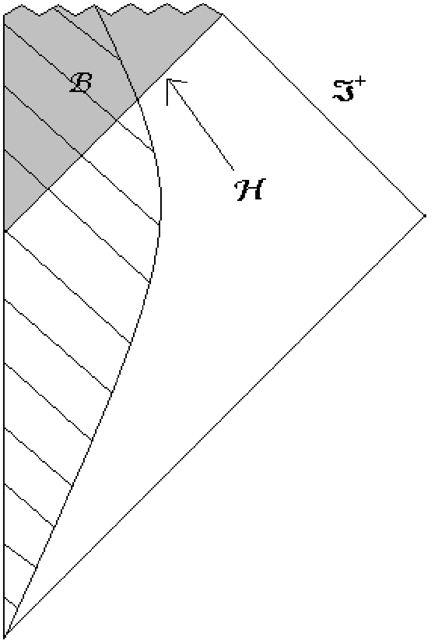
The event horizon of a black hole is then the boundary of . Let us denote the causal past of a set of points and the topological closure of . We have . The (future) event horizon of can then equivalently be defined as
| (3.2) |
i.e. the boundary of the closure of the causal past of . See Fig. 3.1 for an example. The event horizon is a concept defined with respect to the entire causal structure of .
The event horizons are null hypersurfaces with peculiar properties. The development of their properties will allow us to sketch the proof of the area theorem [154] which is concerned with the dynamical evolution of sections of the event horizon at successive times. The area theorem is also called the second law of black hole mechanics because it demonstrates that, under reasonable conditions, the area of the event horizon always increases as does the entropy in classical thermodynamics [64].
1.1 Null hypersurfaces
Let be a smooth function and consider the dimensional null hypersurface , which we denote by . This surface will be the black hole horizon in the subsequent sections. It is a null hypersurface, i.e. such that its normal is null,
| (3.3) |
The vectors tangent to obey by definition. Since is null, itself is a tangent vector, i.e.
| (3.4) |
for some null curve inside . One can then prove that are null geodesics11 1 Proof: Let . We have (3.5) Now, as is null on the horizon, any tangent vector to satisfy . Therefore, and the right-hand side of (3.5) is proportional to on the horizon.
| (3.6) |
where measures the extent to which the parameterization is not affine. If we denote by the normal to which corresponds to an affine parameterization and for some function , then .
According to the Frobenius’ theorem, a vector field is hypersurface orthogonal if and only if it satisfies , see e.g. [243]. Therefore, the vector satisfies the irrotationality condition
| (3.7) |
A congruence is a family of curves such that precisely one curve of the family passes through each point. In particular, any smooth vector field defines a congruence. Indeed, a vector field defines at each point a direction which can be uniquely “integrated” along a curve starting from an arbitrary point.
Since is also defined outside , the normal defines a congruence only null when restricted to . In order to study this congruence outside , it is useful to define a transverse null vector with
| (3.8) |
The normalization is chosen so that if we consider to be tangent to an outgoing radial null geodesic, then is tangent to an ingoing one, see Fig. 3.2. The normalization conditions (3.8) (imposed everywhere, ) do not fix uniquely. Let us choose arbitrarily one such . The extent to which the family of hypersurfaces are not null is given by
| (3.9) |
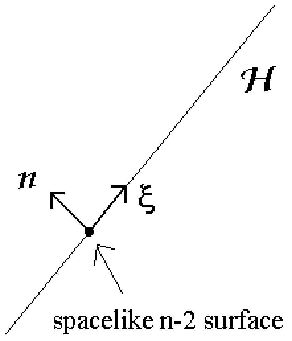
The vectors orthogonal to both and ,
| (3.10) |
span a dimensional spacelike subspace of . The metric can be written as
| (3.11) |
where is a positive definite metric with . The tensor provides a projector onto the spacelike tangent space to .
For future convenience, we also consider the hypersurface orthogonal null congruence with affine parameter that is proportional to on 22 2 We shall reserve the notation for vectors coinciding with on the horizon but which are not null outside the horizon.,
| (3.12) |
The vector field extends outside the horizon while keeping the null property.
1.2 The Raychaudhuri equation
In this section, we shall closely follow the reference [92]. We set out part of the material needed to prove the area law.
Firstly, let us decompose the tensor into the tensorial products of , and spacelike vectors tangent to ,33 3 Proof: Let us first decompose as (3.13) where and , , are spacelike tangents to . Contracting with and using (3.6), we find , . Contracting with , we find . Contracting with , we find finally thanks to (3.3).
| (3.14) |
where the orthogonal projection can itself be decomposed in symmetric and antisymmetric parts
| (3.15) |
The Frobenius irrotationality condition (3.7) is equivalent to 44 4 Proof: We have (3.16) As is defined as a projection with , the equivalence is shown.. The tensor is interpreted as the expansion rate tensor of the congruence while its trace is the divergence of the congruence. Any smooth dimensional area element evolves according to
| (3.17) |
The shear rate is the trace free part of the strain rate tensor,
| (3.18) |
Defining the scalar , one has
| (3.19) |
where was defined in (3.9). Note also that the divergence of the vector field has three contributions,
| (3.20) |
Now, the contraction of the Ricci identity
| (3.21) |
implies the following identity
| (3.22) |
valid for any vector field . The formulae (3.19)-(3.20) have their equivalent for as
| (3.23) |
where the right hand side is expressed in terms of expansion rate and shear rate with respect to the affine parameter . The identity (3.22) becomes
| (3.24) |
where the dot indicates a derivation along the generator. It is the final form of the Raychaudhuri equation for hypersurface orthogonal null geodesic congruences in any dimension.
1.3 Properties of event horizons
As already mentioned, the main characteristic of event horizons is them being null hypersurfaces. In the early seventies, Penrose and Hawking further investigated the generic properties of past boundaries whose event horizons are particular representatives. We shall only enumerate these properties below and refer the reader to the references [155, 235] for explicit proofs. These properties are crucial in order to prove the area theorem.
- 1.
Achronicity property. No two points of the horizon can be connected by a timelike curve.
- 2.
The null geodesic generators of may have past end-points in the sense that the continuation of the geodesic further into the past is no longer in .
- 3.
The generators of have no future end-points, i.e. no generator may leave the horizon.
The second property hold for example for collapsing stars where the past continuation of all generators leave the horizon at the time the horizon was formed. As a consequence of properties 2 and 3, null geodesics may enter but not leave it.
1.4 The area theorem
The area theorem was initially demonstrated by Hawking [154]. We shall follow closely the reviews by Carter [92] and Townsend [235]. The theorem reads as follows.
Theorem 9 (Area law).
If
- (i)
Einstein’s equations hold with a matter stress-tensor satisfying the null energy condition, , for all null ,
- (ii)
The spacetime is “strongly asymptotically predictable”
then the surface area of the event horizon can never decrease with time.
The theorem was originally stated in dimensions but it is actually valid in any dimension .
In order to understand the second requirement, let us recall some definitions. The future domain of dependence of an hypersurface is the set of points in the manifold for which every causal curve through that has no past end-point intersects . The significance of is that the behavior of solutions of hyperbolic PDE’s outside is not determined by initial data on . If no causal curves have past end-points, then the behavior of solutions inside is entirely determined in terms of data on . The past domain of dependence is defined similarly.
A Cauchy surface is a spacelike hypersurface which every non-spacelike curve intersects exactly once. It has as domain of dependence the manifold itself. If an open set admits a Cauchy surface then the Cauchy problem for any PDE with initial data on is well-defined. This is also equivalent to say that is globally hyperbolic.
The requirement (ii) means that there should be a globally hyperbolic submanifold of spacetime containing both the exterior spacetime and the horizon. It is equivalent to say there is a family of Cauchy hypersurfaces , such that is inside the domain of dependence of if .
Now, the boundary of the black hole is the past event horizon . It is a null hypersurface with generator (that is proportional to on ). We can choose to parameterize the Cauchy surfaces using the affine parameter of the null geodesic generator .
The area of the horizon is then the area of the intersection of with . We have to prove that if .
Sketch of the proof:
The Raychaudhuri equation for the null generator reads as (3.24). Therefore, wherever the energy condition holds, the null generator will evolve subject to the inequality
| (3.25) |
except on possible singular points as caustics. It follows that if becomes negative at any point on the horizon (i.e. if there is a convergence) then the null generator can continue in the horizon for at most a finite affine distance before reaching a point at which , i.e. a point of infinite convergence representing a caustic beyond which the generators intersect.
Now, from the third property of event horizons above, the generators cannot leave the horizon. Therefore at least two generators cross at inside and, following Hawking and Ellis (Prop 4.5.12 of [155]), they may be deformed to a timelike curve, see figure 3.3. This is however impossible because of the achronicity property of event horizons. Therefore, in order to avoid the contradiction, the point cannot exist and cannot be negative.

Since (at points where the horizon is not smooth) new null generators may begin but old ones cannot end, equation (3.17) implies that the total area cannot decrease with increasing ,
| (3.26) |
This completes the proof.
In particular, if two black holes with area and merge then the area of the combined black hole have to satisfy
| (3.27) |
The area do not change if on the entire horizon . The black hole is then stationary.
2 Equilibrium states
2.1 Killing horizons
In any stationary and asymptotically flat spacetime with a black hole, the event horizon is a Killing horizon [155]. This theorem firstly proven by Hawking [154] is called the rigidity theorem. It provides an essential link between event horizons and Killing horizons.55 5 The theorem further assumes the geometry is analytic around the horizon. Actually, there exist a counter-example to the rigidity theorem as stated in Hawking and Ellis [155] but under additional assumptions such as global hyperbolicity and simple connectedness of the spacetime, the result is valid [96]. See also [135] for a relaxation of the analyticity hypotheses.
A Killing horizon is a null hypersurface whose normal is a Killing vector
| (3.28) |
This additional property will allow us to explore many characteristics of black holes.
The parameter which we now call the surface gravity of is defined in (3.6). In asymptotically flat spacetimes, the normalization of is fixed by requiring at infinity (similarly, we impose in asymptotically anti-de Sitter spacetimes).
For Killing horizons, the expansion rate , so . Moreover, from (3.20) and (3.28), we deduce . Equation (3.19) then provides an alternative definition for the surface gravity,
| (3.29) |
Contracting (3.6) with the transverse null vector or using the definition (3.9), one has also
| (3.30) |
The Raychaudhuri equation (3.24) also states in this case that
| (3.31) |
because is proportional to on the horizon.
From the decomposition (3.14), the irrotationality condition (3.7) and the Killing property , it can be written
| (3.32) |
where the covector can be fixed uniquely by the normalization . Using (3.30), the last equation can be decomposed in terms of as
| (3.33) |
where satisfy . In particular, it shows that for any spacelike tangent vectors , to , one has .
2.2 Zero law
We are now able to show that the surface gravity is constant on the horizon under appropriate conditions. More precisely,
Theorem 10 (Zero law).
[45] If
- (i)
The spacetime admits a Killing vector which is the generator of a Killing horizon ,
- (ii)
Einstein’s equations hold with matter satisfying the dominant energy condition, i.e. is a non-spacelike vector for all ,
then the surface gravity of the Killing horizon is constant over .
Using the aforementioned properties of null hypersurfaces and Killing horizons, together with
| (3.34) |
which is valid for Killing vectors, one obtains (see [92] for a proof)
| (3.35) | |||||
| (3.36) |
for all spacelike tangent vectors . Now, from the dominant energy condition, is not spacelike. However, the Raychaudhuri equation implies (3.31). Therefore, must be zero or proportional to and .
This theorem has an extension when gravity is coupled to electromagnetism. If the Killing vector field is also a symmetry of the electromagnetic field up to a gauge transformation, , it can also be proven that the electric potential
| (3.37) |
is constant on the horizon. See the discussion before (3.57) for a proof in the case of -form potentials, .
3 First law and Smarr formula
The geometric derivation of the Smarr relation and of the first law of thermodynamics for four-dimensional asymptotically flat black holes is usually based on Komar integrals [45, 90]. Komar integrals are extremely useful since they allow one to easily express the conserved quantities defined at infinity to properties associated with the horizon of the black hole. However, they do not provide a complete and systematic approach to conserved quantities.
Indeed, in order to give the correct definitions of energy and angular momentum, the coefficients of the Komar integrals must be fixed by comparison with the ADM expressions [18, 19], see e.g. discussions in [174, 235]. Moreover, although this approach can be extended to higher dimensional asymptotically flat black holes [197, 138], it generally becomes ambiguous for rotating asymptotically anti-de Sitter black holes [190, 143]. Komar integrals are also not applicable to more exotic black holes as the ones immersed in Gödel spacetimes [146, 43].
The aim of this section is to rederive the first law and the Smarr formula using the Lagrangian charges defined in the preceding part of the thesis, as sketched in [55], without using uniqueness results or assuming spherical horizon topology.
We will first derive the first law and the Smarr formula for Einstein gravity and we will then extend the analysis to gravity coupled to a -form potential and to a scalar field. A proof of the first law for an arbitrary theory of gravity and for non-stationary perturbations will not be developed here. For that analysis, we refer the reader to covariant phase space methods [245, 174].
Following section 5 of Chapter 1, suppose that we have a family of solutions with exact Killing vectors and , , containing stationary and axisymmetric black holes with connected Killing horizon. The generator of a Killing horizon is then a combination of the Killing vectors,
| (3.38) |
where are the angular velocities at the horizon. In what follows, we will only consider one-forms contracted with stationary field variations , i.e. satisfying (1.29),
| (3.39) |
3.1 The first law for Einstein gravity
The differences of energy and angular momenta between two configurations and are defined by
| (3.40) |
Here, the relative sign difference between the definitions of and traces its origin to the Lorentz signature of the metric [174]. We assume that the energy and angular momenta (3.40) are integrable in , i.e. we require that the condition (1.47) or more precisely (2.13) are satisfied for the Killing vectors and , for and for one-forms tangent to the family of solutions .
Assuming that the de Rham cohomology in the solution space vanishes in (vertical) form degree two, the integrability condition ensures that the charge one-forms (1.46) are independent on the path connecting to . The energy and angular momenta are then obtained by integration of (3.40),
| (3.41) |
The equilibrium state version 66 6 There also exists a physical process version, where an infinitesimal amount of matter is send through the horizon from infinity. of the first law for the simple case of pure Einstein gravity can now be stated as [45, 174, 176]
Theorem 11 (First law).
Let and be two slightly different stationary black hole solutions of Einstein’s equations with Killing horizon. The difference of energy , angular momenta and area of the black hole are related by
| (3.42) |
Let us start with Proposition 2 stating the equality of the charge associated with at a spacelike section of the horizon and at infinity,
| (3.43) |
Using (3.40), the left-hand side of (3.43) is given by
| (3.44) |
Using (2.30), the right-hand side of (3.43) may be rewritten as77 7 The minus sign in front of comes from the fact that is Grassman odd and that we use the Grassman even in place of .
| (3.45) |
On the horizon, the integration measure for -forms is given by
| (3.46) |
where is the “angular” measure on and was defined in (3.8). Using the properties of Killing horizons described in section 2, the Komar integral on the horizon can easily be computed as
| (3.47) |
where is the area of the horizon. Now, it turns out that the local geometry around Killing horizons implies the following property
Proposition 12.
| (3.48) |
The computation which is straightforward but lengthly is explicitly done in Appendix C.3 without assuming specific coordinates as in the original derivation [45] and in some later derivations [91, 245]. It would be interesting to find a generalization of this proof for non-stationary perturbations as well.
Using proposition 12, the right-hand side of (3.43) is finally given by
| (3.49) |
as it should and the first law is proven.∎
We can see in this derivation that the first law is a geometrical law in the sense that it relates the geometry of Killing horizons to the geometric measure of energy and angular momenta. Note that the derivation was done in arbitrary dimensions, without hypotheses on the topology of the horizon and for arbitrary stationary variations. The first law also applies in particular for extremal black holes by taking .
3.2 The Smarr formula for Einstein gravity
Let us now derive a formula relating the energy and angular momenta of a black hole with Killing horizon to quantities defined at the horizon. A general derivation can be found in [57].
Let us choose a path , in interpolating between the background and a black hole . It is not assumed that there is a horizon defined for all metrics along the path.
Now, the conserved quantity associated with the Killing generator of the target black hole solution (3.38) is
| (3.50) |
by linearity of in . Because this quantity may be computed on any surface, we can write
| (3.51) |
after having used (3.45). Here, is the black hole horizon and is any surface that may be deformed to the surface at infinity. The Komar integral evaluated on the horizon is given by (3.47). We thus get
| (3.52) |
The claim is that this relation gives the generalized Smarr formula, which becomes the thermodynamical Euler relation, with the standard identifications of temperature as and entropy as . This formula will be applied to Kerr-anti de Sitter black holes and to their flat limit in Chapter 4.
3.3 First law for gravity coupled to a -form potential and a dilaton
The first law of black hole mechanics was initially developed taking into account dust as well as electromagnetic fields [45]. Also, the first law with Yang-Mills fields were studied, e.g., in [224, 137].
Hamiltonian [102], quasilocal [34] as well as covariant phase space methods [209, 210] have investigated the role of -form charges in the first law. The aim of this section published in [101] is to continue the analysis started in section 3 of Chapter 2 by deriving the first law using our methods in a notation taking care of form factors. The first law will be proven for gauge potentials that may be irregular on the bifurcation surface, which is necessary in order to cover e.g. the thermodynamics of black rings [132]. In that respect, the covariant analysis of [209, 210] will be improved.
We will use the observation [137] that a consistent thermodynamics can be done on the future event horizon with diverging potentials if, nevertheless, the potential is regular when pulled-back on the future horizon. Our resulting expression for the first law constitutes a generalization of [137] for -form potentials (also coupled to a scalar field). We will then show in section 4 of Chapter 4 that the potential for the black rings [132] admits a regular pull-back on the future event horizon and can thus be treated by this method. Note that our analysis covers only electric-type charges and not magnetic charges where the potential is necessarily singular on the future event horizon.
We assume as in the previous section that the fields and are stationary black hole solutions with Killing horizon . The variation of energy and angular momenta are defined as the charges associated with the Killing vectors and . We assume that is a solution of (3.1) with . We also require that is a symmetry of the perturbed black hole .
The first law is then a consequence of the equality 88 8 The first law can be straightforwardly generalized to reducibility parameters satisfying with . This simply amounts to add a contribution at infinity and at the horizon.
| (3.53) |
where is a -sphere at infinity. Using the linearity of with respect to , the left-hand side is simply given by . Splitting the right-hand side, we get
| (3.54) |
We showed in the last section that geometric properties of the Killing horizon allow one to express the gravitational contribution into the form
| (3.55) |
Using (2.87), the scalar contribution can be written as
| (3.56) |
which vanishes thanks to the reducibility equations (3.1), assuming the regularity of the scalar field on the horizon.
The contribution of the -form can be computed using the arguments of [138, 102]. The Raychaudhuri equation gives on the horizon. It follows by Einstein’s equations and by the identity that has vanishing norm on the horizon. But as , is tangent to the horizon. has thus the form by antisymmetry of and its pullback to the horizon vanishes. The equation can be written as . Therefore, the pull-back of on the horizon is a closed form.
For , is simply the scalar electric potential at the horizon (3.37). When , the quantity pulled-back on the horizon is the sum of an exact form and an harmonic form . If the horizon has non-trivial cycles , one can define the harmonic forms dual to by duality between homology and cohomology as
| (3.57) |
The harmonic form is then a sum of terms with constant over the non-trivial cycles.
The contribution from the potential contains three terms (2.91). The Komar term (2.89) can be written as
| (3.58) |
where the exact form do not contribute on-shell. We recognize on the right-hand side the conserved form written in (2.94). Let us denote by the integral .
Using (3.46), the contribution reads as
| (3.59) |
The first term of (3.59) nicely combines with the second term of (2.91) into because is constant as a consequence of the hypotheses on the variation. In the second term of (3.59), one can replace by its pull-back on the future horizon. Indeed, decomposing , one sees that the term involving do not contribute because of the antisymmetry of . Therefore, the second term in (3.59) will vanish if is regular and if the pull-back on the future horizon is regular.
Finally, the contribution from the potential on the horizon reduces to
| (3.60) |
as it should to give the first law
| (3.61) |
Chapter 4 Black hole solutions and their thermodynamics
General relativity provides a very elegant classical description of the gravitational interaction. Remarkably, this theory predicts the existence of black holes which satisfy laws analogous to the laws of thermodynamics. In this chapter, we will try to get further insights in the properties of black holes by finding new solutions to gravity coupled to matter fields and by investigating their thermodynamical properties.
In the first section, we will construct new Gödel-type black hole and particle solutions to Einstein-Maxwell theory in 2+1 dimensions with a negative cosmological constant and a Chern-Simons term. These black holes can be seen as B(H)TZ black holes [39, 38] immersed into a Gödel background. We will show that a particular solution is related to the original Gödel universe. The solutions will also be analyzed from the point of view of identifications. On-shell, the electromagnetic stress-energy tensor will be seen to effectively replace the cosmological constant by minus the square of the topological mass and produce the stress-energy of a pressure-free perfect fluid. Finally, the tools developed in the preceding chapters will be used to compute the conserved charges and work out the thermodynamics.
In section 2, we will turn to higher dimensional Kerr-anti-de Sitter black holes. The conserved charges will be obtained by our methods and a generalized Smarr relation which is valid both in flat and in anti-de Sitter backgrounds will be derived. It will be also shown that the charges for higher dimensional Kerr-adS black holes can be correctly computed from the standard Hamiltonian or Lagrangian surface integrals at infinity.
The definition of conserved quantities for Gödel black holes was an open problem in 2004 [146, 183] mainly because the naive application of traditional approaches fails. In section 3, the mass, angular momenta and charge of the Gödel-type rotating black hole solution to five dimensional minimal supergravity [139, 146] will be computed, thereby providing a definition of charges in these unconventional spacetimes. Moreover, a generalized Smarr formula will be derived and the first law of thermodynamics will be verified.
We conclude in sections 4 and 5 with applications of our formalism to black rings and with the definition of energy in plane-waves geometries.
1 Three-dimensional Gödel black holes
Exact solutions of higher dimensional gravity and supergravity theories play a key role in the development of string theory. Recently, a Gödel-like exact solution of five-dimensional minimal supergravity having the maximum number of supersymmetries has been constructed [139]. As its four-dimensional predecessor, discovered by Gödel in 1949 [149], this solution possesses a large number of isometries. It can be lifted to higher dimensions and has recently been extensively studied as a background for string and M-theory, see e.g. [70, 152].
The Gödel-like five-dimensional solution found in [139] is supported by an Abelian gauge field. This gauge field has an additional Chern-Simons interaction and produces the stress-energy tensor of a pressureless perfect fluid. Since a Chern-Simons term can also be added in three dimensions, it is a natural question to ask whether a Gödel like solution exists in three-dimensional gravity coupled to a Maxwell-Chern-Simons field.
Actually, there is a stronger motivation to look for this kind of solutions of three-dimensional gravity. The reason is that the original four-dimensional Gödel spacetime is already effectively three dimensional, see e.g. [155]. In fact, the metric has as direct product structure where satisfies a purely three-dimensional Einstein equation.
The goal of this section, published as an article in [43] with M. Banados, G. Barnich and M. Gomberoff, is twofold. On the one hand we will show that the three-dimensional factor of the Gödel spacetime and its generalizations [206] are exact solutions of the three-dimensional Einstein-Maxwell-Chern-Simon theory described by the action,
| (4.1) |
The stress-energy tensor of the perfect fluid will be fully generated by the gauge field , in complete analogy with the five-dimensional results reported in [139].
Our second goal deals with Gödel particles and black holes. Within the five-dimensional supergravity theory, rotating black hole solutions on the Gödel background have been investigated in [165, 146, 72, 147, 62, 183, 148, 59, 109]. It is then natural to ask whether the three-dimensional Gödel spacetime can be generalized to include horizons. This is indeed the case and a general solution will be displayed.
The conserved charges - mass, angular momentum and electric charge - will be computed for these solutions and the first law for the three-dimensional black holes, adapted to an observer at rest with respect to the electromagnetic fluid will be derived. We then show how to adapt this first law in order to compare with the one for adS black holes in the absence of the electromagnetic fluid.
In parallel to this work, three-dimensional black hole solutions with naked closed time-like curves have also been obtained from exact marginal deformations of the WZW model [122]. Gödel black hole solutions can thus be promoted to exact string theory backgrounds. During the writing of this thesis, the supersymmetric extension of the action (4.1) has been constructed in [44]. It turns out that the three-dimensional Gödel solution preserves one half of the supersymmetries.
1.1 Introduction
Let us now briefly discuss the general structure of the stress-energy tensor of Maxwell-Chern-Simons theory. The original Gödel geometry is a solution of the Einstein equations in the presence of a pressureless fluid with energy density and a negative cosmological constant such that . Equivalently, it can be viewed as a homogeneous spacetime filled with a stiff fluid, that is, and vanishing cosmological constant.
In (2+1)-spacetime dimensions, an electromagnetic field can be the source of such a fluid. To see this it is convenient to write the stress-energy tensor in terms of the dual field ,
| (4.2) |
In any region where the field is timelike, the electromagnetic field behaves as a stiff fluid with
| (4.3) |
If Gödel’s geometry is going to be a solution of the Einstein-Maxwell system, then must be a constant. Moreover in comoving coordinates, in which , must be a constant vector pointing along the time coordinate. One can easily see that such a solution does not exist. In fact, the Maxwell equations for this solution,
| (4.4) |
imply in these coordinates that which cannot be achieved for Gödel. If the electromagnetic field acquires a topological mass , however, Maxwell’s equations (4.4) will be modified by the addition of the term . In that case, the timelike, constant, electromagnetic field is, as we will see below, a solution of the coupled Einstein-Maxwell-Chern-Simons system, and the geometry is precisely that of Gödel.
1.2 Topologically massive gravito-electrodynamics
We start by reviewing the main properties, relevant to our discussion, of the four-dimensional Gödel spacetimes [149, 206, 211]. These metrics have a direct product structure with three-dimensional factor given by
| (4.5) | |||||
The original solution discovered by Gödel corresponds to . Furthermore, it was pointed out in [206] that the property of homogeneity and the causal structure of the Gödel solution also hold for and independent, provided that , the limiting case corresponding to anti-de Sitter space.
The three-dimensional metric (4.5) has 4 independent Killing vectors, two obvious ones, and , and two additional ones,
| (4.6) | |||||
| (4.7) | |||||
which span the algebra . Finally, the metric (4.5) satisfies the three dimensional Einstein equations,
| (4.8) |
for all values of , and we see that plays the role of a negative cosmological constant.
Note that a solution to Einstein’s equations in dimensions can be lifted to a solution in dimensions through the addition of a flat direction if the additional components of the stress-energy tensor are chosen as and . For the solutions (4.5), and vanishes, as it should, for the original Gödel solution.
Our first goal is to prove that (4.5) can be regarded as an exact solution to the equations of motion following from (4.1).
To this end, we need to supplement (4.5) with a suitable gauge field which will provide the stress-energy tensor (right hand side of (4.8)). Consider a spherically symmetric gauge field in the gauge ,
| (4.9) |
Inserting this ansatz for the gauge field into the equations of motion associated to the action (4.1), and assuming that the metric takes the form (4.5), one indeed finds a solution for and . Moreover, the two parameters entering in (4.5) become related to the coupling constants and as
| (4.10) |
With this parameterization, the Gödel sector is determined by , with corresponding to anti-de Sitter space. For future convenience, we shall write the solution in terms of a new radial coordinate defined by
| (4.11) |
Explicitly, the metric and gauge field are given by,
| (4.12) | |||||
| (4.13) |
From now on, we always write and in terms of and using (4.10). The general solution for involves the addition of arbitrary constant terms along and in (4.13). At this stage, we choose the constant in to be zero. We will come back to this issue when we discuss black hole solutions below. A constant term in is not allowed, however, if one requires to be regular everywhere. Indeed, near , the spacelike surfaces of (4.12) are in polar coordinates, the radial coordinate in (4.12) being the square root of a standard radial coordinate over , and thus must vanish at because the 1-form is not well defined there.
The gauge field (4.13) is also invariant under the isometries of (4.5), up to suitable gauge transformations: for each Killing vector there exists a function such that
| (4.14) |
In this sense, the Killing vectors of (4.5) are lifted to gauge parameters that leave the full gravity plus gauge field solution invariant. The generalized Gödel metric (4.12) together with the gauge field (4.13) define a background for the action (4.1) with 4 linearly independent symmetries of this type. We shall now use these symmetries in order to find new solutions describing particles and black holes.
1.3 Gödel particles:
We have proven in the previous section that the Gödel metric can be regarded as an exact solution to action (4.1). The associated gauge field (4.13) is however real only in the range . We consider in this section the case and introduce particle-like objects on the background (4.12) by means of spacetime identifications.
Gödel Cosmons
Identifications in three-dimensional gravity were first introduced by Deser, Jackiw and t’Hooft [117, 118] and the resulting objects called “cosmons”. In the presence of a topologically massive electromagnetic field, cosmons living in a Gödel background may also be constructed along these lines.
Take the metric (4.12) and make the following identification along the Killing vectors and
where are real constants. If this procedure will turn the spatial plane into a cone. The cosmon lives in the tip of this cone, and its mass is related to and (see below). The time-helical structure given by will provide angular momentum.
To analyze the resulting geometry it is convenient to pass to a different set of coordinates,
| (4.15) | |||||
where the above identification amounts to
| (4.16) |
Also, the new time flows ahead smoothly, that is, it does not jump after encircling the particle. Inserting these coordinates into (4.12), and erasing the primes, we find the new metric
| (4.17) | |||||
For fixed and , the new constants and are given by
| (4.18) | |||
| (4.19) |
These constants will be shown to be related to the mass and angular momentum respectively.
Since under (4.15) scales with while with we see that the -dependent part of gauge field (4.13) is invariant under (4.15). However, the manifold now has a non-trivial cycle, and it is not regular at the point invariant under the action of the Killing vector whose orbits are used for identifications. Explicitly, which corresponds to before the shift of in (4.15). This means that one can now add a constant piece to . The new gauge field becomes
| (4.20) |
The constant will be identified below as the electric charge of the particle sitting at .
Horizons, Singularities and Time Machines
Distinguished places of the geometry (4.17) may appear on those points where either or vanishes. The vanishing of indicates that changes sign and hence closed timelike curves (CTC) appear. On the other hand, the vanishing of indicates the presence of horizons, as can readily be seen by writting (4.17) in ADM form.
The function in (4.17) is an inverted parabola, and, it will have two zeros, say and whenever
| (4.21) |
We must require this condition to be fulfilled in order to have a “normal” region where is spacelike. The boundary of the normal region are two spacelike surfaces, the velocity of light surfaces (VLS) at and (assume ). These surfaces are perfectly regular as long as there, which is indeed the case for the metric (4.17), when .
On the other hand, it is direct to see from (4.17) that
| (4.22) |
Since is positive in the normal region, there are no horizons there and is positive in that region. This means that, if any, both zeros of are on the same side of the normal region. The sides in which no zero of are present are analog to the Gödel time machine, an unbounded region, free of singularities, where is timelike. If , the roots of are smaller than the roots of . Without loss of generality, we can restrict ourselves to this case because the solutions parametrized by are related to those with by the change of coordinates , .
The condition for “would be horizons” is
| (4.23) |
As depicted in Fig. 4.1, once one reaches the largest root of , the manifold comes to an end. Indeed, the signature of the metric changes as one passes . This can be seen by putting the metric in ADM form (see (4.50) below). Note that in this case, given , there is a unique satisfying (4.18)-(4.19).
Using then , with the smallest root of and , one finds near ,
| (4.24) |
This means that the spacetime has a naked singularity at , which is the analog of the one found in the spinning cosmon of [117, 118].
Alternatively, as proposed originally in [109] for the case where the would be horizon is inside the time machine, one can periodically identify time with period . This leads to having CTC’s lying everywhere, including the normal region.

1.4 Gödel black holes
The sector
We have shown in Sec. 1.2 that the metric (4.5) can be embedded as an exact solution to the equations of motion derived from (4.1). The necessary gauge field, given in (4.13) is, however, real only in the range . As we mentioned in Sec. 1.2, the gauge field (4.13) represents the most general static spherically symmetric solution, given the metric (4.5) (or, in the new radial coordinate, (4.12)). This means that if we want to find a real gauge field in the range we need to start with a different metric. The goal of this section is to explore the other sector, , where black holes will be constructed.
Starting from the metric (4.12) and gauge field (4.13) it is easy to construct a new exact solution which will be real in the range . Consider the following (complex) coordinate changes 11 1 An equivalent way to do this transformation without introducing the imaginary unit is by the following sequence of coordinate transformations (and analytic continuations) acting on (4.12): , , , and the same for . acting on (4.12) and (4.13): , , and . The new metric and gauge field read,
| (4.25) | |||||
| (4.26) |
Several comments are in order here. First of all, the intermediate step of making some coordinates complex is only a way to find a new solution. From now on, all coordinates are defined real, and, in that sense, the fields (4.25) and (4.26) provide a new exact solution to the action (4.1) which is real in the range .
Second, in the original metric (4.12), the coordinate was constrained by the geometry to have the range . This is no longer the case in the metric (4.25). The 2-dimensional sub-manifold described by the coordinates does not have the geometry of near anymore; the coordinate is thus not constrained to be compact, and in principle it should have the full range
| (4.27) |
The reason that in (4.25) is not constrained by the geometry is that the component of the metric (4.25) changes sign as we approach . This is an indication of the presence of a horizon, although this surface is not yet compact.
Finally, it is worth mentioning that the metrics (4.25) and (4.12) are real and are related by a coordinate transformation, so that all local invariants involving the metric alone have the same values. However, as solutions to the Einstein-Maxwell equations, they are inequivalent. Indeed, the diffeomorphism and gauge invariant quantity changes sign when going from (4.12)-(4.13) to (4.25)-(4.26). This is different from the pure anti-de Sitter case where particles and black holes are obtained by identifications performed on the same background.
The Gödel black hole
Let us go back to (4.25) and note that the function vanishes at . In order to make the surface a regular, finite area, horizon we shall use the Killing vector of (4.25) to identify points along the coordinate. In this case, has a non-compact orbit and identifications along it does not produce a conical singularity, but a “cylinder”. More generically, we may proceed in analogy with the cosmon case and identify along a combination of both and so that
so that the resulting geometry will also carry angular momentum. We again pass to a different set of coordinates,
| (4.28) | |||||
| (4.29) | |||||
| (4.30) |
so that the new angular coordinate is identified in , and the time flows ahead smoothly.
The new metric reads (after erasing the primes),
| (4.31) | |||||
As for the particles analyzed in the previous section, for given , we define new constants and according to
| (4.32) | |||
| (4.33) |
Again, these constants will be related below to the mass and the angular momentum and without loss of generality, we can limit ourselves to the case .
In the new coordinates, the electromagnetic potential takes the form , where
| (4.34) |
The constant is arbitrary because, once again, the nontrivial topology allows the addition of an arbitrary constant in . It is worth stressing that if was not compact, then and would be trivial constants. It also follows that the Killing vectors of (4.25) have the same form as those of (4.12), but with the trigonometric functions and replaced by hyperbolic ones. Again, these vectors do not survive after the identifications.
Horizons, Singularities and Time Machines
We now proceed to analyze the metric in the same way we did in the preceding section. Again we have a condition for having a normal region, which, in this case reads
| (4.35) |
The functions and now behave as in Fig. 4.2.

Note that
| (4.36) |
and therefore horizons may only exist in the normal region of positive . Note, however, that for horizons to exist we must require
| (4.37) |
If this requirement is fulfilled, we get two horizons inside the normal region, and , which coincide in the extremal case. The whole normal region is in fact an ergoregion because is spacelike everywhere. Again, for given , one can then find a unique solution satisfying (4.32)-(4.33).
Following Carter [91], the metric and the gauge field can be made regular at both horizons by a combined coordinate and gauge transformation. Indeed, if
the black hole metric can be written as
| (4.38) |
The analog of ingoing Eddington-Finkelstein coordinates are the angle and the time defined by , , giving the regular metric
| (4.39) |
With given by (4.34), the dependent gauge transformation , where gives the regular potential whose norm is zero.
Outgoing Eddington-Finkelstein coordinates are defined by , . The metric then takes also the form (4.39) with and replaced by and and the potential can be regularized by .
The null generators of the horizons are . The associated ignorable coordinates which are constant on these null generators are then given by
| (4.40) |
Kruskal type coordinates are obtained by defining
| (4.41) | |||||
| (4.42) |
where
In these coordinates, the metric is manifestly regular at the bifurcation surfaces,
| (4.43) | |||||
with given implicitly by
| (4.44) |
In Kruskal coordinates, the gauge field (4.34) becomes
| (4.45) | |||||
The potential can be regularized at by the transformations
| (4.46) | |||||
In the original coordinates, however, the parameters of these transformations explicitly involve the angle , and, as explicitly shown below, they change the electric charge. In order to avoid this, one can add a constant piece proportional to , so that
| (4.47) |
In the original coordinates, the gauge parameter is now a linear function of alone,
| (4.48) |
According to the definition given below, such a transformation does not change the charges.
In the published paper [43], a naive Carter-Penrose diagram for these black holes was drawn. This diagram, however, is premature in view of the two following issues that have still to be addressed: namely, the clarification of the global topology of these spacetimes, and the existence of a conformal completion. These considerations are left for further work.
1.5 Vacuum solutions
In the case the gauge field vanishes and the Gödel metric (4.12) reduces to the three-dimensional anti-de Sitter space (to see this, do the coordinate transformations and ). This means that the identifications in this case yield the usual three-dimensional black holes, and conical singularities.
1.6 The general solution
Reduced equations of motion
We have seen in previous sections that the Gödel metrics (4.5) and (4.25), as well as the corresponding quotient spaces describing particles and black holes, can be regarded as exact solutions to the action (4.1).
We have distinguished three cases according to the values of the dimensionless quantity . Our purpose in this section is to write a general solution which will be valid for all values of . We shall now construct the solution by looking directly at the equations of motion. It is useful to write a general spherically symmetric static ansatz in the form [98, 14]
| (4.49) |
where are functions of only. This ansatz can also be written in the “ADM form”,
| (4.50) |
This confirms that the function
| (4.51) |
controls the existence of horizons. Note that for all , the determinant of this metric is For the gauge field, we use the radial gauge , and assume that and depend only on the radial coordinate,
| (4.52) |
In this parametrization, Einstein’s equations take the remarkably simple form,
| (4.53) | |||||
where primes denote radial derivatives. Maxwell’s equations reduce to
| (4.54) |
Before we write the solution to these equations, we make some general remarks on the structure of the stress-energy tensor associated to topologically massive electrodynamics. As we pointed out in the introduction, we will seek for solutions with a constant electromagnetic field . Hence, we will only consider potentials which are linear in . In this case, Eqs. (4.54) are
| (4.55) |
We now multiply the first by and the second by , then we subtract them to obtain
In the last step we have used Eq. (4.55). This implies that, if then . By properly manipulating Eqs. (4.55) we see that this result is also valid if but , and therefore is it true as long as the electromagnetic field does not vanish. Now we insert this in the last equation in (4.53), and obtain,
| (4.56) | |||||
This equation tells us that when the topological mass is greater (smaller) than the negative cosmological constant , the theory only supports timelike (spacelike) constants fields. Therefore, for the generalized Gödel spacetimes (4.5), we will need a topological mass . In the other region, the constant electromagnetic field will describe a tachyonic perfect fluid. Anyway, as we will see below, it is this region in which black hole solutions are going to exist.
The solution
By direct computation one can check that equations (4.53)-(4.54) are satisfied by the field
| (4.57) | |||||
where
| (4.58) |
The parameters , and are integration constants with a physical interpretation as they will be identified with mass, angular momentum and electric charge below. The arbitrary constant on the other hand will be shown to be pure gauge. For later convenience, it is however useful to keep it along and not restrict ourselves to a particular gauge at this stage. This will be discussed in details Sec. 1.7.
In the sector , the solution is real only for negative. These are the Gödel particles, i.e., the conical singularities, discussed in Sec. 1.3. The metric (4.17) is recovered when and the change of variables , is performed. For the special values and , which correspond to the trivial identification , in Sec. 1.3, the conical singularities disappear and we are left with the Gödel universes (4.12), used for the identifications producing the cosmons.
When , has to be positive. The black hole metrics (4.31) of Sec. 1.4 are recovered when and , . For and , they reduce to the solution (4.25) from which the black holes have been obtained from non-trivial identifications.
By construction, the electromagnetic stress-energy tensor for the solutions (4.57) takes the form
| (4.59) | |||||
| (4.60) |
where the unit tangent vector of the fluid is . For , the effect of the electromagnetic field can be taken into account by replacing the original cosmological constant by the effective cosmological constant and introducing a pressure-free perfect, ordinary or tachyonic, fluid with energy density . From this point of view, the Chern-Simons coupling transmutes into a cosmological constant. For , the fluid flows along timelike curves while for , the fluid is tachyonic.
When , the fluid disappears, the stress-energy tensor vanishes and the solution is real for . The metric (4.57) reduces to the BTZ metric [39], as can be explicitly seen by transforming to the standard frame that is non-rotating at infinity with respect to anti-de Sitter space,
| (4.61) |
As will be explained in more details below, in the rotating frame that we have used, the energy and angular momentum are and respectively, while they become and in the standard non-rotating frame.
Regular black holes have the range (see Fig. 4.4)
| (4.62) |
Note that the solution still possess a topological charge . It has been discussed in more details in [14].
When , the limit can be taken smoothly in the coordinates , in which the solution becomes
| (4.63) | |||||
where .
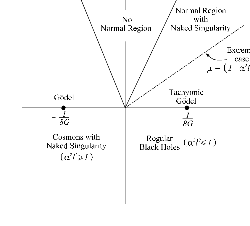

1.7 Conserved charges
Angular momentum, electric charge and energies
The charge differences between a given solution and an infinitesimally close one were computed in section 4 of Chapter 2.
Particularizing to three dimensions and contracting the vertical one-forms with variations satisfying the reducibility equations
the (1,1)-forms can be simplified as
| (4.67) |
with22 2 The minus sign of in front of as compared to (2.10) comes from the fact that is Grassmann even () while is Grassmann odd ().
| (4.68) |
where
| (4.69) |
is the Komar 1-form and
The electromagnetic contribution is33 3 The same remark as the preceding footnote applies to the term as compared to (2.91).
| (4.70) |
where
| (4.71) | |||||
| (4.72) |
The Chern-Simons term contributes as
| (4.73) |
For generic metrics and gauge fields of the form (4.57), the general solution of (1.7) is a linear combination of , and . These basis elements are associated to infinitesimal charges as follows,
| (4.74) |
where the contribution proportional to in and originate from the Chern-Simons term through (4.73). The conserved charges associated with , are thus manifestly integrable. We choose to associate the angular momentum to so that its value be algebraically independent of . If one takes as basis element instead of , one gets a third integrable conserved charge equal to .
The integrated charges computed with respect to the background and associated to , and are the mass, the angular momentum and the total electric charge respectively,
| (4.75) |
Note that even though the metric and gauge fields in (4.57) become singular at the background , we can see from the form (4.63) that this is just a coordinate singularity.
The parameter is pure gauge because the variation is not present in the infinitesimal charges (1.7). Note however that appears explicitly in the definition of the mass by associating it with the basis element . It is only in the gauge , that the mass is associated with the time-like Killing vector . This definition ensures in particular that the mass of the black hole does not depend on the gauge transformations (4.48) needed to regularize the potential on the bifurcation surfaces.
In order to compare with standard adS black holes, one has to compute the mass in the frame (4.61) instead of using the rest frame for the fluid. The conserved charge associated with is now given by
| (4.76) |
which coincides with the conventional definition of the mass for the BTZ black holes.
Horizon and first law - General derivation
When it exists, the outer horizon is located at , the largest positive root of . In the following, a subscript on a function means that it is evaluated at . The generator of the horizon is given by , where the angular velocity of the horizon has the value
| (4.77) |
where denotes the sign of . The first law can be derived by starting from
| (4.78) | |||||
The first term on the right-hand side was computed in section 3 of Chapter 3 with as final result
| (4.79) |
where the total electric potential is given by
| (4.80) |
The surface gravity is given by
| (4.81) |
and the proper area by
| (4.82) |
Note that the choice of signs in the definition of electric charge and angular momentum were made so that the first laws appear in the conventional form (4.79).
Horizon and first law - Explicit values and discussion
We have
| (4.83) |
so that
| (4.84) |
In order to explicitly verify the first law (4.79), we start by showing that . We need to verify that
| (4.85) |
Using the explicit expressions for the components of , this equation reduces to
| (4.86) |
Taking into account together with , this equality can then easily be checked using , , implying . Since , the first law reduces to
| (4.87) |
which can be explicitly checked using (4.84).
In particular, the first law (4.79) can be evaluated in the gauge where the potential is regular on the horizon . Because the two forms (4.31) and (4.57) of the black hole solution are related by the change of coordinates , , the gauge (4.48) now corresponds to
| (4.88) |
This amounts to the choice in (4.57). It follows that and that the vector associated to is proportional to on the horizon.
The first law adapted to the energy is obtained by changing to in (4.79). This form of the first law reduces to the standard form for 3 dimensional adS black holes (with or without topological charge) when .
Finally, we note that the first law (4.79) applies both to the outer event horizon of a black hole in the normal region and to the horizon at of a cosmon, when time is identified with real period .
2 Kerr-anti-de Sitter black holes
The general Kerr-anti-de Sitter metrics in arbitrary spacetime dimensions were found recently in [145], generalizing the results of Myers and Perry [197] to non-vanishing cosmological constant.
As has been emphasized in [143], not even in four dimensions do all authors obtain the same expression for the energy of Kerr-adS black holes. Much worse, some of these expressions are in disagreement with the first law. In [143], Gibbons et al. computed the energy of such black holes indirectly by integrating the first law. In [115], the mass and energy have been computed directly by using the BKL superpotentials [181]. In a completed version of their paper, Gibbons et al. then have also computed the energy directly by using the Ashtekar-Magnon-Das definition [24, 30].
In this section, published in [57], we compute the conserved charges - mass and angular momenta - for the Kerr-adS black holes by using the surface integrals developed in the preceding chapters and we find agreement with the results of [143, 115]. We also show explicitly that, in this case, the surface integrals integrated along a path of solutions reduce to the standard Lagrangian [2] or Hamiltonian [159, 158] surface integrals at infinity.
Finally, we give a detailed and geometric derivation of the generalized Smarr relation for the higher dimensional Kerr-adS black holes, in the continuation of section 3.2 of Chapter 3. The derivation can also be applied straightforwardly to asymptotically flat black holes in the limit of vanishing cosmological constant.
2.1 Description of the solutions
The general Kerr anti-de Sitter metrics in dimensions44 4 In this section we shall use the notations of [143] except the spacetime dimension denoted by and the indices , which run from 1 to , while run from 1 to . When , . We also use where were obtained in [145, 144]. They have independent rotation parameters in orthogonal 2-planes. Gibbons et al. start from the dimensional anti-de Sitter metric in static coordinates,
| (4.89) |
with . They then consider the change of variables to Boyer-Linquist spheroidal coordinates . These coordinates depend on arbitrary parameters and are defined by
| (4.90) |
Note that for later convenience, we have renamed the variables as already at this stage. The anti-de Sitter metric then becomes
| (4.91) | |||||
where
| (4.92) | |||||
| (4.93) |
In the coordinates , the Kerr-adS solutions , depending on parameters , are related to the AdS metric as follows:
| (4.94) |
as can be directly verified by comparing with equation (4.2) of [143]. In these coordinates, defining the metric deviations through
| (4.95) |
and using , , it is straightforward to see that
| (4.96) |
with , while all other components of vanish.
The Killing vectors of the Kerr metric are given in coordinates and by
| (4.97) |
2.2 Mass and angular momenta
Surface charges
The -forms for general relativity were computed in section 2 of Chapter 2. For exact Killing vectors of the metric and for variations contracted with , one can simplify the expression (2.10) with (2.27), (2.28) and (2.29) to
| (4.98) |
where .
The conserved charges for the family of solutions (4.94) are then obtained as outlined in section 5 of Chapter 1. Let with denote a one parameter family of solutions to Einstein’s equations interpolating between the anti-de Sitter background and the Kerr-adS solution . For , can be obtained by replacing by in (4.94). Let be a Killing vector field for this family55 5 We consider only vectors that do not vary along the path ., , and be the tangent vector to in solution space. The charge associated with is then defined as
| (4.99) |
and depend only on the homology class of . We will check below that the charge associated with the Killing vectors (4.97) are integrable. Because the space of parameters of the solutions (4.94) has trivial topology, it will imply that the charges (4.99) do not depend on the particular path chosen. More explicitly, we have
| (4.100) | |||
| (4.101) |
The total energy of spacetime is defined to be , while the total angular momenta are . Because the charges only depend on the homology class of , one can evaluate them on the sphere at infinity in order to allow their comparison with the usual Lagrangian and Hamiltonian surface charges at infinity [2, 159, 158].
Useful integrals
Let us define the spheroid in coordinates by , . Using given explicitly in equation (A.9) of [143] and expressing as a function of the remaining , , it is straightforward to show that
| (4.102) |
where is the volume of the unit sphere, given explicitly for instance in (4.9) of [143].
Similarly,
| (4.103) |
This identity has been verified using Mathematica up to . We suppose it holds for higher .
Angular momenta
Because is tangent to , the charge (4.100) reduces to the standard expression for the angular momenta in terms of Komar integrals:
| (4.104) |
and is path independent. Explicitly, one gets
| (4.105) | |||||
Here, the Komar integral evaluated for the background does not contribute because . The result agrees with the one given in [143].
Mass
In order to compute the mass, we evaluate (4.100) with on . We have
| (4.106) |
Let decompose the metric as . The asymptotic behavior (4.96) of implies that . Hence, in the expansion of the inverse metric
| (4.107) |
only the first two terms will contribute to integral (4.106), since the following terms fall off faster and keeping only the first two terms will give finite contributions, as we will show. Injecting this expansion into (4.106), one gets terms that are at most quadratic in . The terms of order will cancel, while the terms quadratic in can directly be shown not to contribute. Hence, only terms linear in will contribute to (4.106) with the result
| (4.108) | |||||
The integral defined in (4.101) reduces to
| (4.109) |
where (and indices are lowered and raised with and its inverse). Note that the equality implies . From the definition of the metric (4.94), one can see that
| (4.110) |
where is the adS metric and is defined in (4.95). Now, as the leading terms in expression (4.110) give finite contributions to the integral (4.109), as we will show below, the sub-leading terms will not contribute. Expanding as in (4.107), we get
| (4.111) |
where the indices are raised with and where indicates that the sub-leading terms in equation (4.110) have been dropped. Again, we will show below that the first two terms of (4.111) give finite contributions to the integral (4.109). As the following terms in (4.111) fall off faster, we can safely ignore them in the computation. If we now expand the expressions , and in the integrand in terms of and of , we obtain after some work that
| (4.112) |
where all the dependence in appear only in the vanishing term . As a consequence, the integral (4.109) does not depend on the path.
Comparison with alternative surface charges
Actually, in (4.112) and because , we showed that
| (4.115) |
with because all terms of which are of order or higher in an expansion according to of vanish when one approaches the boundary at infinity. Hence, we have shown that at , the mass can be computed using
| (4.116) |
with and where the -form is given in (4.98). Moreover, as shown in (4.104), the same relation (4.116) hold for replaced by the Killing vectors .
Now, because of the equivalence of expression (4.98) with (2.24) proven in section 2.1 of Chapter 2, the conserved charge (4.116) for is exactly the Abbott-Deser surface charge [2] associated with the Killing vector of the anti-de Sitter background .
Moreover, using the results of section 2.3 of Chapter 2, one can write the conserved charge (4.116) related to the Killing vector , of the background in the hamiltonian form derived in [159, 158],
| (4.117) | |||
| (4.118) |
with and . In this expression, , denotes the spatial background three metric, which is used, together with its inverse to lower and raise indices, is the associated covariant derivative, are the conjugate momenta, , with and , with the lapse function.
Finally, the charge derived in [181] is defined on the sphere at infinity as
| (4.119) | |||||
with
| (4.120) |
This expression coincides to first order in with where the one-form is given in (4.98) as can easily be seen by using . Hence, the BKL expression gives the same results as the charge because the boundary conditions are such that the terms quadratic and higher in vanish asymptotically.
2.3 Generalized Smarr relation
The Smarr relation is given in general relativity by the expression (3.52). Let us now evaluate the terms on its right-hand side.
The integral evaluated on the surface , where the horizon radius is the largest root of , is given by
| (4.121) |
Note that this integral vanishes in Minkowski space .
In Kerr-adS spacetimes, the Komar integrand of a Killing vector is not closed. Indeed, using the equations of motion , we have
| (4.122) | |||||
| (4.123) |
Because , we have . It then follows from the definition of (4.101) and from the identity that . We thus can move the integral on the horizon back out to infinity,
| (4.124) |
The first term on the right hand side has already been computed in (4.113), while the second term vanishes because does not vary along the path and is tangent to .
We can now write the Smarr formula (3.52) as
| (4.125) |
in complete agreement with the results obtained by Euclidean methods in [143].
3 Gödel black holes in supergravity
Black hole solutions in supergravity theories have attracted a lot of interest recently for two main reasons. On the one hand, higher dimensional supersymmetric theories play a prominent role in the effort of unifying gravity with the three microscopic forces and on the other hand, black hole solutions are preferred laboratories to study effects of quantum gravity.
Among the supersymmetric solutions of five dimensional minimal supergravity [139], a maximally supersymmetric analogue of the Gödel universe [149] has been found. This solution can be lifted to 10 or 11 dimensions (see also [237]) and has been intensively studied as a background for string and M-theory, see e.g. [70, 152].
Black holes in Gödel-type backgrounds have been proposed in [165, 146, 166, 72, 62]. Usually, given new black hole solutions, the conserved charges are among the first properties to be studied, see e.g. [197, 138, 143]. Indeed, they are needed in order to check whether these solutions satisfy the same remarkable laws of thermodynamics as their four dimensional cousins [45, 90].
The computation of the mass, angular momenta and electric charge of the Gödel black holes was an open problem in 2004, mentioned explicitly in [146] with partial results obtained in [183] because the naive application of traditional approaches fails. The aim of the computation below, published as a paper in [59], is to solve this problem for the five dimensional spinning Gödel-type black hole [146] and to derive both the generalized Smarr formula and the first law.
In what follows, we consider the bosonic part of minimal supergravity in dimensions described by the Lagrangian (2.97) with and .
The Gödel-type solution [237, 139] to the field equations is given by
| (4.127) | |||||
where the Euler angles belong to the intervals , , and where . It is the reference solution with respect to which we will measure the charges of the black hole solutions of [146] that we are interested in. These latter solutions can be written as
| (4.128) | |||
They reduce to the Schwarzschild-Gödel black hole when , whereas the five dimensional Kerr black hole with equal rotation parameters is recovered when .
Consider a path in solution space joining the solution to the background . Whenever two dimensional closed hypersurfaces and can be chosen as the only boundaries of an dimensional hypersurface , the charges defined by
| (4.129) |
where are reducibility parameters (4) do not depend on the hypersurfaces or used for their evaluation. Furthermore, the integrability conditions satisfied by , as shown in the computations below, and the absence of topological obstructions imply that these charges do not depend on the path, but only on the initial and the final solutions.
We choose to integrate over the surface defined by , while the path interpolating between the background Gödel-type universe and the black hole is obtained by substituting by in (4.128), with . Because for all , the mass
| (4.130) |
of the black hole comes from the gravitational part (2.10) only
| (4.131) | |||||
Unlike the five dimensional Kerr black hole [197, 138], the mass of which is recovered for , we also see that the rotation parameter brings a new contribution to the mass with respect to the Schwarzschild-Gödel black hole.
Note that the integral over the path is really needed here in order to obtain meaningful results, because the naive application of the Abbott-Deser (2.24), Iyer-Wald (2.10) or Regge-Teitelboim (2.46) expressions evaluated on gives as a result
| (4.132) |
which, as pointed out in [183], diverges for large . A correct application consists in using these expressions to compare the masses of infinitesimally close black holes, i.e., black holes with as compared to black holes with . Indeed, , with given by the r.h.s of (4.131), which is finite and independent as it should since . Finite mass differences can then be obtained by adding up the infinitesimal results. This procedure is for instance also needed if one wishes to compute in this way the masses of the conical deficit solutions [116] in asymptotically flat 2+1 dimensional gravity.
Because our computation of the mass does not depend on the radius at which one computes, one can consider, if one so wishes, that one computes inside the velocity of light surface. Similarly, if one uses this method to compute the mass of de Sitter black holes, one can compute inside the cosmological horizon, and problems of interpretation, due to the fact that the Killing vector becomes space-like, are avoided.
The expression for the angular momentum
| (4.133) |
reduces to
| (4.134) |
Using (2.27) and (2.102), we get
| (4.135) |
while the angular momenta for the other 3 rotational Killing vectors [146] vanish.
The electric charge picks up a contribution from the Chern-Simons term and is explicitly given by (2.105),
| (4.136) |
In particular, it vanishes for the Schwarzschild-Gödel black hole.
Generalized Smarr formula and first law.
Consider a stationary black hole with Killing horizon determined by , where denotes the time-like Killing vector, the angular velocities of the horizon and the axial Killing vectors and let , . As discussed in section 3.2 of Chapter 3, the definition of and the charges imply
| (4.137) |
where is a dimensional surface on the horizon. Because , the r.h.s becomes
| (4.138) |
Now, , where is the surface gravity and the area of the horizon, while , where is the co-rotating electric potential, which is constant on the horizon [90, 138]. We thus get
| (4.139) |
which generalizes (3.52).
In order to apply this formula in the case of the black hole (4.128), we have to compute the remaining quantities. The radius and the angular velocities and are solutions of
| (4.140) |
Defining for convenience and , we find
The electric potential is given by . The area and surface gravity of the horizon are
| (4.141) |
For the Gödel-Schwarzschild black hole, we recover the results of [146, 183]:
Using
| (4.142) | |||
| (4.143) |
together with the explicit expressions for all the other quantities, one can verify that the generalized Smarr formula (4.139) reduces indeed to an identity.
We can also compare with the generalized Smarr formula derived for asymptotically flat black holes in five-dimensional supergravity [138]: for the Gödel type black hole (4.128) we get
| (4.144) |
The right hand side, which vanishes when , describes the breaking of the Smarr formula for asymptotically flat black holes due to the presence of the additional dimensionful parameter . This is somewhat reminiscent to what happens for Kerr-adS black holes [143], see equation (4.125). In the latter case, different values of the cosmological constant describe different theories because appears explicitly in the action. Even though this is not the case for , we have also taken here as a parameter specifying the background because all charges have been computed with respect to the Gödel background.
As for Kerr-adS black holes, the spinning Gödel black hole satisfies a standard form of the first law. Indeed, using the explicit expressions for the quantities involved, one can now explicitly check that the first law
| (4.145) |
holds. As pointed out in [143], the validity of the first law provides a strong support for our definitions of total energy and angular momentum. Furthermore, in the limit of vanishing , we recover the usual expressions for 5 dimensional asymptotically flat black holes.
Discussion.
In the case of the non-rotating Gödel black hole, , the parameterization , suggested by the analysis of [147] allows to write a non anomalously broken Smarr formula of the form , where , with and unchanged. With being the energy and the fixed parameter characterizing the Gödel background, the first law is however not satisfied.
A way out, in the case , is to consider the Killing vector
| (4.146) |
which is a particular example of a variable reducibility parameter ().
The associated energy is
The first law now holds and in addition, with defined with respect to , so does the non anomalously broken Smarr formula . Furthermore, it turns out that the prefactor acts as an integrating factor and the first law is verified for variations of both and .
4 Application to black rings
Let us consider the black ring with dipole charge described in [132]. This black ring is a solution to the action (2.68) in five dimensions for a two-form . The solution admits three independent parameters: the mass, the angular momentum and a dipole charge where is a two-sphere section of the black ring whose topology is .
The thermodynamics of this solution was worked out in the original paper [132]. As shown in [102], the computations of [224, 174] are not directly applicable to these black rings. The role of dipole charges in the formalism of Sudarsky and Wald [224] was elucidated in [102].
The metric, the scalar field and the gauge potential are written in equations (3.2)-(3.3)-(3.4) of [102]. There, the gauge potential
| (4.147) |
was shown to be singular on the bifurcation surface in order to avoid a delta function in the field strength on the black ring axis. Here, we point out that this singularity in the potential does not prevent from studying thermodynamics on the future event horizon along the lines of section 3.3 of Chapter 3 since the pull-back of the potential is regular there.
Indeed, following [133], one can introduce ingoing Eddington-Finkelstein coordinates near the horizon of the black ring as
| (4.148) | |||||
| (4.149) |
The metric is regular in these coordinates and the gauge potential can be written as
| (4.150) |
for some . The pull-back of the gauge potential to the future horizon is explicitly regular because is finite and and are good coordinates.
The first law for black rings may then be seen as a consequence of (3.61).
5 Application to black strings in plane waves
Conservations laws have been defined in asymptotically flat and anti-de Sitter backgrounds, see e.g. the seminal works [19, 208, 2]. A natural question, raised in [147, 171, 153], is how mass can be defined in asymptotic plane wave geometries.
We show in this section that the conserved charges defined in Chapter 1 can be used in this context and lead to the correct first law. More precisely, we show that the integration of the -form along a path in solution space [247, 55],
| (4.151) |
provides a natural definition of mass, satisfying the first law of thermodynamics.
The action of the NS-NS sector of bosonic supergravity in -dimensions in string frame reads
when all fields in the compactified dimensions vanish. In Einstein frame, , , the action can be written as (2.68) with and .
Neutral black string in the -dimensional maximally symmetric plane wave background , with , are given by [147, 171, 153]
| (4.152) |
where
| (4.153) |
The black strings have horizon area per unit length given by where
| (4.154) |
is the area of the sphere. Choosing the normalization of the horizon generator as , the surface gravity is given by .
Using the -forms defined above, the charge difference associated with between two infinitesimally close black string solutions , is given by
| (4.155) |
which reproduces the expectations of [147, 171, 153]. This quantity is integrable and allows one to define where the normalization of the background has been set to zero. It is easy to check that the first law is satisfied.
Note that one freely can choose a different normalization for the generator . In that case, the surface gravity changes according to , the charge associated to becomes and the first law is also satisfied. However, cannot be a function of . Otherwise, the charge would not be defined.
Part II
Asymptotically conserved charges and their algebra
Analyses in
three-dimensional gravity
Chapter 5 Classical theory of asymptotic charges
In this chapter, we first provide general conditions in order to define a phase space of fields and gauge transformations for manifolds admitting a particular closed surface in an asymptotic region. Asymptotic symmetries at are defined as the quotient space of gauge transformations by gauge transformations admitting vanishing charges, i.e. proper gauge transformations. We prove that that asymptotic symmetries form a Lie subalgebra of the Lie algebra of gauge transformations. We then show that the representation of this algebra by a covariant Poisson bracket among the associated conserved charges can be centrally extended. The representation theorem that we obtain is the Lagrangian analogue of the theorem proven in Hamiltonian formalism [74, 75]. It was obtained in covariant phase space methods as well [184]. We also discuss the consequences of the existence of a variational principle admitting as a boundary. Finally, we describe two algorithms allowing one to construct consistent phase spaces and gauge transformations. Applications for diffeomorphic invariant theories and Einstein gravity are mentioned. We refer the reader to [61] for a synthesis.
1 Phase space of fields and gauge parameters
Let us start our asymptotic analysis with a particular fixed closed surface of a -dimensional manifold which we take for definiteness to be the limit of the sphere for constant and going to infinity. Here, is the intersection of the hyperplane defined by constant and the (usually timelike or null) hyperplane defined by constant . Note that all considerations below only concern the region of the manifold close to .
We now define a space of allowable field configurations and for each a space of allowable gauge parameters such that are gauge transformations. The intersection of the configuration space with the stationary surface (where the equations of motion hold) will be denoted as . The space is the set of asymptotic solutions that fulfils the required boundary conditions.
Besides standard smoothness properties we impose the following requirements on the fields , the tangent one-forms to and the gauge parameters :
- •
Finiteness of the surface charges,
(5.1) This condition compels any surface charge (1.23) for to be finite in the limit . It may be understood equivalently as the independence of the surface charges on smooth deformations of on the hyperplane in the asymptotic region .
- •
Integrability of the surface charges,
(5.2) These conditions guarantee that the surface charges (1.46) are independent on the path given that no global obstruction in occurs, which is also asked. The second condition expresses that is irrelevant to satisfy the integrability condition. The last condition will be used to prove Proposition 13.
- •
Conservation in time of the surface charges for solutions and tangent one-forms to ,
(5.3) where the equality follows from (1.14) and from Stokes’ theorem.
- •
Closure of the form
(5.4) These quite technical assumptions are used to prove Proposition 13 and to prove that the asymptotic symmetries form an algebra. There are two motivations for them. On the one hand, these conditions are satisfied for exact reducibility parameters, . On the other hand, it is argued in section 4 that is a consequence of the existence of a variational principle with boundary .
- •
By consistency, the gauge transformations should transform fields into other allowable configurations,
(5.5) It implies that all the other relations are valid for contracted with .
For diffeomorphisms, the integrability condition (5.2) and the condition on the closure of (5.4) become
| (5.6) | |||||
| (5.7) |
as a consequence of (2.13) and (A62). As a consequence of (1.19), if are allowable gauge transformations, the first equation of (5.6) implies together with (5.5) finiteness and conservation of the charges (5.1), (5.3).
2 Asymptotic symmetry algebra
The set of allowable gauge parameters, , satisfying
| (5.8) |
for all tangent to will be called proper gauge parameters of the field . The associated transformations will be called proper gauge transformations. On the contrary, gauge parameters (resp. transformations) related to non-identically vanishing surface charges will be called improper gauge parameters (resp. transformations). Improper gauge transformations send field configurations into inequivalent field configurations because they change their conserved charges, as will be cleared in section 3.
Using the properties (5.2), (5.4) and (5.5) of the phase space, one can prove the following proposition, see Appendix C.4.,
Proposition 13.
For any field , one-form tangent to at and for allowable gauge parameters , the identity
| (5.9) |
holds.
The gauge parameters at a solution , , may then be characterized by the following corollary
Corollary 14.
The space of allowable gauge parameters at form a Lie algebra.
The proof of Corollary 14 goes as follows. Applying with to (5.9) and using (5.1), (5.3) and (5.5), we get that corresponds to finite and conserved charges for fields belonging to and for one-forms tangent to . As a consequence of (5.2) we have . Applying to (5.9), the integrability conditions (5.2) for are fulfilled. Using , (1.6) and (A35), it is easy to check that (5.4) and (5.5) are satisfied for as well in .∎
Note that this derivation shows the consistency of our definition of phase space. Proposition 13 also trivially involves the corollary
Corollary 15.
The proper gauge transformations at form an ideal of .
The quotient space is therefore a Lie algebra which we call the asymptotic symmetry algebra at . The asymptotic symmetry algebra at consists in equivalence classes of improper gauge transformations at modulo proper gauge transformations.
The exact reducibility parameters which are associated with (off-shell) finite and integrable surface one-forms are allowable gauge parameters, i.e. . If, for any reducibility parameter the phase space contains at least one solution and a tangent one-form such that , the space will hold in representatives of the exact reducibility parameters .
If the gauge theory satisfies (1.18) and if the algebra of gauge parameters closes off-shell, i.e. if (1.6) hold with , then the proof carried out in Appendix C.4 can be repeated off-shell and the following corollary occurs
Corollary 16.
If condition (1.18) hold and if the bracket of gauge parameters closes off-shell, the proper gauge transformations at form an ideal of . The space of asymptotic symmetries at any then forms a Lie algebra.
3 Representation by a Poisson bracket
Let us turn to the representation of the Lie algebra of asymptotic symmetries by a possibly centrally extended Poisson bracket defined on the associated charges. In this section we derive the Lagrangian analogue of the theorem of canonical representation of the Lie algebra of asymptotic symmetries proven in Hamiltonian formalism in [74, 75]. The alternative analysis achieved in covariant phase space methods [184] is also compared with our results.
Let us define the quantity
| (5.10) |
Applying consecutively and to (5.2), the integrability conditions imply
| (5.11) |
Using (5.9) on the two terms on the r.h.s. and the antisymmetry (1.20), we get
Corollary 17.
defines a Chevalley-Eilenberg 2-cocycle on the Lie algebra ,
| (5.12) |
The surface charges of , , with respect to the reference , , are defined as
| (5.13) |
where the integration is done along a path in joining to . We have assumed that there are no global obstruction in for the integrability conditions (5.2) to guarantee that the surface charges are independent on the path . Note that if asymptotic linearity holds (1.53), the charges (5.13) simplify as (1.54).
We denote the charge related to . The covariant Poisson bracket of these surface charges is defined by
| (5.14) |
This covariant Poisson bracket coincides on solutions with .
For an arbitrary path , the definition (5.10) leads to
| (5.15) | |||||
| (5.16) |
where Proposition 13 has been used in the last line. Using (5.14) and denoting as the charge associated with , the equality (5.16) implies
Theorem 18.
In , the charge algebra between a fixed reference solution and a final solution is determined by
| (5.17) |
where the central charge is a two-cocycle on the Lie algebra of asymptotic symmetries .
The central extension is trivial if it can be reabsorbed in the normalization of the charges. On the contrary, a central charge is non-trivial if it cannot be written as a linear function of the bracket only. Observe that the central charge involving an exact reducibility parameter of the reference field automatically vanishes. Also, for a semi-simple algebra , the property guarantees that the central charge can be absorbed by a suitable normalization of the background. The property implies that this completely fixes the normalization.
As a consequence of the theorem together with Corollary 15, the proper gauge transformations are characterized by
Corollary 19.
Any proper gauge transformation acts trivially on the charges
| (5.18) |
once we assume that the normalizations associated with the proper gauge transformations all vanish.
Note on general relativity
For Einstein gravity, the explicit formula for the central charge follows from (2.23) and is given by11 1 This expression differs from the one given in [52] by an overall sign because we have changed the sign convention for the charges and also by the fact that we use here the Misner-Thorne-Wheeler convention for the Riemann tensor.
| (5.19) | |||||
Note that this expression vanishes if either or is a Killing vector of . The last term is due to the contribution from (2.29) and again vanishes for exact Killing vectors of but not necessarily for asymptotic ones.
The application of covariant phase space methods [174] leads to the surface charges (2.33) and then to a central charge equal to (5.19) where the last term is dropped [184, 219]. See also [184, 219] for a discussion on the deficiencies of the expressions derived in [87, 88, 128] in the context of asymptotic symmetries close to horizons. Following the reasoning of Chapters 1 and 5, it can be shown that Corollary 17 and the Theorem 18 also hold for the surface charges (2.33) and the associated central charge , see also [184]. In that case, the hypothesis (5.4) is not required to prove these propositions. However, as explained in section 2.1 of Chapter 2 these surface charges depend on boundary terms that may be added to the Lagrangian, which is not the case with our definitions.
4 Existence of a variational principle
In this section we study conditions for the existence of a variational principle for spacetimes containing as a boundary , which is the limit of the null or timelike hyperplane for . We will follow closely the references [175, 180]. We then analyze how is a consequence of these conditions.
The boundary term obtained by varying the action, see (A40), may not vanish and may thus prevent the action from being extremal for arbitrary variations. Let us define a subset of the phase space where a -form satisfying
| (5.20) |
for any field of and any tangent vector to is defined on . Adding the boundary term to the action will then provide a correct variational problem in . Here, the label refers to the additional constraints imposed on in order to define the restricted phase space . If one can find a -form such that (5.20) hold for all variations tangent to , the entire phase space admits a variational principle and no constraint is needed.
The boundary term may be constructed if one can find furthermore a -form defined on such that
| (5.21) |
for any variation tangent to the phase space . Note that there is the following ambiguity in the definition of and ,
| (5.22) |
for any -form vanishing at . The relation (5.21) implies that the symplectic form (A59) obeys
| (5.23) |
The form (A60) is obtained as a result of the horizontal homotopy applied to . If the boundary conditions are such that this homotopy can be equally applied to 22 2 In the very similar computation of [180], such an argument was proven for a particular set of boundary conditions. Unfortunately, we do not know a proof for general boundary conditions., one gets
| (5.24) |
which leads to the equality
| (5.25) |
for all tangent vector to . Note that this latter equation is independent on boundary terms added to the Lagrangian, as shown in (A67). For first order theories, this condition reads as
| (5.26) |
As a conclusion, the existence of a variational principle on leads under the aforementioned hypotheses to the equality (5.25) for all tangent vectors to , which implies (5.4) because of the condition (5.5). The proof, however, is incomplete and one should still answer the following questions: (i) which extent conditions (5.21) are necessary for the variational problem to be well-defined, (ii) under which precise boundary conditions the argument before (5.24) is valid. These considerations are left for further work.
Integrated charge for diffeomorphisms.
In the case of diffeomorphism invariant theories, one can work out the consequences of assuming the existence of a covariant -form and a covariant -form (5.21). The charge one-form (2.10) associated with infinitesimal diffeomorphisms reduces to
| (5.27) | |||||
and is independent on the ambiguity (5.22) for covariant . The second term in the latter expression does not explicitly satisfy the integrability condition (5.2). However, in the integrable case, one can try to find a covariant form defined at the boundary such that
| (5.28) |
When there exists forms , and satisfying (5.21), (5.28), the phase space will be called strongly integrable. The charge one-form will then be the exact variation of the charge
| (5.29) |
which is also independent on the ambiguity (5.22) for covariant . Remark that the last term vanishes for exact symmetries. The surface charge (5.13) then equals to . It provides an integrated formula for the surface charge in the phase space . Remark that while the surface charge (5.13) is finite for asymptotic Killing vectors, the expression (5.29) may be infinite. It is therefore unappropriate to interpret as the natural normalization of the background .
Note about general relativity.
In the Palatini formulation of Einstein gravity in four dimensions, a variational principle for asymptotically flat spacetimes was defined [31]. In the metric formalism, it is well-known that the Einstein-Hilbert action supplemented by the Gibbons-Hawking term,
| (5.30) |
does not provide a satisfactory variational principle for asymptotically flat spacetimes because (5.20) is not satisfied with . However, this variational principle is well-defined when Dirichlet boundary conditions are laid down on the induced metric at . For recent progress in obtaining boundary forms , solving (5.21) for general asymptotically flat spacetimes, see the proposals of [191, 192]. For the construction of a variational principle for anti-de Sitter spacetimes, see for example [203, 201].
5 Algorithms
We discussed in the previous section the general conditions one can impose on the fields and on the gauge parameters in order to obtain a well-defined theory of asymptotic charges. However, we have not yet discussed how to fullfil these conditions and actually find the asymptotic form of the allowable fields and gauge parameters. This is the aim of this section. We will discuss two algorithms that allow one to define a phase space and spaces of gauge parameters .
5.1 Starting from particular solutions
One can start by constructing a small phase space containing solutions of interest with, in particular, a background solution admitting a non-trivial set of exact reducibility parameters . One then imposes that the asymptotic symmetry algebra contains as a subalgebra for all fields . Acting on the phase space with the exact reducibility parameters, one then generates a set of fields that are then constrained to admit finite, integrable and conserved charges. The algebra of gauge transformations that leaves invariant this phase space and that admits non-identically vanishing charges is then defined as the asymptotic symmetry algebra, which includes the exact reducibility algebra .
The hereby presented method was successfully used in the context of asymptotically anti-de Sitter spacetimes in general relativity [159, 158]. In three dimensions, the asymptotic symmetry algebra was found to be the conformal algebra containing two copies of the Virasoro algebra, see section 1 of Chapter 6.
A great advantage of this method is the simplicity of the argument and the rapidity of the computation. However, allowable configurations not generated by the exact reducibility parameters may exist, see e.g. section 1 of Chapter 6, and asymptotic symmetries explicitly depending on may also be relevant, see e.g. Gödel spacetimes in section 3 of Chapter 6.
It is therefore of interest to find alternative points of departure for defining and in order to check the generality of the boundary conditions and of the asymptotic symmetries. An alternative method, applied in Chapter 6, goes as follows.
5.2 Starting from the reducibility equations
One considers a particular background solution to the Euler-Lagrange equations of motion. The idea is to define the Lie algebra of allowable gauge transformations at before defining the space of asymptotic fields. One then constructs fields admitting an isomorphic Lie algebra of gauge transformations. Eventually, one restricts the phase space so that all conditions described in section 1 hold.
(A) Determination of the algebra .
We proceed in three steps. First, (A1) the reducibility equations are solved to leading order at the background . Next, (A2) one requires the expression (5.10) to be a finite constant and (A3) one finally imposes that the Lie bracket of two such parameters also fulfils the latter conditions.
The first condition is an adaptation of the exact symmetry equations (1.25) in the asymptotic context. Likewise, in pure gravity, asymptotic Killing vectors can be defined as vectors fields obeying the Killing equations to “as good an approximation as possible” as one approaches the boundary [243]. The second condition expresses finiteness (5.1) and conservation (5.3) of the one-forms evaluated on the background in the particular case where is . In fact, this condition expresses the only constraints on finiteness and conservation that one can impose at this stage. The third condition simply ensures that the gauge parameters form a Lie algebra.
More precisely, we first expand the gauge parameters in as
| (5.31) |
for some undetermined , typically of the form , with allowed to be and with not identically vanishing. If denote the gauge transformations at , , where depend on the still undetermined . One then solves
| (5.32) |
with the slowest decreasing or, in other words, the highest order in . In general, the slowest decreasing are not uniquely defined and some choice may be necessary. This choice can and should be done in such a way that all exact reducibility parameters at are also gauge parameters. The first step of the procedure thus determines the fall-offs , and restricts the form of the leading order components of the gauge parameters at .
Further constraints are then set by equations (5.1) and (5.3) evaluated on the background and for contracted with . For the algebra of gauge parameters to be well-defined, i.e. for all , , one has in general to specify subleading terms,
| (5.33) |
These subleading terms will as a general law functionally depend on the leading functions but additional functions independent of may also appear.
(B) First determination of and .
The other aspect in defining the asymptotic structure is the definition of the boundary conditions on the fields. We start the construction of by imposing that the algorithm described in (A) applied on in place of leads to the same constraints on the gauge parameters. As a result of this construction, we will have an isomorphism .
More precisely, we define the following three steps. First, for gauge parameters of the form (5.31) with and arbitrary, we select fields such that
| (5.34) |
with determined at and such that the only solutions to
| (5.35) |
be given by the solutions determined in the previous paragraph.
Now, if one starts the procedure of the previous paragraph with any of the ’s just found, one might find fall-offs which decrease more slowly than those determined at . Let us therefore, as a second step, select the fields which lead exactly to the same fall-offs as initially obtained. Since these fields also satisfy (5.34)-(5.35), they lead to the previously obtained solutions (5.31).
(C) Restrictions on and .
As final step, we impose all conditions (5.5), (5.1), (5.2), (5.3) and (5.4) on both and . We choose to implement these constraints in such a way as to keep all elements of that are associated with non-identically vanishing charges. We choose to restrict the subleading terms in that lead to vanishing charges (5.8) prior to restrictions on the fields.
For a solution , the asymptotic symmetry algebra is obtained as the quotient of gauge transformations at by the ideal of proper gauge transformations.
Discussion.
A distinctive feature of this algorithm is that it does not require exact solutions of the equations of motion (except the starting point ) in order to construct the phase space. An other one is that starting from any field , one will recover exactly the same phase space in the end. It is not necessary to start the procedure with a highly symmetric background since the exact reducibility equations are never used.
This approach however has a major shortcoming which is the non-geometrical nature of the first condition (A1). This condition may depend on the way to approach the boundary, i.e. on the coordinates near the boundary. Moreover, condition (A1) is not necessary to define the phase space which is truly defined by the conditions of section 1. Nevertheless, in practice, the method is very powerful. We will show in Chapter 6 how the algorithm allows to study asymptotically anti-de Sitter spacetimes, asymptotically flat spacetimes at null infinity and Gödel spacetimes. It is noteworthy that all these asymptotic structures in general relativity may be handled by this unifying method.
Chapter 6 Asymptotic analyses in three dimensional gravity
A successful approach to certain aspects of quantum gravity has been the study of lower-dimensional gravity, see e.g. [86] for a review. Three-dimensional gravity was first classically analyzed in the eighties by Deser, Jackiw and ’t Hooft [116, 118]. In the nineties, a black hole solution, the so-called B(H)TZ black hole, was found in gravity with negative cosmological constant [39, 38]. It was therefore understood that three-dimensional gravity may be used as a simpler setting to investigate intricate issues such as black hole entropy, see e.g. the reviews [89, 85, 42].
In particular, Strominger’s derivation of BTZ black hole entropy exactly reproduces the geometrical Bekenstein-Hawking entropy [221]. This semi-classical computation essentially relies on two earlier works: one by Brown and Henneaux [75], who showed that the canonical realization of asymptotic symmetries of is represented by two Virasoro algebras with non-vanishing central charge, and another by Cardy et al. [68, 84] who derived the so-called Cardy formula which allows to count in the semi-classical limit the asymptotic density of states of a conformal field theory, even if the full details of the theory are not known. It turns out that application of the Cardy formula with the anti-de Sitter central charge yields the expected number of states of the BTZ black hole even if a precise description of the microscopic states of these black holes is still missing so far [89].
In this chapter, we will try to broader the scope of Strominger’s reasoning by a deeper analysis of the asymptotic structure of three-dimensional spacetimes.
First, we re-analyze asymptotically anti-de Sitter spacetimes along the lines of the algorithm developed in section 5.2 of Chapter 5. The charge algebra consisting in two copies of the Virasoro algebra will be recovered but more general metrics than in [75] will be found. The link with the Chern Simons formalism will be shown.
Second, we will derive the symmetry algebra of asymptotically flat spacetimes at null infinity. In three dimensions, this algebra is the semi-direct sum of the infinitesimal diffeomorphisms on the circle with an abelian ideal of supertranslations. The associated charge algebra will be shown to admit a non trivial classical central extension of Virasoro type closely related to that of the anti-de Sitter case.
We will finally consider Einstein-Maxwell theory with Chern-Simons term in (2+1) dimensions. We will define an asymptotic symmetry algebra for the Gödel spacetimes discussed in section 1 of Chapter 4 which will turn out to be the semi-direct sum of the diffeomorphisms on the circle with two loop algebras. A class of fields admitting this asymptotic symmetry algebra and leading to well-defined conserved charges will be found. The covariant Poisson bracket of the conserved charges will then be shown to be centrally extended to the semi-direct sum of a Virasoro algebra and two affine algebras. The subsequent analysis of three-dimensional Gödel black holes indicates that the Virasoro central charge is negative.
All analytical expressions relevant for Einstein gravity can be found in section 2 of Chapter 2. The expressions for the charges specialized to three dimensions were also stated in section 1.7 of Chapter 4.
1 Asymptotically anti-de Sitter spacetimes
The anti-de Sitter asymptotic symmetry groups in 3, 4 and dimensions were extensively studied in [75, 159, 158, 54]. For dimensions , non-trivial asymptotic Killing vectors are in one-to-one correspondence with the exact Killing vectors of the anti-de Sitter metric and the asymptotic symmetry algebra is . In three dimensions, the exact algebra is enhanced in the asymptotic context to the infinite-dimensional conformal algebra containing two copies of the Virasoro algebra. This fact is relevant in the context of the correspondence [4] and was used to give a microscopical derivation of the Bekenstein-Hawking entropy for black holes with near horizon geometry that is locally [221]. The analysis of the asymptotic charge algebra was subsequently performed in the context of asymptotically de Sitter spacetimes at timelike infinity [223] with results very similar to those of the anti-de Sitter case.
In what follows, the algorithm developed in section 5.2 of Chapter 5 is applied to derive the asymptotic algebra and the space of asymptotic fields in the three-dimensional case. As a result, the conformal algebra will be recovered but more general metrics than developed in [75] will be found. Our boundary conditions will also be expressed in the Chern Simons formalism.
1.1 Phase space, diffeomorphisms and asymptotic symmetry algebra.
In global coordinates, the background three dimensional anti-de Sitter metric is written as
| (6.1) |
and the boundary is located at . The first step (A1) of the algorithm described in section 5.2 of Chapter 5 leads easily to the vectors [54]
| (6.2) |
where and . As step (A2), the central charge (5.19) is found to be finite for all vectors of the form,
| (6.3) |
The central charge then becomes
| (6.4) |
which is the covariant analogue of [75] found in [231, 52]. The step (A3) is trivial because the algebra of these vectors is well-defined. Therefore, the general form of admissible infinitesimal diffeomorphisms is given by (6.3).
The space of asymptotic metrics is firstly defined by condition (B). The largest class of metrics satisfying these conditions is given by
| (6.5) |
where , are constants. The gauge transformations are defined as (6.3).
Let us turn to step (C). We first impose that the surface charges be finite off-shell. Boundary conditions compatible with the equations of motion , , , and with the adS background are given by
| (6.6) | |||||
The gauge transformations (6.3) are tangent to the phase space determined by (6.6) if one further restricts the subleadings of the gauge transformations as
| (6.7) |
This is the final form of the gauge transformations . With the boundary conditions (6.6), the charge one-forms are also integrable off-shell. The surface charges (5.13) can then be written as
| (6.8) | |||||
where the first terms on the r.h.s would be obtained by a naive calculation from the linear analysis and the last term is a non-linear contribution. The surface charge is given on-shell by the expression
| (6.9) | |||||
| (6.10) | |||||
We have for all except . Incidently, these values correspond to the normalization of the anti-de Sitter background obtained by supersymmetry arguments [104] and which are relevant for the microscopic explanation of the entropy of BTZ black holes [222].
The conservation in time of these charges follows from . The phase space (6.6) also satisfies
| (6.11) |
which implies (5.4). As can be seen in (6.10), proper coordinate transformations or proper diffeomorphisms consist in all infinitesimal gauge transformations admitting vanishing functions and . The asymptotic Killing vectors are defined by the quotient . The asymptotic Killing vectors are generated by the two sets and given by
| (6.12) |
They define two independent Witt algebras11 1 The two sets of generators correspond to in [222] where the normalization factor should be added to obtain the correct normalization of the Witt algebra.
| (6.13) |
According to Theorem 18, the two copies of the Witt algebra are represented at the level of conserved charges by two copies of the Virasoro algebra with central charge as can be checked by plugging (6.12) into (6.4).
1.2 Link with previous boundary conditions and with the Chern-Simons formulation
The fall-off conditions defining asymptotically adS metrics were found in [75] by acting on the conic geometry representing a spinning particle in adS with the exact anti-de Sitter symmetry group as described in section 5.1 of Chapter 5. The result was given by
| (6.14) |
Here, we found that the anti-de Sitter phase space can be rather defined by (6.6) where boundary conditions are less restrictive. The metric (6.14) can be obtained via a gauge fixing of the coordinates close to the boundary by using the proper gauge transformations generated by . The infinitesimal diffeomorphisms leaving the metric (6.14) invariant are then given by
| (6.15) | |||||
| (6.16) | |||||
| (6.17) |
With the fall-off conditions (6.14), the non-linear terms in (6.8) do not appear. In fact, with the boundary conditions (6.14), the surface one-forms become asymptotically linear in the sense of (1.53) and the surface charges indeed reduce to expression (1.54) which is linear in the metric deviation .
Remark that non-linear terms in the charges were also shown to occur in the context of gravity coupled to scalar fields [162, 163].
Three-dimensional gravity with negative cosmological constant can be reformulated as a Chern-Simons theory with gauge group . The boundary conditions (6.6) can be translated in terms of the connections and 22 2 The connections and are related to the triad and spin connection through , with . We use and the generators of are given by , and with . as
According to [105], the boundary conditions imposing that the lightlike components of and of are set to zero imply that the Chern-Simons theory reduces asymptotically to the non-chiral Wess-Zumino-Witten model. We also have that and are independent of and at leading order in but contrary to the boundary conditions imposed in [74, 105], the components and are not vanishing at infinity. In fact, this is due entirely to the slower fall-off conditions on and . These boundary conditions probably allow for a boundary theory more general than the Liouville theory on a flat background.
Using the Fefferman-Graham-Lee theorems, the boundary conditions of [105] were already improved in [212, 213]. The resulting boundary theory was found to be Liouville theory on a two-dimensional curved background. Although we have not compared in detail our results with theirs, we expect that our boundary conditions are mainly a reformulation of the conditions derived in [212, 213]33 3 We thank M. Banados for his judicious comments..
2 Asymptotically flat spacetimes at null infinity
For asymptotically flat-spacetimes, the appropriate boundary from a conformal point of view is null infinity [251]. The asymptotic symmetry algebra has been derived a long time ago in four dimensions [69, 215, 214] and more recently by conformal methods [204] also in three dimensions [28].
The purpose of this section is to complete the picture for classical central charges in three dimensions. We begin by computing the symmetry algebra of asymptotically flat spacetimes at null infinity in dimensions, i.e., the -dimensional analog of the four dimensional Bondi-Metzner-Sachs algebra, by solving the Killing equations to leading order according to the procedure outlined in section 5.2 of Chapter 5.
In four dimensions, we make the obvious observation that the asymptotic symmetry algebra can be larger than the one originally discussed in [214] if the conformal transformations of the -sphere are not required to be globally well-defined. In three dimensions, we recover the known results [28]: is the semi-direct sum of the infinitesimal diffeomorphisms on the circle with the abelian ideal of supertranslations.
In three dimensions, we then derive the space of allowed metrics by following the algorithm presented in section 5.2 of Chapter 5, namely by requiring (i) that be the symmetry algebra for all allowed metrics, (ii) that the asymptotic symmetries leave the space of allowed metrics invariant, (iii) that the associated charges be finite, integrable and conserved on-shell. As a new result, the associated Poisson algebra of charges is shown to be centrally extended. A non trivial central charge of Virasoro type with value appears between the Poisson brackets of the charges of the two summands. To conclude our analysis we point out that the centrally extended asymptotic charge algebras in flat and anti-de Sitter spacetimes are related in the same way than their exact counterparts [250].
Most of the material here was published in [60] but, here, the assumption of asymptotic linearity (1.53) is relaxed and more general boundary conditions are computed. Related recent work on holography in asymptotically flat spacetimes can be found for example in [112, 16, 15, 110, 34, 191, 35]. We stress, however, that none of these references mentioned the central extension occurring in the representation of the algebra.
2.1 The algebra
Introducing the retarded time , the luminosity distance and angles on the sphere by , , for , and , the Minkowski metric is given by
| (6.24) |
where , for . The (future) null boundary is defined by with held fixed.
We require infinitesimal diffeomorphisms to satisfy the Killing equation to leading order. They have the form for some fall-offs to be determined. Here, round brackets around a single index mean that the summation convention is suspended. For such vectors, . Solving the Killing equation to leading order means finding the highest orders in such that equation
| (6.25) |
admits non-vanishing as solutions. After a straightforward computation (summarized in Appendix C.6), one finds
| (6.26) | |||||
where is an arbitrary function on the sphere, and are the components of the conformal Killing vectors on the sphere. These vectors form a sub-algebra of the Lie algebra of vector fields and the bracket induced by the Lie bracket is determined by
| (6.27) | |||||
| (6.28) |
It follows that the gauge transformations with form an ideal in the algebra of infinitesimal diffeomorphisms. As will be justified in the following section, these transformations can be considered as proper gauge transformations. The quotient algebra is defined to be the algebra of asymptotic Killing vectors . It is the semi-direct sum of the conformal Killing vectors of Euclidean dimensional space with an abelian ideal of so-called infinitesimal supertranslations. Note that the exact Killing vectors of , give rise to
| (6.29) |
and belong to , so that is a subalgebra of .
In order to make contact with conformal methods, we just note that if is the metric induced at the boundary constant,
| (6.30) |
one can easily verify that is isomorphic to the Lie algebra of conformal Killing vectors of the boundary metric (6.30), in the limit .
For , the asymptotic algebra contains the infinitesimal supertranslations parameterized by and the dimensional conformal algebra of Euclidean space in dimensions, isomorphic to the Lorentz algebra in dimensions.
In four dimensions, the conformal algebra of the two-sphere is infinite-dimensional and contains the Lorentz algebra as a subalgebra. It would of course be interesting to analyze whether central extensions arise in the charge algebra representation of , but we will not do so here. Note that in the original discussion [214], the transformations were required to be well-defined on the -sphere and was restricted to the semi-direct sum of with the infinitesimal supertranslations. In this case, there are no non trivial central extensions, see e.g. [194].
In three dimensions, the conformal Killing equation on the circle imposes no restrictions on the function . Therefore, is characterized by arbitrary functions on the circle. These functions can be Fourier analyzed by defining and . In terms of these generators, the commutation relations of become
| (6.31) |
In other words, the 6 dimensional Poincaré algebra of 3 dimensional Minkowski spacetime is enhanced to the semi-direct sum of the infinitesimal diffeomorphisms on the circle with the infinitesimal supertranslations.
2.2 Charge algebra representation of
In order to determine the Poisson algebra representation of we need to specify the boundary conditions on the metric and also the more precise form of the subleading terms in the infinitesimal diffeomorphisms.
If we want the infinitesimal diffeomorphism algebra to be the same for all allowed metrics, we need to require that solving the Killing equation to leading order for in place of will lead to the given in (6.26). We will also need so that the transformation leaves the space of allowed metrics invariant. These conditions are satisfied for metrics of the form
| (6.32) |
and infinitesimal diffeomorphisms defined by
| (6.33) | |||||
where is an arbitrary function. In addition, the charges are finite and integrable off-shell if
| (6.34) |
This latter condition is left invariant under the action of the infinitesimal diffeomorphisms and is thus consistent with the preservation of the phase space under gauge transformations (5.5).
With the boundary conditions (6.32)-(6.34), one can check that
| (6.35) |
hold. As a consequence, the charges are conserved on-shell (5.3), the condition (5.4) hold and the surface one-forms (2.22) agree with the ones found in covariant phase space methods (2.33). Finally, the phase space of asymptotic metrics and the algebra of infinitesimal diffeomorphism are given by (6.32), (6.34) and (6.33).
These boundary conditions contain for example the metric
| (6.36) |
which describes a spinning particle in Minkowski spacetime [116]. The space of allowed metrics also contains the dimensional reduction of the Einstein-Rosen waves from four to three dimensions [29], for which the metric at infinity in a suitable coordinate system is given by , , , the others coefficients zero. The boundary conditions (6.32) are larger than the one used in [27, 193] except for the coefficient which is allowed to fall-off as in their work.
From (6.38), it is clear that the infinitesimal diffeomorphisms (6.33) admitting are proper gauge transformations, according to definition (5.8). The algebra of asymptotic Killing vectors in thus correctly given by , as assumed in section 2.1.
We can also see from (6.38) that if we impose the additional condition
| (6.39) |
on the phase space, which is compatible with the solutions of interest expressed in (6.36) and the paragraph below (6.36) and with (5.5), the surface charge then equals to . The surface charge thus become linear in the metric deviation , which is the simplification encountered in (1.53). This case was considered in [60].
The expression (6.38) allows us to compute the central extension of the Poisson algebra representation of by first deriving and then replacing by with given in (6.33). The result is
| (6.40) |
Let us choose the normalization for all except that we leave unspecified. In terms of the generators , we get the centrally extended algebra
| (6.41) | |||||
It can easily be shown to be non-trivial in the sense that it cannot be absorbed into a redefinition of the generators. Only the commutators of generators involving either or corresponding to the exact Killing vectors of the Poincaré algebra are free of central extensions.
The algebra (6.41) has many features in common with the anti-de Sitter case: it has the same number of generators, and a Virasoro type central charge. In fact, these algebras are related in the same way than their exact counterparts [250]: if one introduces the negative cosmological constant and considers
| (6.42) | |||||
the algebra (6.31) corresponds to the case . For finite , the charges corresponding to the generators form two copies of the Virasoro algebra,
| (6.43) | |||||
| (6.44) |
where is the central charge for the anti-de Sitter case, and .
In the classical theory of charges developed in this thesis, only charge differences can be computed. The normalization of the background are thus left totally arbitrary. One can however invoke additional arguments in order to fix these normalizations.
Supersymmetry arguments [104] and results on the microscopic origin of the entropy of the BTZ black hole [221] suggest to define the normalization of the anti-de Sitter spacetime as . On the one hand, following the link between (6.43) and (6.41), one can be given in to temptation to define the vacuum energy of Minkowski spacetime also as by a continuity argument. On the other hand, covariant counterterm methods [193] propose the different normalization . This issue deserves further attention but needs tools that go beyond the scope of this thesis.
3 Asymptotically Gödel spacetimes
A surprising feature of Einstein’s general relativity is the fact that this theory exhibits closed time-like curves. Such pathological spacetimes include the Gödel universe [149], the Gott time-machine [150] and the region behind the inner horizon of Kerr black holes. Since the presence of closed time-like curves signals a strong breakdown of causality, Hawking advocated through his chronology protection conjecture that ultraviolet processes should prevent such geometries from forming [156].
The implications of this proposition have been addressed in the context of string theory in a series of works (see e.g. [130, 172, 177], and also [103] for an extensive list of references). Also, higher-dimensional highly supersymmetric Gödel-like solutions were found in supergravity [139, 152], indicating that supersymmetry is not sufficient to discard these causally pathological solutions. Moreover, a particular issue in the dual description of gravity theories by gauge theories is the conjecture linking closed time-like curves on the gravity side and non-unitarity on the gauge theory side [164, 81]. It was indeed shown [164] in the context of BMPV black holes [73] that the regime of parameters in which there exists naked closed timelike curves is also the regime in which unitarity is violated in the dual CFT. Also, half BPS excitations in in IIB sugra can be mapped to fermions configurations [188]. Causality violation is shown to be related to Pauli exclusion principle in the dual theory [81].
In this section, we will work out some properties of the Gödel black holes derived in section 1 of Chapter 4 through the representation of their asymptotic symmetries. The theory of interest here will be (2+1)-dimensional Einstein-Maxwell-Chern-Simons theory, which can be viewed as a lower-dimensional toy-model for the bosonic part of supergravity since the field content and the couplings of both theories are similar. As a main result, published in [100], we will show that the asymptotic symmetry algebra contains a Virasoro algebra with negative central charge when the generators are chosen to be bounded from below for the black hole solutions. It indicates that the representations of the asymptotic symmetry algebra are non-unitary, in accordance with the works [164, 81].
Our analysis will present analogies with the one performed in space since there is a close relationship between and Gödel space. Indeed, the latter can be seen as a squashed space, where the original isometry group is broken from to , as pointed out in [211]. In the context of string theory, the Gödel metric was shown to be part of the target space of an exact two-dimensional CFT, obtained as an asymmetric marginal deformation of the WZW model [172]. In this case, the effect of the deformation amounts to break the original symmetry of the model down to . As we will show, a similar pattern will appear at the level of asymptotic symmetries.
After having briefly recalled in section 3.1 our general setup, we will compute in section 3.2 the asymptotic symmetry algebra of Gödel spaces. We then define, in section 3.3, a class of field configurations, which we will refer to as asymptotically Gödel space-times in three dimensions, encompassing the previously mentioned black hole solutions. In section 3.4, we represent the algebra of charges by covariant Poisson brackets and show that the asymptotic symmetry algebra admits central extensions. We conclude by discussing some of the results.
3.1 General setup
Let us start with the Einstein-Maxwell-Chern Simons theory in dimensions,
| (6.45) |
The gauge parameters of the theory , where generates infinitesimal diffeomorphisms and is the parameter of gauge transformations are endowed with the Lie algebra structure
| (6.46) |
where the is the Lie bracket and . We will denote for compactness the fields as and the gauge parameters as . For a given field , the gauge parameters satisfying
| (6.47) |
where is the on-shell equality, will be called the exact symmetry parameters of . Parameters are called trivial symmetry parameters.
The charge one-form for this theory for exact symmetry parameters was constructed in section 4 of Chapter 2 and was rewritten in section 1.7 of Chapter 4. In the asymptotic case, the charge one-form may be written as
| (6.48) |
where is given by (4.67). The supplementary term may be deduced from expressions (2.83) and (2.91)44 4 In [100], there is a minor sign mistake in (2.5) that does not affect the computation further on. We recall that we use the mostly plus signature.. It is given by
| (6.49) | |||||
and vanishes for exact symmetries. The central charge (5.10) can be expressed here as
| (6.50) |
where is a solution we use as background.
One can define an algebra of asymptotic symmetries and then a phase space by following the algorithm presented in section 5.2 of Chapter 5. In summary, the asymptotic algebra is defined by the three conditions:
- •
The leading order of the expressions and close to the boundary has to vanish.
- •
The expression should be a finite constant.
- •
The Lie bracket of two such parameters should also satisfy the two previous conditions.
3.2 Gödel asymptotic symmetry algebra
It was shown in section 1 of Chapter 4 that the equations of motion derived from (6.45) admit the solution
| (6.51) |
where , and . For , this solution is the part of the two parameter generalization [207] of the Gödel spacetime [149] where the stress-energy tensor of the perfect fluid supporting the metric is generated by the gauge field. For , the solution will be called the tachyonic Gödel spacetime because the perfect fluid supporting the metric is tachyonic. We will use this solution as background in the two sectors of the theory .
For , the Gödel solution (3.2) admits 5 non-trivial exact symmetries ,
| (6.52) |
The four Killing vectors form a algebra. In the case , only the two first vectors are Killing vectors.
Let us now compute the asymptotic symmetries of this background solution . They are of the form
| (6.53) |
for some fall-offs , and functions , to be determined. For such parameters, one has
| (6.54) |
where and depend on the explicit form of the parameters (6.53). Equations (6.54) are satisfied to the leading order in when one imposes and . If one solves these equations with the highest order in for and , one gets the unique solution
| (6.55) |
where and are arbitrary functions. We now require the central extension (6.50) to be a finite constant. The term diverging in in (6.50) vanishes if we impose . The central extension is then constant by requiring
| (6.56) |
The resulting expression for (6.50) is given by
| (6.57) | |||||
The asymptotic parameters just found form a subalgebra of the bracket (6.46). The asymptotic parameters which are of the form
| (6.58) |
will be considered as trivial because (i) they form an ideal of the algebra , (ii) for any of the form (6.58) and , the associated central charge vanishes. An additional justification will be provided in section 3.4. We define the asymptotic symmetry algebra as the quotient of by the trivial asymptotic parameters (6.58). This algebra can thus be expressed only in terms of the leading order functions , and . By setting , one can write the algebra explicitly as
| (6.59) |
A convenient basis for non-trivial asymptotic symmetries consists in the following generators
| (6.60) | |||||
In terms of these generators, the algebra reads
| (6.61) | |||||
while the other commutators are vanishing. One can recognize the exact symmetry parameters (6.52) as a subalgebra of . Indeed, one has , , , and where denote the belonging to the same equivalence class of asymptotic symmetries.
In , the exact algebra is enhanced in the asymptotic context to two copies of the Witt algebra. The Gödel metric can be interpreted as a squashed geometry, which breaks the original symmetry algebra down to [211]. The exact Killing symmetry algebra is here enhanced to a semi-direct sum of a Witt algebra with a loop algebra. Moreover, the gauge sector is enhanced to another loop algebra also forming an ideal of the algebra.
3.3 Asymptotically Gödel fields
We defined in the previous section the asymptotic symmetry algebra by a well-defined procedure starting from the background . One can ask which are the field configurations such that the preceding analysis leads to the same algebra (6.59) with replaced by . The subset of such field configurations which is preserved under the action of the asymptotic symmetry algebra will then provide a natural definition of asymptotically Gödel fields . A set of fields satisfying these conditions is given by
| (6.62) | |||||
where all functions , … depend arbitrarily on and . In order for these field configurations be left invariant under the asymptotic symmetries, one has furthermore to restrict the subleading component of to . The asymptotic symmetries thus become
| (6.63) |
and always contain the asymptotic form of the exact symmetries (6.52).
However, for the purpose of providing a well-defined representation of the asymptotic symmetry algebra, one has to restrict the definition of fields by selecting those satisfying (5.1), (5.2), (5.3) and (5.4). These conditions are met if the following differential equation hold,
| (6.64) |
We finally define the set of asymptotically Gödel fields as those satisfying the boundary conditions (6.62) and (6.64). In general, the asymptotic symmetries are allowed to depend arbitrarily on the fields, . They should however, by construction, obey the same algebra . A basis for the asymptotic symmetries of can be written as
| (6.65) | |||||
where the solution-dependent multiplicative factors and have been added for convenience. We choose in order to match the asymptotic symmetries (6.60) defined for the background. The choice of multiplicative factors for generic fields is restricted by the second integrability condition of (5.2).
3.4 Poisson algebra
We are now ready to represent the asymptotic algebra by associated charges in the space of configurations defined in (6.62)-(6.64). An explicit computation shows that the charges associated with each generator (6.65) are in general non-vanishing. We denote these charges by , and . On the contrary, all trivial asymptotic parameters are associated with vanishing charges and thus correspond to proper gauge transformations as it should. This provides additional justification for the quotient taken in section 3.2.
The central extensions (6.57) may be explicitly computed for any pair of generators of the background (6.60). The only non-vanishing terms are
| (6.66) | |||||
where the Virasoro-type central charge reads
| (6.67) |
According to Theorem 18 on page 18, the Gödel algebra is finally represented at the level of charges by the following centrally extended Poisson algebra
| (6.68) | |||||
The central extensions (6.66) are non-trivial because they cannot be absorbed into the (undetermined classically) normalizations of the generators. The form a Virasoro algebra while the two loop algebras , are represented by centrally extended affine algebras.
3.5 Discussion
In asymptotically anti-de Sitter spacetimes, the asymptotic charge algebra which consists of two copies of the Virasoro algebra [75] allows one to compute the entropy of the BTZ black hole via the Cardy formula [221]. One may wonder if an analogous derivation based on the asymptotic algebra (6.68) could be performed.
It turns out that the analysis in Gödel spacetimes is more tricky. The Gödel black holes are given in (4.31). In this case, the coordinate has the range and . The solution (4.31) displays an horizon and therefore describes a regular black hole only if the inequality
| (6.69) |
holds. The tachyonic Gödel solution corresponds to , . Because the solutions with , and are related by the change of coordinates , with the solutions , , , the conserved quantity associated with does not provide a satisfactory definition of mass. However, one can define the quantity which is by definition positive for black holes and which equals for the Gödel background. In particular, in the anti-de Sitter limit , correctly reproduces the mass gap between the zero mass BTZ black hole and anti-de Sitter space. It was shown in section 1 of Chapter 4 that this quantity is associated with the Killing vector . Note also that is associated with .
Choosing the multiplicative factor , the charge associated with the generator of (6.65) becomes for the black holes
| (6.70) |
When , the inequality (6.69) imposes that the spectrum of is bounded from below. The Virasoro generators may then be associated with operators acting on a ground state with minimal -eigenvalue. When , one may instead consider the generators satisfying also a Virasoro algebra
| (6.71) |
with and for which is also bounded from below. Remark that in any of these two cases, the classical Virasoro central charge ( for and for ) is negative, which, in general, implies that the representations of this algebra are non-unitary. In the anti-de Sitter limit , the central charge tends to minus the usual adS3 central charge . This indicates a discontinuity in the limiting procedure.
The Bekenstein-Hawking entropy associated with the black hole solutions (4.31) is given by
| (6.72) |
Let us consider without loss of generality the case and define as the value of for the zero mass black hole , . We observe that the first term in (6.72) may be written as
for or and for in the large mass limit. In the semi-classical limit , the latter formula is the Cardy formula66 6 Actually, the determination of the asymptotic density of states in a conformal field theory from the Cardy formula (see e.g. [85, 127]) seems to be meaningful only when the effective central charge is positive (which may encompass non unitary CFTs), which is the case for , and it is not obvious to us that using an absolute value is the right way to proceed when it is negative. We thank Mu-In Park and Steve Carlip for their comments on this point. [68, 84, 127] for the Virasoro algebra with generators .
It is possible to reproduce the second part of the entropy (6.72) via the Cardy formula by introducing operators to each element of the affine algebra , applying the Sugawara procedure to obtain a new Virasoro algebra with central charge and by appropriately choosing the lowest value of . In this case, the effective central charge equals the effective central charge in the initial Virasoro sector. However, this construction a posteriori is quite artificial.
There are several points that deserve further investigations. It would be interesting to study the supersymmetry properties of these black holes by embedding the Lagrangian (6.45) in some supergravity theory. The extension of the asymptotic symmetry algebra to a supersymmetric asymptotic symmetry algebra in the spirit of [41] would then allow one to fix the lowest value of undetermined classically and left ambiguous even after the matching of the entropy with the Cardy formula. Note that the naive dimensional reduction on a 2-sphere of the minimal supergravity [139] in which Gödel black holes were studied [146] does not admit (4.31) as solutions. There are however other alternatives. Namely, it turns out that the three-dimensional Gödel black holes can be promoted to a part of an exact string theory background along the lines of [173, 122], and are in particular solutions to the low energy effective action for heterotic or type II superstring theories. It could therefore be instructive to check if the present asymptotic analysis holds in this latter theories as well and then study the supersymmetry properties of these solutions.
Summary and outlook
In the first part of this thesis, a theory of exact symmetries in gauge and gravity theories was formulated using techniques of the variational calculus. Some very satisfactory results are worth emphasizing. Each reducibility parameter (e.g. Killing vector for gravity) is associated with a unique finite and conserved surface charge one-form in field space. These one-forms form a representation of the Lie algebra of reducibility parameters. For reducibility parameters associated with integrable surface charge one-forms, conserved quantities can be defined for a family of symmetric solutions. Using the geometric properties of horizons, we showed how the first law of black hole mechanics is universal in gravitation theories, regardless of the details of the dynamics, the number of spacetime dimensions, the horizon topology or the spacetime asymptotic structure.
In the case of exact symmetries, our definitions were shown to agree with Hamiltonian methods and with covariant phase space methods when applied, respectively, to Lagrangians of first order in time derivatives and to diffeomorphic invariant Lagrangians. These comparisons between different formalisms complement what can be found in the literature. The systematic derivation of expressions for conserved charges in Einstein gravity coupled to matter fields provided a very useful toolkit for the description of conservation laws in gravity.
As applications, we recovered the charges of Kerr-anti-de Sitter black holes in any dimensions and we studied the case of black rings with dipole charges. By deriving the thermodynamics of black holes in Gödel backgrounds and black strings in -waves backgrounds, we showed that the analysis of classical charges associated with exact symmetries can be done independently on the asymptotic structure of spacetimes.
We also constructed a new class of black hole and particle solutions to the Einstein-Maxwell theory with negative cosmological constant supplemented by a Chern-Simons coupling. These solutions were shown to arise from identifications on the non-trivial factor of the Gödel spacetime. They reduce to the BTZ solutions for two particular choices of the Chern-Simons coupling.
In the second part of the thesis, asymptotically conserved charges were defined on the sphere at infinity by integrating surface charges one-forms associated with asymptotic reducibility parameters in a convenient phase space of fields. The resulting representation theorem of the Lie algebra of asymptotic symmetries by a possibly centrally extended Lie algebra of charges reproduced similar theorems in Hamiltonian as well as in covariant phase space methods.
Some advantages of our formalism are worth mentioning. First, the technical tools used allow to treat gauge theories with higher derivatives. Second, the Lagrangian formalism is suitable to obtain covariant expressions, e.g. in diffeomorphic theories. Finally, what makes most covariant phase space methods ambiguous, namely the dependence of the pre-symplectic form on boundary terms added to the Lagrangian, is avoided here by the choice of the invariant pre-symplectic form.
For phase spaces which are asymptotically linear, well-known expressions as ADM or Abbott-Deser charges can be recovered. Interestingly, the formalism applies for more general boundary conditions. In general, charge differences with respect to a given background become non-linear functionals of the field deviation with respect to the background.
Phase spaces and asymptotic reducibility parameters were found for three different asymptotic configurations in three-dimensional gravity by following an unified algorithm. The previous result in asymptotically anti-de Sitter spacetimes was expanded to flat and Gödel asymptotics where centrally extended representations of the asymptotic symmetry algebras were found. The following pattern of asymptotic charge algebra in gravity now emerges:
The first result, obtained 20 years ago, became 10 years later a sign for the AdS/CFT correspondence. One may wonder if the other results hint at similar correspondences, e.g. flat gravity and a field theory admitting as global symmetry group or gravity with Gödel asymptotics and a (probably non-unitary) field theory admitting as a symmetry group. However, the serious consideration of these ideas goes far beyond the scope of this thesis.
Let us finally mention some directions for the future. A technical issue yet to be clarified is the role of the supplementary term in the charges. This term does not appear in usual covariant phase space methods, nor in Hamiltonian formalism where it is trivially zero and it vanishes in all examples treated in this thesis. Also, an improved algorithm to define phase spaces and asymptotic reducibility parameters while avoiding the non-geometrical resolution of the reducibility equations to first order is still to be found. Asymptotically flat spacetimes at null infinity in dimensions require additional considerations because non-conservation and non-integrability of the charge one-forms are generic in that case [247].
More generally, it would be of interest to compare our formalism with spinorial techniques which are crucial in the proof of positive energy theorems and in stability analyses. The link with quasi-local methods would also be interesting, especially for numerical applications. Topological charges, like magnetic charges or the NUT charge in gravity are not associated with reducibility parameters in the usual formulation of gauge theories. One can ask if there exists formulations in which these topological charges can be treated on an equal setting as charges related to gauge invariance.
Appendices
Appendix A Elements from the variational bicomplex
The variational bicomplex was first introduced in the mid 1970’s as a way of studying the inverse problem of the calculus of variations, see [10] for a comprehensive review. More details on the variational bicomplex can be found for instance in the textbooks [9, 202, 216, 124].
1 Jet spaces and vector fields
Let be the base space with coordinates , which is locally isomorphic to . Local coordinates in an open set of the space of fields are denoted as . We assume to make it simple that all fields are Grassmann even. They constitute the fiber bundle where is locally . A section, or history of fields, is then a mapping from to , . In general, one may allow for a non-trivial fiber bundle. However, except when explicitly mentioned, we will not take in consideration such global properties and we will only work in local coordinate patches.
The jet space at a point of coordinates is the equivalence class of sections at where two sections are equivalent if they have the same partial derivatives up to the order at . The jet fiber of order , is given locally by . It has as coordinates
Here, the -th order derivatives of a field at are not all independent because the derivatives are symmetric under permutations of the derivative indices . One has , etc. The infinite jet bundle is defined from by a limiting procedure. A point in can be identified with an equivalence class of local sections around a point in – equivalent local sections at have the same Taylor coefficients to all orders at . As in the classification of conservation laws the differential order of the sought-after quantities is not known a priori, the appropriate space to formulate conservation laws is the infinite jet bundle.
Local functions are smooth functions depending on the coordinates of the base space , the fields , and a finite number of the jet-coordinates denoted collectively as .
As in [113, 9], we define derivatives that act on the basic variables through
where the round parentheses denote symmetrization with weight one,
For instance, the definition gives explicitly
We note that the use of these operators automatically takes care of many combinatorial factors which arise in other conventions, such as those used in [202].
A generalized vector field on is given by
where . Here means the sum over all , from to infinity, with the summand for is given by , i.e., by definition means “no indices ”. Furthermore, we are using Einstein’s summation convention over repeated indices: for each there is a summation over all tupels . Hence, for , the sum over and contains both the tupel and the tupel . These conventions extend to all other sums of similar type.
The total derivative is the vector field denoted by which acts on local functions according to
| (A1) |
This vector field is defined such that for local functions and for sections ,
It also satisfies
The Euler-Lagrange derivative of a local functional is defined by
It satisfies the remarkable property that if and only if for .
An infinitesimal transformation is defined by the transformations and with and with which one associates the vector field (one can also consider but this generalization is not needed here). This vector field can be naturally prolonged onto , see [50]. The resulting vector on the jet space is then the sum of a total derivative and of the vector field
| (A2) |
with which is called the characteristic of the vector. The Lie bracket of characteristics is defined by and satisfies .
For notational convenience, let us introduce the set of multiindices that is the set of all tupels , including (for ) the empty tupel. The one-element tuple is denoted by without round parentheses, while a generic tuple is denoted by . The length, i.e., the number of individual indices, of a multiindex is denoted by . We use Einstein’s summation convention as well for repeated multiindices as in [9]. For instance, the total derivative, the variation with characteristic and the Euler-Lagrange derivative may be written compactly as
where .
2 Horizontal complex
Let us consider the exterior algebra of differentials which we treat as anticommuting (Grassmann odd) variables, . Local horizontal forms are elements of , i.e. forms whose coefficients are local functions. We define the action of the symmetrized derivative on as .
If the space is endowed with a metric (which can be contained in the set of fields), one can define the Hodge dual of an horizontal -form as where indices are raised with the metric and where
Here, is the numerically invariant tensor with . We have the relations
As a consequence, one has , where is the signature of the metric and if and are and forms with , they obey
The horizontal differential on horizontal forms is defined by
| (A3) |
For example, the derivative of a form is given by
One has also .
The fundamental theorem on the horizontal complex is the algebraic Poincaré lemma [240, 227, 239, 8, 248, 238, 71, 244, 129, 125]
Theorem 20.
The cohomology is isomorphic to in form degree 0, vanishes for form degrees and for is isomorphic to the equivalence classes of -forms that differ by an (horizontal) derivative, or stated differently the equivalence classes of local -forms that admit the same Euler-Lagrange derivatives.
A Cartan calculus can be defined on the algebra . The inner product by a vector is given by and the Lie differential is defined by
| (A4) |
When acting on horizontal forms, any vector field can be prolonged as such that it satisfies . For example, a vector field acting on a -form can be written as
| (A5) |
3 Lie-Euler operators and form
Except for a different notation, we follow closely [9] in this section.
Multiple integrations by parts can be done using the following. If for a given collection of local functions, the equality
| (A6) |
holds for all local functions , then
Conversely, if (A6) holds for a given collection then
By definition, when , the higher order Euler-Lagrange derivatives are given by the associated ,
As as consequence,
| (A16) |
By definition, is the usual Euler-Lagrange derivative. The crucial property of these operators is that they “absorb total derivatives”,
| (A17) | |||||
| (A18) |
where, e.g.,
It may be also deduced that
| (A19) |
4 Horizontal and vertical bicomplex
Let us denote by the ring of differential -forms on and the ring of all differential forms on . A differential form on is called a contact form if for every equivalence class of local sections of , the pull-back of on is zero. The set of contact forms on defines an ideal in which is generated locally by the so-called vertical one forms which are Grassmann odd. Remember that are not all independent because its derivatives are symmetric under permutations of the indices. A local basis of the full exterior algebra is thus given by the forms
| (A28) |
We can now distinguish the forms of type as the forms that can be written as
| (A29) |
The forms of type constitute the horizontal forms described in section 2. Note for future purposes that the inner product of the form dual to with the vector is given explicitly by
| (A30) |
The exterior derivative can be decomposed into horizontal and vertical differentials
| (A31) |
The horizontal differential has been defined on horizontal forms in (A3). It is extended to the vertical generators in such a way that . Acting on forms, it is given explicitly by with
| (A32) |
The vertical differential is given by
| (A33) |
It satisfies and . The variational bicomplex for the fiber bundle is the double complex .
For any vector field of , there is a unique vector field called the prolongation of such that and agree on functions on and such that the contact ideal is preserved under the Lie derivative with respect to . The prolonged vector field differs from the one defined before equation (A2) by vertical generators. Using the defining relation , any vector field can be prolonged as with . The vector field under characteristic form is now given by
| (A34) |
in place of (A2) and satisfies . We have still .
The inner product of a form with respect to a vector field is defined as . It satisfies
| (A35) |
Augmented variational bicomplex
In the context of gauge theories, we also consider the augmented bicomplex whose basic variables are the original set of fields and several copies , of the gauge parameters. The whole set of fields is denoted as and the variational bicomplex is extended to this complete set, e.g. is defined in terms of ,
| (A36) |
When is restricted to act on the fields and their derivatives alone we denote it by which is given by (A33).
5 Horizontal homotopy operators
The horizontal homotopy operator [239, 9]
| (A37) |
is defined by
| (A38) |
for a -form, . Note that there is a summation over by Einstein’s summation convention. The following result (see e.g. [9]) is the key for showing local exactness of the horizontal part of the variational bicomplex:
| (A39) | |||||
| (A40) |
The last relation is sometimes called the “first variation formula”. Note that the homotopy (A38) enjoys the property
| (A41) |
Similarly, one can define the homotopy obtained by replacing in (A38) by . It also obeys
| (A42) | |||||
| (A43) |
In the context of the extended jet-bundle of gauge theories, we will also use the following homotopy operators that only involve the gauge parameters: for local functions ,
| (A44) |
is defined by
| (A45) |
For a form linear in and its derivatives , the following relation holds,
| (A46) |
where is the form with and their derivatives replaced by and their derivatives.
6 Commutation relations
Starting from and using (A43) both on the inner terms of the l.h.s and on the r.h.s gives
| (A47) |
Starting from and using (A16), we get , which can be written as
Applying gives
In particular,
| (A51) |
When combined with (A25), we get
| (A52) |
Similarly, applying to , gives
| (A53) |
Applying to , we also get
| (A54) |
Starting from and using (A52) to compute the last two terms, we find
| (A55) |
Similarly, for , by evaluating one finds
| (A56) |
By the same type of arguments, one shows
| (A57) |
| (A58) |
7 Presymplectic forms
Using (A39), (A40) and (A41) we obtain
| (A61) |
so that
| (A62) |
is the presymplectic form usually used in the context of covariant phase space methods. Contrary to , involves only the Euler-Lagrange derivatives of and is thus independent of exact -forms that are added to . For this reason, we call the invariant presymplectic form.
For first order theories, the invariant presymplectic form coincides with the “symplectic” density considered in [180],
| (A63) |
The “second variational formula”, obtained by applying to (A40), can be combined with (A62) to give
| (A64) |
Our surface charges are related to , which is -closed only up to a exact term,
| (A65) |
When , we have
| (A66) |
Therefore, the quantity do not depend on exact terms added to up to -exact terms,
| (A67) |
Using the definitions of the homotopy operator (A38), the higher order Euler-Lagrange derivatives and the form (A21), the invariant symplectic form (A59) smeared with two vectors fields, is given by
| (A68) |
which is manifestly antisymmetric in its arguments. The following proposition provides a crucial alternative formula for the invariant symplectic form:
Proposition 21.
| (A69) | |||||
Appendix B Elements from Lagrangian gauge field theories
1 The Lagrangian
In field theories, the action is a local functional
whose equations of motion are used to define the dynamics of the theory. The Lagrangian is required to depend only on a finite number of derivatives of . In the jet space , the surface defined by the equations
is called the stationary surface. Local functions pulled back onto the stationary surface will be called “on-shell” and an equality only valid on the stationary surface will be called “weakly vanishing”. Under appropriate regularity conditions on the Euler-Lagrange equations of motion [160, 51], which we always assume to be fulfilled, we have if and only if the local functions and differ by terms involving local functions that are linear and homogeneous in and their derivatives.
2 Symmetries
A symmetry of the action is a vector field that leaves the Lagrangian invariant up to a total derivative, . As a consequence of (A5), any symmetry of the action is equivalent to a symmetry in characteristic form. As a consequence of (A51), any symmetry of the action is a symmetry of the equations of motion, . However, a symmetry of the equations of motion is not necessarily a symmetry of the action.
A Noether identity is an identity among the functions defining the stationary surface,
with . The Noether operators are defined by and satisfy . The Noether identities that vanish on-shell, e.g. , are called trivial.
For a differential operator, one defines the adjoint operator by . The adjoint operator can be decomposed in components as . One has .
Gauge theories are Lagrangian theories admitting non-trivial Noether identities. Gauge transformations are linear mappings from the space of local functions to the vector space of symmetries of the action.
For , we denote by
a generating set of gauge symmetries of . Here, the operators are defined as and act on local functions . Gauge transformations of the form
with are called trivial gauge transformations.
The generating property means that every symmetry that depends linearly and homogeneously on an arbitrary gauge parameter is given by a combination of the gauge transformations and trivial transformations,
with .
Noether’s second theorem proves that
Theorem 22.
There is a bijection between the gauge transformations and the Noether identities. The Noether operator corresponds to the gauge transformation of characteristic for and, conversely, the gauge transformation of characteristic are associated with the Noether operator .
This theorem can be used to integrate by parts the expression as
| (B1) |
where are the Noether identities and is the Noether current vanishing on-shell.
Let us finally define reducibility parameters or symmetry parameters as sets of local functions that satisfy
A trivial reducibility or symmetry parameter is a set of weakly vanishing local functions . The equivalence class of reducibility parameters modulo trivial ones is called the set of non-trivial reducibility parameters.
3 Linearized theory
For a solution of the Euler-Lagrange equations of motion, one can expand the Lagrangian around as (see [52] for details)
where the first term is a constant that can be dropped classically, the second term is a total divergence according to (A40) because is a solution and the term in is the relevant term with
The equations of motion of the linearized theory around are given by . The fundamental relation (B1) can also be expanded in powers of and is given to lowest non-trivial order by
where the characteristic and the possibly field dependent parameter have been evaluated at . This relation expresses the gauge invariance of under the transformation . Assuming that the theory is linearizable, cfr [48], these gauge transformations provides a generating set of gauge transformations for the Lagrangian .
The reducibility equations for the linearized theory are given by
with and where means here “up to terms vanishing when the linearized equations of motion are satisfied”. In particular, if the reference solution admits solutions to , are reducibility parameters of the linearized theory.
Appendix C Technical proofs
1 Proof of Proposition 4
For compactness, let us define a generalized gauge transformation through
In the variational bicomplex, the operator is defined by
with given in (A34). It satisfies .
According to the same reasoning that led to (1.3), combined with (1.6) and the definitions (1.8)-(1.11) of Noether currents for gauge symmetries, we get
| (C1) |
Applying the contracting homotopy (A45) with respect to the gauge parameters now gives
| (C2) |
where
| (C3) |
By applying to and using , we get
| (C4) |
Using the property (A39) of the homotopy operators, the expression inside the parenthesis of r.h.s of (C4) becomes
| (C5) |
From equation (C2), we get
| (C6) |
Using (1.15), (A26), and (A73), the direct computation of gives
| (C7) |
If
| (C8) |
we finally have
| (C9) |
Now if (i) is a solution to the Euler-Lagrange equations of motion, (ii) and, (iii) is tangent to the space of solutions at . This proves Proposition 4. ∎
2 Proof of Proposition 7
Let us denote the set of fields collectively by . In order to construct the surface charges, we first have to compute the current defined according to (1.7)-(1.8) as
| (C10) | |||||
Note that for any function not involving time derivatives of , one has
| (C11) |
with . In other words, coincides with the components of the -form as defined in (A38), (A43) with replaced by and replaced by , i.e., for spatial forms with no time derivatives on . One has
| (C12) | |||||
where the total derivative is defined by while the current is determined in terms of the Hamiltonian structure operators through the formula
| (C13) | |||||
The weakly vanishing Noether currents are thus given by
| (C14) | |||||
| (C15) |
Note that , which is the relevant part of the surface one-form at constant time, only involves the canonical variables and the gauge parameters , but not the Lagrange multipliers nor their variations, . This is so because does not involve while the terms in with time derivatives involve only time derivatives of and no Lagrange multipliers:
| (C16) |
More precisely, using (A38)-(C14)-(C15), the components of the -form (1.12) can be written as
| (C17) |
Equation (A19) then allows one to show that so that the terms nicely combine to give
| (C18) |
Taking into account (C11), we thus have proved the theorem.∎
3 Proof of Proposition 12
Let us prove the relation (3.48). Using the decomposition (3.46), the left-hand side of equation (3.48) can written explicitly as
| (C19) | |||||
We have to relate this expression to the variation of the surface gravity . This is merely an exercise of differential geometry.
Since the variation is chosen to commute with the total derivative, the coordinates are left unchanged and the horizon stay at the same location in . The covariant vector normal to the horizon , where is a -dependent normalization function, satisfies
| (C20) |
where . From the variation of (3.3) and of the second normalization condition (3.8), one obtains
| (C21) |
which shows that has no component along and has a component along which equals 11 1 Note also the following property that is useful in order to prove the first law in the way of [174]. Using (3.32) and (C20), we have (C22) It implies in particular that the expression has no tangential-tangential component, , orthogonal to ..
Let us develop the variation of starting from the definition (3.30). One has
| (C23) | |||||
| (C24) |
where all expressions are implicitly pulled-back on the horizon. The first term in (C24) is recognized as after using (3.11), (C20) and (3.33). According to (C20)-(C21), the second term can be written as
| (C25) |
for some tangent to . This term vanishes thanks to (3.33). The third term can be written as
| (C26) |
Now, the Lie derivative of along can be expressed as
| (C27) |
by using the Killing equation (3.28) and its variation (3.39). The fourth term can then be written as
| (C28) |
Adding all the terms, the variation of the surface gravity becomes
| (C29) | |||||
The last line is a consequence of (3.11). Contracting (3.39) with we also have
| (C30) |
Finally, the last term in (C29) reduces to where denotes the covariant derivative with respect to the metric and is the pull-back of on . Indeed, one has
| (C31) | |||||
| (C32) | |||||
| (C33) |
where denotes the covariant derivative with respect to the metric . The first line uses (3.28)-(C21) and . The last line uses the decomposition (3.11) and . We have finally the result
| (C34) |
Expression (C19) therefore equals to
| (C35) |
and the result (3.48) follows because is constant on the horizon.∎
4 Proof of Proposition 13
Contracting the vertical one-forms of (A65) with the tangent vectors and to , one gets after applying the homotopy and integrating on
| (C36) |
as a consequence of (5.4). Using (A35) and (1.6), we get on solutions ,
| (C37) |
Now, the integrability conditions (5.2) imply
| (C38) |
Owing to (1.17), one gets
| (C39) |
Note that because (1.16), one has for solutions and one-forms tangent to ,
| (C40) |
Using the note (C40) one can plug (C39) two times into (C37) for tangent to to get
| (C41) |
Using (1.16), we then get the result (5.9) and the proposition is demonstrated. ∎.
5 Proof of Proposition 21
Let be the r.h.s of (A69). Proposition 21 amounts to showing
| (C42) |
Splitting the derivatives in those acting on , denoted by , and in those acting on the remaining expression, denoted by and regrouping the indices , we get,
| (C43) |
We now evaluate as and use the fact that
for all , so that
| (C49) |
Expanding the derivatives,
| (C50) |
where
| (C51) |
Antisymmetry (C42) amounts to prove that
| (C52) |
From equation (A54), we get
Using the definition of higher order Lie operators (3) we get
Evaluating as and using the equality
we finally obtain
An explicitly antisymmetric expression for can also be found along the following lines. Using the definition of the Euler-Lagrange derivatives, it is straightforward to show that for any local function ,
| (C72) |
Using then (C72) where one replace by and taking into account all combinatorial factors, one obtains that
Lemma 23.
For all local functions , one has
| (C83) | |||||
where the indices are totally symmetrized, and .
Splitting further the indices in Lemma 23 into and posing and , we obtain
We can now develop (C51) by using the last expression with replaced by and replaced by . The resulting expression involves the following summation in , , and (with now and )
| (C85) |
which can be rewritten as
| (C86) |
by expressing in terms of and posing . Using then
we obtain
| (C100) | |||||
Exchanging the role of and and of and in the second term in the parenthesis, we finally obtain an expression explicitly antisymmetric under the exchange of , .
6 Explicit computation of the algebra
Introducing the notation , , , the -component of equation (6.25) reduces to
| (C101) |
The equation requires . Since , we have . The -component of equation (6.25) then gives
| (C102) |
This leads to , and . The -component of equation (6.25) reduces to
| (C103) |
It imposes and gives . From the component,
| (C104) |
we get and . The -component of equation (6.25) is
| (C105) |
implying , and . Finally, the and with components of equation (6.25) are given by
| (C106) | |||||
| (C107) |
One finds the following conditions
| (C108) | |||
| (C109) |
with . The constraints imposed by (6.25) on , and are summarized by
| (C110) | |||
| (C111) | |||
| (C112) |
The last two equations allow one to identify with the conformal Killing vectors of the sphere in dimensions with metric .
Bibliography
- [1] L. F. Abbott and S. Deser, “Stability of gravity with a cosmological constant,” Nucl. Phys. B195 (1982) 76.
- [2] L. F. Abbott and S. Deser, “Stability of gravity with a cosmological constant,” Nucl. Phys. B195 (1982) 76.
- [3] L. F. Abbott and S. Deser, “Charge definition in nonabelian gauge theories,” Phys. Lett. B116 (1982) 259.
- [4] O. Aharony, S. S. Gubser, J. Maldacena, H. Ooguri, and Y. Oz, “Large N field theories, string theory and gravity,” Phys. Rept. 323 (2000) 183–386, hep-th/9905111.
- [5] S. C. Anco and J. Pohjanpelto, “Classification of local conservation laws of Maxwell’s equations,” math-ph/0108017.
- [6] S. C. Anco and R. S. Tung, “Symplectic structure of general relativity for spatially bounded spacetime regions. I: Boundary conditions,” J. Math. Phys. 43 (2002) 5531–5566, gr-qc/0109013.
- [7] S. C. Anco and R. S. Tung, “Symplectic structure of general relativity for spatially bounded spacetime regions. II: Properties and examples,” J. Math. Phys. 43 (2002) 3984–4019, gr-qc/0109014.
- [8] I. Anderson and T. Duchamp, “On the existence of global variational principles,” Amer. J. Math. 102 (1980) 781.
- [9] I. Anderson, “The variational bicomplex,” tech. rep., Formal Geometry and Mathematical Physics, Department of Mathematics, Utah State University, 1989.
- [10] I. Anderson, “Introduction to the variational bicomplex,” in Mathematical Aspects of Classical Field Theory, M. Gotay, J. Marsden, and V. Moncrief, eds., vol. 132 of Contemporary Mathematics, pp. 51–73. Amer. Math. Soc., 1992.
- [11] I. M. Anderson and J. Pohjanpelto, “The cohomology of invariant of variational bicomplexes,” Acta Appl. Math. 41 (1995) 3–19.
- [12] I. M. Anderson and C. G. Torre, “Classification of generalized symmetries for the vacuum Einstein equations,” Commun. Math. Phys. 176 (1996) 479–539, gr-qc/9404030.
- [13] I. M. Anderson and C. G. Torre, “Asymptotic conservation laws in field theory,” Phys. Rev. Lett. 77 (1996) 4109–4113, hep-th/9608008.
- [14] T. Andrade, M. Banados, R. Benguria, and A. Gomberoff, “The 2+1 charged black hole in topologically massive electrodynamics,” Phys. Rev. Lett. 95 (2005) 021102, hep-th/0503095.
- [15] G. Arcioni and C. Dappiaggi, “Holography in asymptotically flat space-times and the BMS group,” Class. Quant. Grav. 21 (2004) 5655, hep-th/0312186.
- [16] G. Arcioni and C. Dappiaggi, “Exploring the holographic principle in asymptotically flat spacetimes via the BMS group,” Nucl. Phys. B674 (2003) 553–592, hep-th/0306142.
- [17] V. Arnold, Mathematical Methods of Classical Mechanics. Graduate Texts in Mathematics. Springer, second ed., 1989.
- [18] S. D. R. Arnowitt and C. W. Misner, “Coordinate invariance and energy expressions in general relativity,” Phys. Rev. 122 (1961) 997–1004.
- [19] R. Arnowitt, S. Deser, and C. Misner, Gravitation, an Introduction to Current Research, ch. 7. The Dynamics of General Relativity, pp. 227–265. Wiley, New York, 1962.
- [20] R. Aros, M. Contreras, R. Olea, R. Troncoso, and J. Zanelli, “Conserved charges for gravity with locally AdS asymptotics,” Phys. Rev. Lett. 84 (2000) 1647–1650, gr-qc/9909015.
- [21] R. Aros, M. Contreras, R. Olea, R. Troncoso, and J. Zanelli, “Conserved charges for even dimensional asymptotically AdS gravity theories,” Phys. Rev. D62 (2000) 044002, hep-th/9912045.
- [22] A. Ashtekar and R. Hansen, “A unified treatment of null and spatial infinity in general relativity,” J. Math. Phys. 19 (1978) 1542.
- [23] A. Ashtekar, General Relativity and Gravitation. 100 Years after the Birth of Albert Einstein. Vol. 2, ch. 2. Asymptotic Structure of the Gravitational Field, pp. 37–69. Plenum, 1980.
- [24] A. Ashtekar and A. Magnon, “Asymptotically anti-de Sitter space-times,” Class. Quant. Grav. 1 (1984) L39.
- [25] L. B. A. Ashtekar and O. Reula, Mechanics, Analysis and Geometry: 200 Years after Lagrange, ch. The covariant phase space of asymptotically flat gravitational fields, pp. 417–450. Elsevier Science Publishers B.V., 1991.
- [26] A. Ashtekar and J. D. Romano, “Spatial infinity as a boundary of space-time,” Class. Quant. Grav. 9 (1992) 1069–1100.
- [27] A. Ashtekar and M. Varadarajan, “A Striking property of the gravitational Hamiltonian,” Phys. Rev. D50 (1994) 4944–4956, gr-qc/9406040.
- [28] A. Ashtekar, J. Bicak, and B. G. Schmidt, “Asymptotic structure of symmetry reduced general relativity,” Phys. Rev. D55 (1997) 669–686, gr-qc/9608042.
- [29] A. Ashtekar, J. Bicak, and B. G. Schmidt, “Behavior of Einstein-Rosen waves at null infinity,” Phys. Rev. D55 (1997) 687–694, gr-qc/9608041.
- [30] A. Ashtekar and S. Das, “Asymptotically anti-de Sitter space-times: Conserved quantities,” Class. Quant. Grav. 17 (2000) L17–L30, hep-th/9911230.
- [31] A. Ashtekar, S. Fairhurst, and B. Krishnan, “Isolated horizons: Hamiltonian evolution and the first law,” Phys. Rev. D62 (2000) 104025, gr-qc/0005083.
- [32] A. Ashtekar et al., “Isolated horizons and their applications,” Phys. Rev. Lett. 85 (2000) 3564–3567, gr-qc/0006006.
- [33] A. Ashtekar and B. Krishnan, “Isolated and dynamical horizons and their applications,” Living Rev. Rel. 7 (2004) 10, gr-qc/0407042.
- [34] D. Astefanesei and E. Radu, “Quasilocal formalism and black ring thermodynamics,” Phys. Rev. D73 (2006) 044014, hep-th/0509144.
- [35] D. Astefanesei, R. B. Mann, and C. Stelea, “Note on counterterms in asymptotically flat spacetimes,” hep-th/0608037.
- [36] D. Bak, D. Cangemi, and R. Jackiw, “Energy - momentum conservation in gravity theories,” Phys. Rev. D49 (1994) 5173–5181.
- [37] V. Balasubramanian and P. Kraus, “A stress tensor for anti-de Sitter gravity,” Commun. Math. Phys. 208 (1999) 413–428, hep-th/9902121.
- [38] M. Banados, M. Henneaux, C. Teitelboim, and J. Zanelli, “Geometry of the (2+1) black hole,” Phys. Rev. D48 (1993) 1506–1525, gr-qc/9302012.
- [39] M. Bañados, C. Teitelboim, and J. Zanelli, “The Black hole in three-dimensional space-time,” Phys. Rev. Lett. 69 (1992) 1849–1851, hep-th/9204099.
- [40] M. Bañados, M. Henneaux, C. Teitelboim, and J. Zanelli, “Geometry of the (2+1) black hole,” Phys. Rev. D48 (1993) 1506–1525, gr-qc/9302012.
- [41] M. Banados, K. Bautier, O. Coussaert, M. Henneaux, and M. Ortiz, “Anti-de Sitter / CFT correspondence in three-dimensional supergravity,” Phys. Rev. D58 (1998) 085020, hep-th/9805165.
- [42] M. Banados, “Notes on black holes and three dimensional gravity,” AIP Conf. Proc. 490 (1999) 198–216, hep-th/9903244.
- [43] M. Banados, G. Barnich, G. Compère, and A. Gomberoff, “Three dimensional origin of Goedel spacetimes and black holes,” Phys. Rev. D73 (2006) 044006, hep-th/0512105.
- [44] M. Banados, A. T. Faraggi, and S. Theisen, “N=2 supergravity in three dimensions and its godel supersymmetric background,” arXiv:0704.2465 [hep-th].
- [45] J. M. Bardeen, B. Carter, and S. W. Hawking, “The four laws of black hole mechanics,” Commun. Math. Phys. 31 (1973) 161–170.
- [46] G. Barnich, F. Brandt, and M. Henneaux, “Local BRST cohomology in the antifield formalism. 1. General theorems,” Commun. Math. Phys. 174 (1995) 57–92, hep-th/9405109.
- [47] G. Barnich, F. Brandt, and M. Henneaux, “Local BRST cohomology in Einstein Yang-Mills theory,” Nucl. Phys. B455 (1995) 357–408, hep-th/9505173.
- [48] G. Barnich, F. Brandt, and M. Henneaux, “Local BRST cohomology in the antifield formalism. I. General theorems,” Commun. Math. Phys. 174 (1995) 57–92, hep-th/9405109.
- [49] G. Barnich and M. Henneaux, “Isomorphisms between the Batalin-Vilkovisky antibracket and the Poisson bracket,” J. Math. Phys. 37 (1996) 5273–5296, hep-th/9601124.
- [50] G. Barnich, “Symétries en théorie classique des champs. Approche cohomologique.” Course given at U.L.B., 2000.
- [51] G. Barnich, F. Brandt, and M. Henneaux, “Local BRST cohomology in gauge theories,” Phys. Rept. 338 (2000) 439–569, hep-th/0002245.
- [52] G. Barnich and F. Brandt, “Covariant theory of asymptotic symmetries, conservation laws and central charges,” Nucl. Phys. B633 (2002) 3–82, hep-th/0111246.
- [53] G. Barnich, “Conserved charges in gravitational theories: Contribution from scalar fields,” proceedings of 3rd International Sakharov Conference on Physics, Moscow, Russia, 24-29 Jun 2002 (2002) gr-qc/0211031.
- [54] G. Barnich, F. Brandt, and K. Claes, “Asymptotically anti-de Sitter space-times: symmetries and conservation laws revisited,” Nucl. Phys. Proc. Suppl. 127 (2004) 114–117, gr-qc/0306112.
- [55] G. Barnich, “Boundary charges in gauge theories: Using Stokes theorem in the bulk,” Class. Quant. Grav. 20 (2003) 3685–3698, hep-th/0301039.
- [56] G. Barnich, S. Leclercq, and P. Spindel, “Classification of surface charges for a spin 2 field on a curved background solution,” Lett. Math. Phys. 68 (2004) 175–181, gr-qc/0404006.
- [57] G. Barnich and G. Compère, “Generalized Smarr relation for Kerr AdS black holes from improved surface integrals,” Phys. Rev. D71 (2005) 044016, gr-qc/0412029.
- [58] G. Barnich, N. Bouatta, and M. Grigoriev, “Surface charges and dynamical killing tensors for higher spin gauge fields in constant curvature spaces,” JHEP 10 (2005) 010, hep-th/0507138.
- [59] G. Barnich and G. Compère, “Conserved charges and thermodynamics of the spinning Goedel black hole,” Phys. Rev. Lett. 95 (2005) 031302, hep-th/0501102.
- [60] G. Barnich and G. Compère, “Classical central extension for asymptotic symmetries at null infinity in three spacetime dimensions,” Class. Quant. Grav. 24 (2007) F15, gr-qc/0610130.
- [61] G. Barnich and G. Compère, “Surface charge algebra in gauge theories and thermodynamic integrability,” (2007), Arxiv:0708.2378
- [62] K. Behrndt and D. Klemm, “Black holes in Goedel-type universes with a cosmological constant,” Class. Quant. Grav. 21 (2004) 4107–4122, hep-th/0401239.
- [63] R. Beig and N. Murchadha, “The Poincaré group as the symmetry group of canonical general relativity,” Ann. Phys. 174 (1987) 463–498.
- [64] J. D. Bekenstein, “Black holes and the second law,” Nuovo Cim. Lett. 4 (1972) 737–740.
- [65] F. Belinfante, “On the current and the density of the electric charge, the energy, the linear momentum and the angular momentum of arbitrary fields,” Physica VII (1940) 449.
- [66] I. Bena and N. P. Warner, “One ring to rule them all … and in the darkness bind them?,” Adv. Theor. Math. Phys. 9 (2005) 667–701, hep-th/0408106.
- [67] N. D. Birrell and P. C. W. Davies, “Quantum fields in curved space,”. Cambridge, Uk: Univ. Pr. ( 1982) 340p.
- [68] H. W. J. Bloete, J. L. Cardy, and M. P. Nightingale, “Conformal invariance, the central charge, and universal finite size amplitudes at criticality,” Phys. Rev. Lett. 56 (1986) 742–745.
- [69] H. Bondi, M. G. van der Burg, and A. W. Metzner, “Gravitational waves in general relativity. 7. Waves from axisymmetric isolated systems,” Proc. Roy. Soc. Lond. A 269 (1962) 21.
- [70] E. K. Boyda, S. Ganguli, P. Horava, and U. Varadarajan, “Holographic protection of chronology in universes of the Goedel type,” Phys. Rev. D67 (2003) 106003, hep-th/0212087.
- [71] F. Brandt, N. Dragon, and M. Kreuzer, “Completeness and nontriviality of the solutions of the consistency conditions,” Nucl. Phys. B332 (1990) 224–249.
- [72] D. Brecher, U. H. Danielsson, J. P. Gregory, and M. E. Olsson, “Rotating black holes in a Goedel universe,” JHEP 11 (2003) 033, hep-th/0309058.
- [73] J. C. Breckenridge, R. C. Myers, A. W. Peet, and C. Vafa, “D-branes and spinning black holes,” Phys. Lett. B391 (1997) 93–98, hep-th/9602065.
- [74] J. D. Brown and M. Henneaux, “On the Poisson brackets of differentiable generators in classical field theory,” J. Math. Phys. 27 (1986) 489.
- [75] J. D. Brown and M. Henneaux, “Central charges in the canonical realization of asymptotic symmetries: An example from three-dimensional gravity,” Commun. Math. Phys. 104 (1986) 207.
- [76] J. D. Brown and J. James W. York, “Quasilocal energy and conserved charges derived from the gravitational action,” Phys. Rev. D47 (1993) 1407–1419.
- [77] J. D. Brown, “Black hole entropy and the hamiltonian formulation of diffeomorphism invariant theories,” Phys. Rev. D52 (1995) 7011–7026, gr-qc/9506085.
- [78] J. D. Brown, S. R. Lau, and J. York, James W., “Action and energy of the gravitational field,” gr-qc/0010024.
- [79] R. Bryant and P. Griffiths, “Characteristic cohomology of differential systems I: General theory,” J. Am. Math. Soc. 8 (1995) 507.
- [80] N. Byers, “E. Noether’s discovery of the deep connection between symmetries and conservation laws,” physics/9807044.
- [81] M. M. Caldarelli, D. Klemm, and P. J. Silva, “Chronology protection in anti-de Sitter,” Class. Quant. Grav. 22 (2005) 3461–3466, hep-th/0411203.
- [82] J. Callan, Curtis G., E. J. Martinec, M. J. Perry, and D. Friedan, “Strings in background fields,” Nucl. Phys. B262 (1985) 593.
- [83] J. Callan, Curtis G., I. R. Klebanov, and M. J. Perry, “String theory effective actions,” Nucl. Phys. B278 (1986) 78.
- [84] J. L. Cardy, “Operator content of two-dimensional conformally invariant theories,” Nucl. Phys. B270 (1986) 186–204.
- [85] S. Carlip, “What we don’t know about BTZ black hole entropy,” Class. Quant. Grav. 15 (1998) 3609–3625, hep-th/9806026.
- [86] S. Carlip, “Quantum gravity in 2+1 dimensions,”. Cambridge, UK: Univ. Pr. (1998) 276 p.
- [87] S. Carlip, “Black hole entropy from conformal field theory in any dimension,” Phys. Rev. Lett. 82 (1999) 2828–2831, hep-th/9812013.
- [88] S. Carlip, “Entropy from conformal field theory at killing horizons,” Class. Quant. Grav. 16 (1999) 3327–3348, gr-qc/9906126.
- [89] S. Carlip, “Conformal field theory, (2+1)-dimensional gravity, and the BTZ black hole,” Class. Quant. Grav. 22 (2005) R85–R124, gr-qc/0503022.
- [90] B. Carter, Black holes, ch. Black hole equilibrium states, pp. 58–214. 1972 Les Houches Lectures. Gordon and Breach, New York, C. and B. DeWitt ed., 1973.
- [91] B. Carter, “Black hole equilibrium states,” in Black holes, eds. C. DeWitt and B. S. DeWitt (1973).
- [92] B. Carter, “Mathematical foundations of the theory of relativistic stellar and black hole congurations,” Gravitation in Astrophysics, ed. B. Carter and J. B. Hartle, Cargese Summer School 1986, Plenum Press, New York and London (1987).
- [93] C.-C. Chang, J. M. Nester, and C.-M. Chen, “Pseudotensors and quasilocal gravitational energy- momentum,” Phys. Rev. Lett. 83 (1999) 1897–1901, gr-qc/9809040.
- [94] M. C. N. Cheng and K. Skenderis, “Positivity of energy for asymptotically locally AdS spacetimes,” JHEP 08 (2005) 107, hep-th/0506123.
- [95] D. Christodoulou and S. Klainerman, The global nonlinear stablity of Minkowski space, vol. 41 of Princeton Math. Series. Princeton Univ. Press, Princeton, 1993.
- [96] P. T. Chrusciel, “On rigidity of analytic black holes,” Commun. Math. Phys. 189 (1997) 1–7, gr-qc/9610011.
- [97] P. T. Chrusciel, E. Delay, G. J. Galloway, and R. Howard, “The area theorem,” Annales Henri Poincare 2 (2001) 109–178, gr-qc/0001003.
- [98] G. Clement, “Classical solutions in three-dimensional Einstein-Maxwell cosmological gravity,” Class. Quant. Grav. 10 (1993) L49–L54.
- [99] G. Compère, “An introduction to the mechanics of black holes,” Proceedings of the second Modave Summer School in Mathematical Phyiscs (2006) gr-qc/0611129.
- [100] G. Compère and S. Detournay, “Centrally extended symmetry algebra of asymptotically Goedel spacetimes,” hep-th/0701039.
- [101] G. Compère, “Note on the First Law with p-form potentials,” hep-th/0703004.
- [102] K. Copsey and G. T. Horowitz, “The role of dipole charges in black hole thermodynamics,” Phys. Rev. D73 (2006) 024015, hep-th/0505278.
- [103] M. S. Costa, C. A. R. Herdeiro, J. Penedones, and N. Sousa, “Hagedorn transition and chronology protection in string theory,” Nucl. Phys. B728 (2005) 148–178, hep-th/0504102.
- [104] O. Coussaert and M. Henneaux, “Supersymmetry of the (2+1) black holes,” Phys. Rev. Lett. 72 (1994) 183–186, hep-th/9310194.
- [105] O. Coussaert, M. Henneaux, and P. van Driel, “The asymptotic dynamics of three-dimensional Einstein gravity with a negative cosmological constant,” Class. Quant. Grav. 12 (1995) 2961–2966, gr-qc/9506019.
- [106] E. Cremmer, “Supergravities in 5 dimensions,”. in Superspace and Supergravity, eds. S.W. Hawking and M. Rocek (CUP 1980).
- [107] C. Crnkovic, “Symplectic geometry and (super)Poincaré algebra in geometrical theories,” Nucl. Phys. B288 (1987) 419.
- [108] C. Crnkovic and E. Witten, “Covariant description of canonical formalism in geometrical theories,”. Print-86-1309 (Princeton).
- [109] M. Cvetic, G. W. Gibbons, H. Lu, and C. N. Pope, “Rotating black holes in gauged supergravities: Thermodynamics, supersymmetric limits, topological solitons and time machines,” hep-th/0504080.
- [110] C. Dappiaggi, V. Moretti, and N. Pinamonti, “Rigorous steps towards holography in asymptotically flat spacetimes,” Rev. Math. Phys. 18 (2006) 349–416, gr-qc/0506069.
- [111] J. A. de Azcarraga, J. P. Gauntlett, J. M. Izquierdo, and P. K. Townsend, “Topological extensions of the supersymmetry algebra for extended objects,” Phys. Rev. Lett. 63 (1989) 2443.
- [112] J. de Boer and S. N. Solodukhin, “A holographic reduction of Minkowski space-time,” Nucl. Phys. B665 (2003) 545–593, hep-th/0303006.
- [113] T. De Donder, Théorie invariantive du calcul des variations, vol. IV of Institut Belge de Recherches Radioscientifiques. Gauthier-Villars, Paris, 1935.
- [114] N. Deruelle, J. Katz, and S. Ogushi, “Conserved charges in Einstein Gauss-Bonnet theory,” Class. Quant. Grav. 21 (2004) 1971, gr-qc/0310098.
- [115] N. Deruelle and J. Katz, “On the mass of a Kerr-anti-de Sitter spacetime in D dimensions,” gr-qc/0410135.
- [116] S. Deser, R. Jackiw, and G. ’t Hooft, “Three-dimensional Einstein gravity: Dynamics of flat space,” Ann. Phys. 152 (1984) 220.
- [117] S. Deser, R. Jackiw, and G. ’t Hooft, “Three-dimensional einstein gravity: Dynamics of flat space,” Ann. Phys. 152 (1984) 220.
- [118] S. Deser and R. Jackiw, “Three-dimensional cosmological gravity: Dynamics of constant curvature,” Annals Phys. 153 (1984) 405–416.
- [119] S. Deser and B. Tekin, “Energy in generic higher curvature gravity theories,” hep-th/0212292.
- [120] S. Deser and B. Tekin, “Gravitational energy in quadratic curvature gravities,” Phys. Rev. Lett. 89 (2002) 101101, hep-th/0205318.
- [121] S. Deser and B. Tekin, “New energy definition for higher curvature gravities,” gr-qc/0701140.
- [122] S. Detournay, D. Orlando, P. M. Petropoulos, and P. Spindel, “Three-dimensional black holes from deformed anti-de Sitter,” JHEP 07 (2005) 072, hep-th/0504231.
- [123] B. S. DeWitt, “Quantum theory of gravity. 1. The canonical theory,” Phys. Rev. 160 (1967) 1113–1148.
- [124] L. Dickey, Soliton Equations and Hamiltonian Systems, vol. 12 of Advanced Series in Mathematical Physics. World Scientific, Singapore, 1991.
- [125] L. Dickey, “On exactness of the variational bicomplex,” Cont. Math. 132 (1992) 307.
- [126] P. Di Francesco, P. Mathieu, and D. Senechal, “Conformal field theory,”. New York, USA: Springer (1997) 890 p.
- [127] R. Dijkgraaf, J. M. Maldacena, G. W. Moore, and E. P. Verlinde, “A black hole farey tail,” hep-th/0005003.
- [128] O. Dreyer, A. Ghosh, and J. Wisniewski, “Black hole entropy calculations based on symmetries,” Class. Quant. Grav. 18 (2001) 1929–1938, hep-th/0101117.
- [129] M. Dubois-Violette, M. Henneaux, M. Talon, and C.-M. Viallet, “Some results on local cohomologies in field theory,” Phys. Lett. B267 (1991) 81–87.
- [130] L. Dyson, “Chronology protection in string theory,” JHEP 03 (2004) 024, hep-th/0302052.
- [131] R. Emparan and H. S. Reall, “A rotating black ring in five dimensions,” Phys. Rev. Lett. 88 (2002) 101101, hep-th/0110260.
- [132] R. Emparan, “Rotating circular strings, and infinite non-uniqueness of black rings,” JHEP 03 (2004) 064, hep-th/0402149.
- [133] R. Emparan and H. S. Reall, “Black rings,” Class. Quant. Grav. 23 (2006) R169, hep-th/0608012.
- [134] D. Finkelstein and C. Misner, “Some new conservation laws,” Ann. Phys. 6 (1959) 320.
- [135] H. Friedrich, I. Racz, and R. M. Wald, “On the rigidity theorem for spacetimes with a stationary event horizon or a compact Cauchy horizon,” Commun. Math. Phys. 204 (1999) 691–707, gr-qc/9811021.
- [136] S. Gao and R. M. Wald, “The “physical process” version of the first law and the generalized second law for charged and rotating black holes,” Phys. Rev. D64 (2001) 084020, gr-qc/0106071.
- [137] S. Gao, “The first law of black hole mechanics in Einstein-Maxwell and Einstein-Yang-Mills theories,” Phys. Rev. D68 (2003) 044016, gr-qc/0304094.
- [138] J. P. Gauntlett, R. C. Myers, and P. K. Townsend, “Black holes of D = 5 supergravity,” Class. Quant. Grav. 16 (1999) 1–21, hep-th/9810204.
- [139] J. P. Gauntlett, J. B. Gutowski, C. M. Hull, S. Pakis, and H. S. Reall, “All supersymmetric solutions of minimal supergravity in five dimensions,” Class. Quant. Grav. 20 (2003) 4587–4634, hep-th/0209114.
- [140] R. Geroch, Asymptotic structure of space-time in Symposium on the asymptotic structure of space-time, pp. 1–105. P. Esposito and L. Witten (New York: Plenum), 1977.
- [141] G. W. Gibbons, S. W. Hawking, G. T. Horowitz, and M. J. Perry, “Positive mass theorems for black holes,” Commun. Math. Phys. 88 (1983) 295.
- [142] G. W. Gibbons, C. M. Hull, and N. P. Warner, “The stability of gauged supergravity,” Nucl. Phys. B218 (1983) 173.
- [143] G. W. Gibbons, M. J. Perry, and C. N. Pope, “The First Law of Thermodynamics for Kerr-Anti-de Sitter Black Holes,” hep-th/0408217.
- [144] G. W. Gibbons, H. Lu, D. N. Page, and C. N. Pope, “Rotating black holes in higher dimensions with a cosmological constant,” Phys. Rev. Lett. 93 (2004) 171102, hep-th/0409155.
- [145] G. W. Gibbons, H. Lu, D. N. Page, and C. N. Pope, “The general Kerr-de Sitter metrics in all dimensions,” hep-th/0404008.
- [146] E. G. Gimon and A. Hashimoto, “Black holes in Goedel universes and pp-waves,” Phys. Rev. Lett. 91 (2003) 021601, hep-th/0304181.
- [147] E. G. Gimon, A. Hashimoto, V. E. Hubeny, O. Lunin, and M. Rangamani, “Black strings in asymptotically plane wave geometries,” JHEP 08 (2003) 035, hep-th/0306131.
- [148] E. G. Gimon and P. Horava, “Over-rotating black holes, Goedel holography and the hypertube,” hep-th/0405019.
- [149] K. Goedel, “An example of a new type of cosmological solutions of Einstein’s field equations of gravitation,” Rev. Mod. Phys. 21 (1949) 447–450.
- [150] I. Gott, J. Richard, “Closed timelike curves produced by pairs of moving cosmic strings: Exact solutions,” Phys. Rev. Lett. 66 (1991) 1126–1129.
- [151] D. J. Gross and J. H. Sloan, “The quartic effective action for the heterotic string,” Nucl. Phys. B291 (1987) 41.
- [152] T. Harmark and T. Takayanagi, “Supersymmetric Goedel universes in string theory,” Nucl. Phys. B662 (2003) 3–39, hep-th/0301206.
- [153] A. Hashimoto and L. Pando Zayas, “Correspondence principle for black holes in plane waves,” JHEP 03 (2004) 014, hep-th/0401197.
- [154] S. W. Hawking, “Black holes in general relativity,” Commun. Math. Phys. 25 (1972) 152–166.
- [155] S. Hawking and G. Ellis, The large scale structure of space-time. Cambridge University Press, 1973.
- [156] S. W. Hawking, “The chronology protection conjecture,” Phys. Rev. D46 (1992) 603–611.
- [157] S. W. Hawking and G. T. Horowitz, “The Gravitational Hamiltonian, action, entropy and surface terms,” Class. Quant. Grav. 13 (1996) 1487–1498, gr-qc/9501014.
- [158] M. Henneaux, “Asymptotically anti-de Sitter universes in d = 3, 4 and higher dimensions,” in Proceedings of the Fourth Marcel Grossmann Meeting on General Relativity, Rome 1985, R. Ruffini, ed., pp. 959–966. Elsevier Science Publishers B.V., 1986.
- [159] M. Henneaux and C. Teitelboim, “Asymptotically anti-de Sitter spaces,” Commun. Math. Phys. 98 (1985) 391.
- [160] M. Henneaux and C. Teitelboim, Quantization of Gauge Systems. Princeton University Press, 1992.
- [161] M. Henneaux, B. Knaepen, and C. Schomblond, “Characteristic cohomology of p form gauge theories,” Commun. Math. Phys. 186 (1997) 137, hep-th/9606181.
- [162] M. Henneaux, C. Martínez, R. Troncoso, and J. Zanelli, “Asymptotically anti-de Sitter spacetimes and scalar fields with a logarithmic branch,” hep-th/0404236.
- [163] M. Henneaux, C. Martinez, R. Troncoso, and J. Zanelli, “Asymptotic behavior and Hamiltonian analysis of anti-de sitter gravity coupled to scalar fields,” hep-th/0603185.
- [164] C. A. R. Herdeiro, “Special properties of five dimensional BPS rotating black holes,” Nucl. Phys. B582 (2000) 363–392, hep-th/0003063.
- [165] C. A. R. Herdeiro, “Spinning deformations of the D1-D5 system and a geometric resolution of closed timelike curves,” Nucl. Phys. B665 (2003) 189–210, hep-th/0212002.
- [166] C. A. R. Herdeiro, “The Kerr-Newman-Goedel black hole,” Class. Quant. Grav. 20 (2003) 4891–4900, hep-th/0307194.
- [167] M. Heusler, “Stationary black holes: Uniqueness and beyond,” Living Rev. Rel. 1 (1998) 6.
- [168] S. Hollands, A. Ishibashi, and D. Marolf, “Comparison between various notions of conserved charges in asymptotically AdS-spacetimes,” Class. Quant. Grav. 22 (2005) 2881–2920, hep-th/0503045.
- [169] S. Hollands and D. Marolf, “Asymptotic generators of fermionic charges and boundary conditions preserving supersymmetry,” gr-qc/0611044.
- [170] G. T. Horowitz and H. S. Reall, “How hairy can a black ring be?,” Class. Quant. Grav. 22 (2005) 1289–1302, hep-th/0411268.
- [171] V. E. Hubeny and M. Rangamani, “Horizons and plane waves: A review,” Mod. Phys. Lett. A18 (2003) 2699–2712, hep-th/0311053.
- [172] D. Israel, “Quantization of heterotic strings in a Goedel/anti de Sitter spacetime and chronology protection,” JHEP 01 (2004) 042, hep-th/0310158.
- [173] D. Israel, C. Kounnas, D. Orlando, and P. M. Petropoulos, “Electric / magnetic deformations of S**3 and AdS(3), and geometric cosets,” Fortsch. Phys. 53 (2005) 73–104, hep-th/0405213.
- [174] V. Iyer and R. M. Wald, “Some properties of Noether charge and a proposal for dynamical black hole entropy,” Phys. Rev. D50 (1994) 846–864, gr-qc/9403028.
- [175] V. Iyer and R. M. Wald, “A comparison of Noether charge and Euclidean methods for computing the entropy of stationary black holes,” Phys. Rev. D52 (1995) 4430–4439, gr-qc/9503052.
- [176] T. Jacobson, G. Kang, and R. C. Myers, “On black hole entropy,” Phys. Rev. D49 (1994) 6587–6598, gr-qc/9312023.
- [177] C. V. Johnson and H. G. Svendsen, “An exact string theory model of closed time-like curves and cosmological singularities,” Phys. Rev. D70 (2004) 126011, hep-th/0405141.
- [178] B. Julia and S. Silva, “Currents and superpotentials in classical gauge invariant theories. I: Local results with applications to perfect fluids and general relativity,” Class. Quant. Grav. 15 (1998) 2173, gr-qc/9804029.
- [179] B. Julia and S. Silva, “Currents and superpotentials in classical gauge theories. II: Global aspects and the example of affine gravity,” Class. Quant. Grav. 17 (2000) 4733–4744, gr-qc/0005127.
- [180] B. Julia and S. Silva, “On covariant phase space methods,” hep-th/0205072.
- [181] J. Katz, J. Bicak, and D. Lynden-Bell, “Relativistic conservation laws and integral constraints for large cosmological perturbations,” Phys. Rev. D55 (1997) 5957–5969.
- [182] T. W. B. Kibble, “Conservation laws for free fields,” J. Math. Phys. 6 (1965).
- [183] D. Klemm and L. Vanzo, “On the Thermodynamics of Goedel Black Holes,” Fortsch. Phys. 53 (2005) 919–925, hep-th/0411234.
- [184] J.-i. Koga, “Asymptotic symmetries on Killing horizons,” Phys. Rev. D64 (2001) 124012, gr-qc/0107096.
- [185] A. Komar, “Covariant conservation laws in general relativity,” Phys. Rev. 113 (1959) 934–936.
- [186] L. Landau and E. Lifchitz, Physique théorique, Tome 1 Mécanique. Editions Mir Moscou, 1982.
- [187] J. Lee and R. M. Wald, “Local symmetries and constraints,” J. Math. Phys. 31 (1990) 725–743.
- [188] H. Lin, O. Lunin, and J. Maldacena, “Bubbling AdS space and 1/2 BPS geometries,” JHEP 10 (2004) 025, hep-th/0409174.
- [189] D. M. Lipkin, “Existence of a new conservation law in electromagnetic theory,” J. Math. Phys. 5 (1964).
- [190] A. Magnon, “On Komar integrals in asymptotically anti-de Sitter space- times,” J. Math. Phys. 26 (1985) 3112–3117.
- [191] R. B. Mann and D. Marolf, “Holographic renormalization of asymptotically flat spacetimes,” Class. Quant. Grav. 23 (2006) 2927–2950, hep-th/0511096.
- [192] R. B. Mann, D. Marolf, and A. Virmani, “Covariant counterterms and conserved charges in asymptotically flat spacetimes,” gr-qc/0607041.
- [193] D. Marolf and L. Patino, “The non-zero energy of 2+1 minkowski space,” Phys. Rev. D74 (2006) 024009, hep-th/0604127.
- [194] P. McCarthy, “Lifting of projective representations of the Bondi-Metzner-Sachs group,” Proc. R. Soc. London A358 (1978) 141–171.
- [195] C. Misner, K. Thorne, and J. Wheeler, Gravitation. W.H. Freeman, New York, 1973.
- [196] T. A. Morgan, “Two classes of new conservation laws for the electromagnetic field and for other massless fields,” J. Math. Phys. 6 (1965) 1022–1026.
- [197] R. C. Myers and M. J. Perry, “Black holes in higher dimensional space-times,” Ann. Phys. 172 (1986) 304.
- [198] J. A. Nester, “A new gravitational energy expression with a simple positivity proof,” Phys. Lett. A83 (1981) 241.
- [199] E. Noether, “Invariante Variationsprobleme,” Nachrichten Kgl. Ges. d. Wiss. z. Göttingen, Math.-phys. Kl. 2 (1918) 235–257.
- [200] R. F. O’Connell and D. R. Tompkins, “Generalized solutions for massless free fields and consequent generalized conservation laws,” J. Math. Phys. 6 (1965) 1952–1954.
- [201] R. Olea, “Regularization of odd-dimensional AdS gravity: Kounterterms,” hep-th/0610230.
- [202] P. Olver, Applications of Lie Groups to Differential Equations. Spinger Verlag, New York, 2nd ed., 1993. 1st ed., 1986.
- [203] I. Papadimitriou and K. Skenderis, “Thermodynamics of asymptotically locally AdS spacetimes,” JHEP 08 (2005) 004, hep-th/0505190.
- [204] R. Penrose, “Asymptotic properties of fields and space-times,” Phys. Rev. Lett. 10 (1963) 66–68.
- [205] I. Racz and R. M. Wald, “Global extensions of space-times describing asymptotic final states of black holes,” Class. Quant. Grav. 13 (1996) 539–553, gr-qc/9507055.
- [206] M. J. Reboucas and J. Tiomno, “On the homogeneity of riemannian space-times of godel type,” Phys. Rev. D28 (1983) 1251–1264.
- [207] M. J. Reboucas and J. Tiomno, “On the homogeneity of Riemannian space-times of Goedel type,” Phys. Rev. D28 (1983) 1251–1264.
- [208] T. Regge and C. Teitelboim, “Role of surface integrals in the Hamiltonian formulation of general relativity,” Ann. Phys. 88 (1974) 286.
- [209] M. Rogatko, “Black rings and the physical process version of the first law of thermodynamics,” Phys. Rev. D72 (2005) 074008, hep-th/0509150.
- [210] M. Rogatko, “First law of black rings thermodynamics in higher dimensional dilaton gravity with p+1 strength forms,” Phys. Rev. D73 (2006) 024022, hep-th/0601055.
- [211] M. Rooman and P. Spindel, “Goedel metric as a squashed anti-de Sitter geometry,” Class. Quant. Grav. 15 (1998) 3241–3249, gr-qc/9804027.
- [212] M. Rooman and P. Spindel, “Aspects of (2+1) dimensional gravity: AdS(3) asymptotic dynamics in the framework of Fefferman-Graham-Lee theorems,” Annalen Phys. 9 (2000) 161–167, hep-th/9911142.
- [213] M. Rooman and P. Spindel, “Uniqueness of the asymptotic AdS(3) geometry,” Class. Quant. Grav. 18 (2001) 2117–2124, gr-qc/0011005.
- [214] R. K. Sachs, “Asymptotic symmetries in gravitational theory,” Phys. Rev. 128 (1962) 2851.
- [215] R. K. Sachs, “Gravitational waves in general relativity. 8. Waves in asymptotically flat space-times,” Proc. Roy. Soc. Lond. A 270 (1962) 103.
- [216] D. J. Saunders, The Geometry of Jet bundles. Cambridge University Press, 1989.
- [217] P. Schoen and S. Yau, “On the Proof of the Positive Mass Conjecture in General Relativity,” Commun. Math. Phys. 65 (1979) 45.
- [218] S. Silva, “On superpotentials and charge algebras of gauge theories,” Nucl. Phys. B558 (1999) 391–415, hep-th/9809109.
- [219] S. Silva, “Black hole entropy and thermodynamics from symmetries,” Class. Quant. Grav. 19 (2002) 3947–3962, hep-th/0204179.
- [220] H. Stephani, D. Kramer, M. MacCallum, C. Hoenselaers, and E. Herlt, “Exact solutions of Einstein’s field equations,”. Cambridge, UK: Univ. Pr. (2003) 701 P.
- [221] A. Strominger, “Black hole entropy from near-horizon microstates,” JHEP 02 (1998) 009, hep-th/9712251.
- [222] A. Strominger, “Black hole entropy from near-horizon microstates,” JHEP 02 (1998) 009, arXiv:hep-th/9712251.
- [223] A. Strominger, “The dS/CFT correspondence,” JHEP 10 (2001) 034, hep-th/0106113.
- [224] D. Sudarsky and R. M. Wald, “Extrema of mass, stationarity, and staticity, and solutions to the Einstein Yang-Mills equations,” Phys. Rev. D46 (1992) 1453–1474.
- [225] L. B. Szabados, “On the roots of the Poincaré structure of asymptotically flat spacetimes,” Class. Quant. Grav. 20 (2003) 2627–2662, gr-qc/0302033.
- [226] L. B. Szabados, “Quasi-local energy-momentum and angular momentum in gr: A review article,” Living Rev. Rel. 7 (2004) 4.
- [227] F. Takens, “A global version of the inverse problem to the calculus of variations,” J. Diff. Geom. 14 (1979) 543.
- [228] M. Taylor, “Biography of Emmy Noether,” http://www.agnesscott.edu/lriddle/women/noether.htm.
- [229] C. Teitelboim, “How commutators of constraints reflect the space-time structure,” Ann. Phys. 79 (1973) 542–557.
- [230] C. Teitelboim, “The hamiltonian structure of space-time,”. RX-1123.
- [231] H. Terashima, “The Brown-Henneaux’s central charge from the path-integral boundary condition,” Phys. Lett. B499 (2001) 229–232, hep-th/0011010.
- [232] C. G. Torre and I. M. Anderson, “Symmetries of the Einstein equations,” Phys. Rev. Lett. 70 (1993) 3525–3529, gr-qc/9302033.
- [233] C. G. Torre, “Some remarks on gravitational analogs of magnetic charge,” Class. Quant. Grav. 12 (1995) L43–L50, gr-qc/9411014.
- [234] C. G. Torre, “Local cohomology in field theory with applications to the Einstein equations,” hep-th/9706092. Lectures given at 2nd Mexican School on Gravitation and Mathematical Physics, Tlaxcala, Mexico.
- [235] P. K. Townsend, “Black holes,” gr-qc/9707012.
- [236] A. Trautman, “Conservation laws in general relativity,” in Gravitation: An Introduction to Current Research, L. Witten, ed., pp. 169–198. Wiley, New York, U.S.A., 1962.
- [237] A. A. Tseytlin, “Extreme dyonic black holes in string theory,” Mod. Phys. Lett. A11 (1996) 689–714, hep-th/9601177.
- [238] T. Tsujishita, “On variational bicomplexes associated to differential equations,” Osaka J. Math. 19 (1982) 311.
- [239] W. Tulczyjew, “The Euler-Lagrange resolution,” Lecture Notes in Mathematics 836 (1980) 22.
- [240] A. Vinogradov, “On the algebra-geometric foundations of Lagrangian field theory,” Sov. Math. Dokl. 18 (1977) 1200.
- [241] A. Vinogradov, “A spectral sequence associated with a nonlinear differential equation and algebra-geometric foundations of Lagrangian field theory with constraints,” Sov. Math. Dokl. 19 (1978) 144.
- [242] A. Vinogradov, “The C-spectral sequence, Lagrangian formalism, and conservation laws. I. The linear theory. II. The non linear theory,” J. Math. Anal. 100 (1984) 1.
- [243] R. Wald, General Relativity. The University of Chicago Press, 1984.
- [244] R. M. Wald, “On identically closed forms locally constructed from a field,” J. Math. Phys. 31 (1990) 2378–2384.
- [245] R. M. Wald, “Black hole entropy is Noether charge,” Phys. Rev. D48 (1993) 3427–3431, gr-qc/9307038.
- [246] R. M. Wald, “The thermodynamics of black holes,” Living Rev. Rel. 4 (2001) 6, gr-qc/9912119.
- [247] R. M. Wald and A. Zoupas, “A general definition of conserved quantities in general relativity and other theories of gravity,” Phys. Rev. D61 (2000) 084027, gr-qc/9911095.
- [248] M. D. Wilde, “On the local Chevalley cohomology of the dynamical Lie algebra of a symplectic manifold,” JHEP 10 (2005) 010, hep-th/0507138.
- [249] E. Witten, “A simple proof of the positive energy theorem,” Commun. Math. Phys. 80 (1981) 381.
- [250] E. Witten, “(2+1)-dimensional gravity as an exactly soluble system,” Nucl. Phys. B311 (1988) 46.
- [251] E. Witten, “Quantum gravity in de Sitter space,” hep-th/0106109.