Computer simulations on the sympatric speciation modes for the Midas cichlid species complex
Abstract
Cichlid fishes are one of the best model system for the study of evolution of the species. Inspired by them, in this paper we simulated the splitting of a single species into two separate ones via random mutations, with both populations living together in sympatry, sharing the same habitat. We study the ecological, mating and genetic conditions needed to reproduce the polychromatism and polymorphism of three species of the Midas Cichlid species complex. Our results show two scenarios for the A. Citrinellus speciation process, one with and the other without disruptive natural selection. In the first scenario, the ecological and genetic conditions are sufficient to create two new species, while in the second the mating and genetic conditions must be synchronized in order to control the velocity of genetic drift.
I Introduction
The evolution of a single population into two or more species without prevention of gene flow through geographic segregation is known as sympatric speciation mayr; bush; futuyma. Cichlid fishes, Amphilophus Zaliosus, are one possible example of evolution by sympatric speciation in nature marta; seehausen. The Midas cichlid species complex barlow are distributed in the Great Lakes of Nicaragua as well as in several crater lakes in the area. Combined, they represent by far the largest biomass of any fish species in Nicaragua freshwaters. There are substantial morphological differences between them, for example, some of them have cryptic colouring, grey or brown with dark bars or spots, known as Normal Morph, or a conspicuous form, which lacks melanophores, resulting in brightly red, orange, or yellowish coloured fish, Gold Morph. Cichlid fishes are also characterized by a pair of jaws in the pharyngeal area in addition to the oral jaws, and this key innovation is presumed to be responsible for their great ability to colonize new habitats and to exploit successfully a large diversity of trophic niches.
Three different species have already been recognized barlow within the Midas cichlid complex: 1.- Amphilophus Labiatus, the red devil cichlid, a fleshy-lipped species thought to be restricted to the big lakes Lake Nicaragua and Lake Managua, 2.- A. Zaliosus, the arrow cichlid, an elongated species that is restricted in its distribution to one of the crater lakes, Lake Apoyo, and 3.- Amphilophus citrinellus, the Midas cichlid, a generalist species with very widespread distribution. For A. citrinellus, a polychromatism has been described martameyer, with normal and gold morphs. Strong assortative mating according to colour has been observed as well wilson, both in the field and in captivity, suggesting that sexual selection maintains the colour polymorphism. Two types of pharyngeal jaws of A. citrinellus have been described meyer1989, a papilliform morph with slender pointed teeth and a mollariform morph with thicker rounded teeth. These previous studies showed that there is a trade-off in performance: the mollariform fish are specialized and more efficient at eating hard diets such as snails, whereas they are less efficient in feeding on soft diets than the papilliform morphs and vice versa. For A. labiatus, the same polychromatism has been described martameyer, with normal and gold morphs, and only papilliform pharyngeal jaws have been documented. All A. zaliosus have cryptic colouring, normal morph, and are polymorphic with papilliform and mollariform pharyngeal, Fig. 1.

According to theoretical models sara, sympatric speciation is driven by disruptive frequency-dependent natural selection, caused by competition for diverse resources kk; dd. On the other hand, some authors have argued that sexual selection can also cause sympatric speciation takimoto; gavrilets. Cichlids are renowned for their vast diversity of trophic morphologies and often extreme degree of ecological specialization meyer1989. However, the sympatric occurrence of many sibling species that seem to differ only in colouring makes it unlikely for ecological specialization to be the sole mechanism of speciation in this group. At the same time, genetic data marta show that sympatric speciation by sexual selection alone is rather unlikely for the speciation case of the crater lake Apoyo. We studied the ecological, mating and genetic conditions needed to reproduce the polychromatism and polymorphism of the three species of the Midas Cichlid species complex, Fig. 1. Our study was based on simulations of an individual-based model where natural selection caused by competition for diverse resources and sexual selection, tuned by strength parameters on two quantitative and independent traits, were considered. Our results show two scenarios for the sympatric speciation of A. Citrinellus species, one with and the other without disruptive natural selection. In the first scenario, A. Zaliosus develops jaw polymorphism while retaining a single colour morph, while in the second A. Labiatus develops polychromatism with a single jaw morph.
II Computational model
The individuals’ genomes are represented by three pairs of bitstrings, each of them consisting of a computer word of 32 bits. The first pair is age-structured and contains the information of when, between 1 and 32 time steps, the individual would die if only genetic diseases were considered penna. The second pair delineates the ability of the individual to survive under a competition for the available resources, representing an ecological trait such as the types of pharyngeal jaws in the case of cichlid fishes. The third pair represents a trait only related to sexual selection, a mating trait, such as the colour of cichlid fishes. At the beginning of the simulation, all individuals are born with random genomes. When a female succeeds in staying alive until reaching a minimum reproduction age, , it looks for a male to mate with and generates offspring every time step before dying, with a new choice for a mate being done at each time step. The first pair of the offspring’s genome is constructed in the following way: each one of the first pair of strings of the male, for instance, is broken at the same random position and the complementary pieces, originated from different strings, are joined to form two male gametes. One of the gametes is then randomly chosen to be passed on to the offspring. After that, one random bad mutation is introduced into this gamete, and the final result corresponds to one string of the new individual. The other string is constructed from the first pair of the female’s strings by the same process, that simulates random crossover, recombination and addition of one bad mutation.
II.1 Natural selection caused by competition
In the present model, competition for food is related to a phenotype, , represented by the second, non age-structured, pair of bit-strings, which is constructed in the same way as the first pair of the individual’ genome. This phenotypic characteristic is computed by counting the number of bit positions where both bits are set to , plus the number of dominant positions (chosen as ) with at least one of the two bits set. It will therefore be a number between and , which we will refer to as the individual’s phenotype. We call the mutation probability per locus of this ecological trait. A mutation can change the locus either from to or from to . In order to control the population’s size and introduce a competition we used the Verhulst factor, . We considered three intra-specific competitions, phase, depending on the individual’s phenotype , each one related to a given phenotypic group:
| (1) |
where and are two parameters of the simulation. At every time step, , and for each individual with phenotypic characteristic , a random real number uniformly distributed between and is generated; if this number is smaller than , the individual dies. For the specialist groups the competition is given by:
| (2) |
where accounts for the population with phenotype () at time , accounts for the population with phenotype , and is a resource distribution. Individuals with intermediate phenotypes () compete among themselves and also with a fraction of each specialist population. The Verhulst factor for them is:
| (3) |
Eq.(2) means that specialist individuals (, ) compete with those belonging to the same phenotypic group and also with the whole intermediate population, but there is no competition between specialists of different groups because we are assuming they are specialized to some extent (,) on particular resources, as is the case for papilliform and mollariform pharyngeal jaws in the Midas cichlid species complex. In equations 2 and 3, the resource distribution used varies according to:
| (4) | |||||
where is a carrying capacity, and for all simulations it was set to . The first case, in Eq. (4), is used to simulate a scenario without disruptive selection on the ecological trait. For this case, all individuals have the same carrying capacity, Eq. (2) and Eq. (3). The second case, in Eq. (4), is used to simulate disruptive natural selection with a strength . For this case, all individuals with intermediate phenotypes are disadvantaged, with respect to specialist individuals, according to a reversed gaussian, .
II.2 Sexual selection
In the simulations, sexual selection is related to another phenotype, , and was represented by a new pair of non age-structured bit-strings, the mating trait, that also obeys the general rules of crossing and recombination. This phenotype was computed in the same way as that for the ecological trait. It will therefore be a number between and , and we call the mutation probability per locus of this mating trait, which can also mutate back and forth between and . In order to consider assortative mating in a sympatric environment, we defined two phenotypic groups, one composed by the individuals that have while individuals of the other have . With some probability, , a female with phenotype will mate with a male of the same phenotypic group and with probability will mate with a male of the other phenotypic group, at each time step of its life. For instance, if a female has phenotype and a random real number, , uniformly distributed between and , is tossed that is smaller than , it selects its mate among males of the same phenotypic group by picking the one with the smallest phenotype value . If a female has phenotype and the random real number, , is larger than , it chooses a partner from the other phenotypic group, . A similar rule applies to females with , with the proviso that now the female picks as mate, among males of the same phenotypic group, the one with the largest phenotype value . The females with mate only with males of phenotype . If , the female population is not selective in mating; that is, panmictic mating is the behaviour of the population. For , the female population has a completely assortative mating behaviour.
III Results
We present now simulation results for which the values of the parameters related to the first pairs of bitstring of the individuals’ genomes were chosen to be: , and . The specialist populations have phenotypes and , Eq. (1) and each female chooses among males. We start the simulations with all bitstrings randomly filled with zeroes and ones. The initial populations typically consist of 60000 individuals, half males and half females. The equilibrium population sizes depend on the carrying capacity, but are never smaller than 38000 individuals.
III.1 Simulations for A. Labiatus species
We took in the resource distribution, of Eq. (4), and chose for the mutation probability per locus of the ecological and for the mating trait the values and , respectively. For all values of the sexual selection strength, , the phenotype frequency of the ecological trait is a stationary gaussian distribution, Fig. 2 (a). The phenotype frequency of the mating trait is a bimodal distribution for and a gaussian distribution, with a mean value , for the other values, Fig. 2 (b).

All these results, as well as the next one shown, are valid for all values of the competition strength smaller than one, . If we change to smaller values, the phenotype frequency related to the mating trait is no longer a stationary distribution. If the mutation probability per locus of the ecological trait, , is smaller than , for example , the distributions in Fig. 2 (a) and (b) do not change. When the mutation probability of the mating trait, , changes from to , for example, the phenotype frequency of the ecological trait, Fig. 2 (a), does not change either. However, for and the phenotype frequency of the mating trait, Fig. 2 (b), changes to a unimodal distribution peaked at or , with a probability for each. For example, the phenotype frequency of the mating trait, for , is a distribution with a peak at , while for other values of and still the distribution is bimodal peaking at and , Fig. 3. That means, if the mutation probability of the mating trait, , has small values, the population suffers a genetic drift which becomes faster as the value of becomes larger, meaning that the behaviour of the female population is predominantly one of assortative mating. In other words, for strong assortative mating the disruption of the mating trait is not favoured for small values of the mutation probability of this trait when disruptive natural selection, caused by resources distributions, is not present in the population.
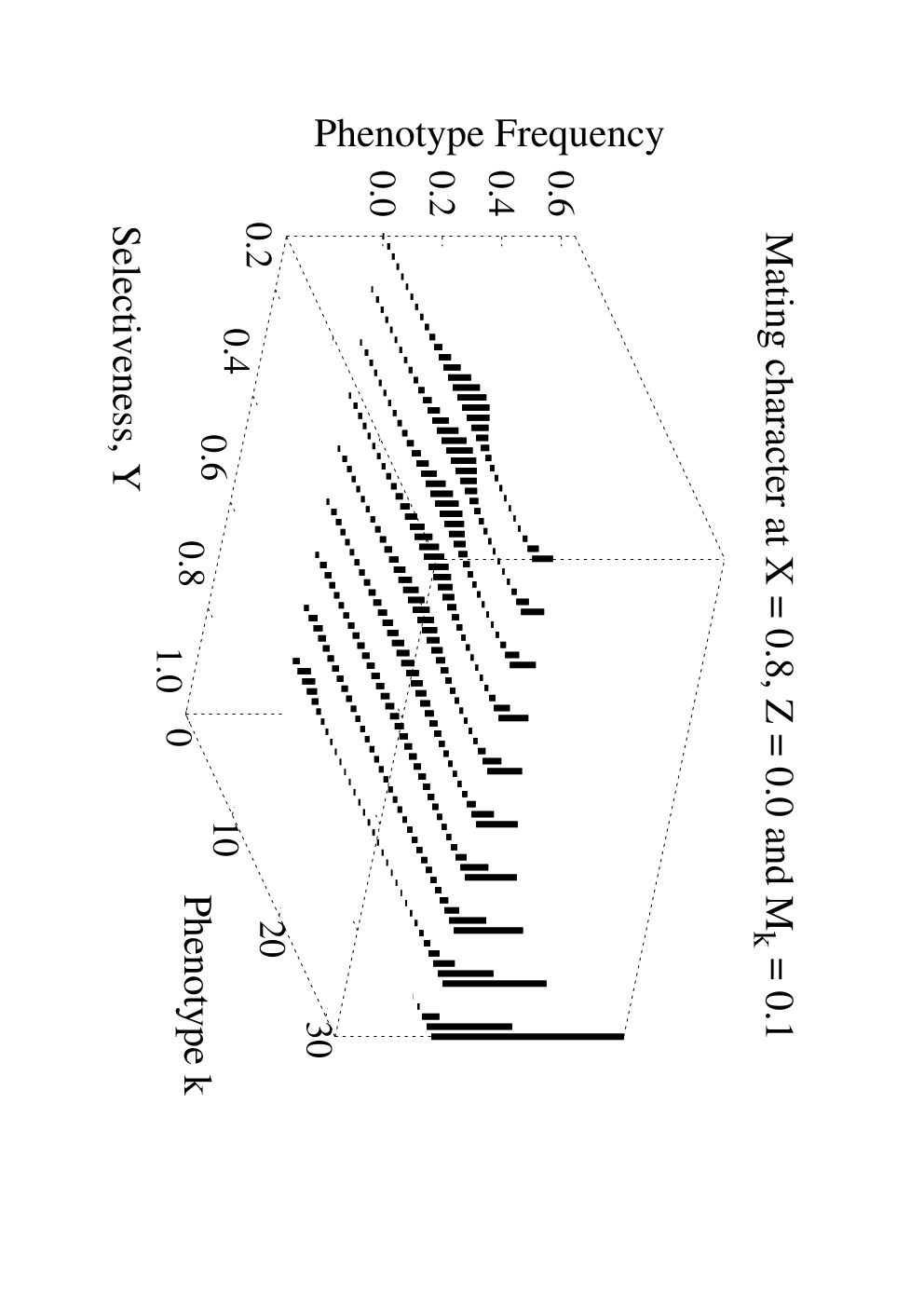
In what follows, the character determining sexual selection in the population is the colour of the individuals and the character that determines natural selection is the individuals’ jaws morphology, which is the case in the Midas cichlid species complex. In common with A. Labiatus species, Fig.1, it is possible to find polychromatism and monomorphism in the ecological character for all values of the asymmetrical competition strength between the intermediate and specialist phenotypes smaller than one, in Eq. (3) and (2), provided the following conditions are met: (i) no disruptive natural selection , (ii) a sexual selection strength in the population, and (iii) a large value for the mutation probability of the mating character , Fig. 2 (b).
III.2 Simulations for A. Zaliosus species
The characteristics of the A. Zaliosus species is to have a unimodal distribution for the mating trait and a bimodal distribution for the ecological one. We have already seen, in the previous section, that for there is no splitting of the ecological trait, unless if and . On the other side, for and the mating trait is also splitted, which is not the case of A. Zaliosus species. So in order to simulate the A. Zaliosus process of speciation, we will take and will first study each trait separately.


Fig. 4 (a) shows the distribution of the ecological trait for and . From this figure we see that this distribution changes from a unimodal one to a bimodal distribution depending on the value of the disruptive natural selection strength, . For , the existing intermediate phenotypes belong to individuals that die before reaching the minimum reproductive age. Fig. 4 (b) shows the distribution of the mating trait, also for and . It can be seen that the distribution is unimodal only for ; for it is almost bimodal but not completely, since the intermediate population, , is appreciable. The existence of the intermediate phenotypes is due to the panmictic behaviour of the population,
The phenotype frequency of the ecological trait, Fig. 4 (a), does not change if we vary the mutation probabilities and . The phenotype frequency of the mating trait also does not change for . The same is not true when , since then the distribution is trimodal, Fig. 5, with peaks at , and when .

From these results we may conclude that when , the splitting of the mating trait is favoured by small mutation probabilities, , of this trait, which is not what we want for the A. Zaliosus species. From Figs. 4 (a) and (b) we can see that the proper regions of parameters to simulate the speciation process of this species are , bimodal distribution for the ecological trait, and , unimodal one for the mating trait.
III.3 Simulations for A. Citrinellus species
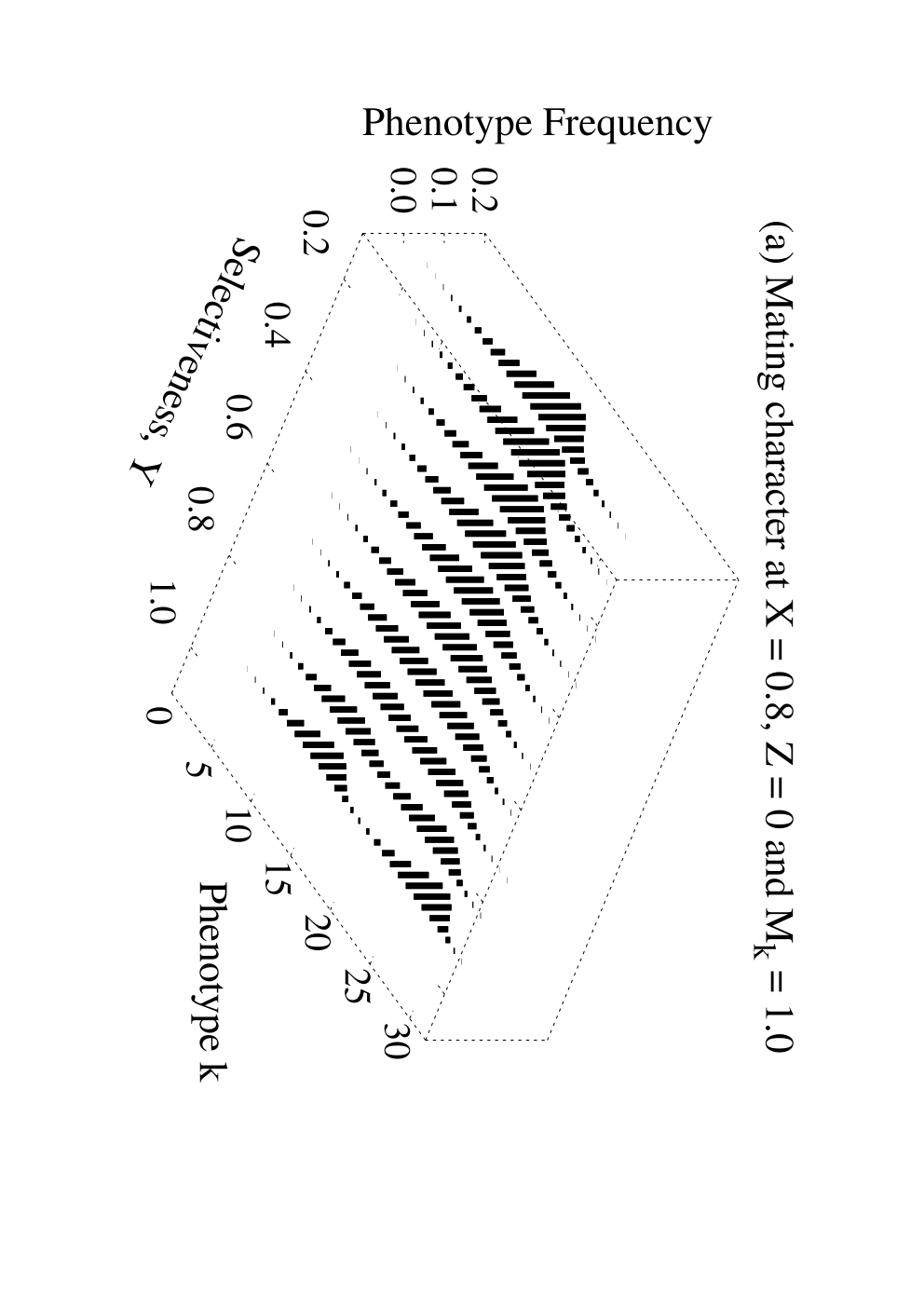
One way to obtain the polycromatism and polymorphism characteristic of the A. Citrinellus species, bimodal distributions of the both traits, is to consider uniform distribution of resources without disruptive natural selection. We have already shown that simulations with and , only assortative mating, give a bimodal distribution for the mating trait, Fig. 2 (b), independently of the competition strength, , provided the mutation probability is . However, to obtain also bimodal distribution of the ecological trait, without disruptive natural selection, it is necessary to have , that is, a symmetric competition between specialist and intermediate phenotypes, as shown in Fig. 6.
For , it is also possible to split both phenotype distributions, but then it is necessary to consider small mutation probabilities of the mating trait, , a weak assortative mating, , and proper values of the resource distribution, , depending on the competition strength, . For instance, for , Fig 4 (a).

IV Discussion
Although competition for resources and natural disruptive selection appear together in Eq. (2) and (3), they lead to rather different situations. While competition depends on the population sizes and affects equally individuals of the same phenotypic group, disruptive natural selection caused by resources distributions acts on each particular individual, according to its phenotype. As a result, disruptive selection becomes more effective than competition. For instance, even for a panmictic behaviour, disruptive natural selection may lead to a splitting of both traits, depending only on the values of and , as already pointed in dd. A small mutation probability of the mating trait also favours this double splitting, as obtained in kk.
On the other hand, in order to split both phenotypic distributions without disruptive natural selection, , it is imperative to have sexual selection, and now the splitting process depends on the values of and , and in this case the mutation of the mating trait must be large in order to prevent genetic drift effects.
Anyway, the A. Citrinellus case is the evolution of the splitting in both traits distributions must be driven by disruptive natural selection or by sexual selection, and the only statistical difference we found between these two scenarios is that the correlation between the traits is smaller when the splitting is driven by sexual selection. It so happens because the large mutation rate of the mating trait, mentioned above, introduces large fluctuations in this correlation.
Acknowledgements.
We thank the agencies CNPq, FAPERJ (E-26/170.699/2004), and CAPES for financial support and J. Nogales for fruitful discussions.References
- (1) Mayr E., 1963, Animal Species and Evolution, Belknap Press.
- (2) Bush G. L., 1969, Evolution, 23, 237-251.
- (3) Douglas J. Futuyma, 1979, Evolutionary biology (2nd edn), Sinauer.
- (4) Marta Barluenga, Kai N. Stolting, Walter Salzburger, Moritz Muschick and Axel Meyer, 2006, Sympatric speciation in Nicaraguan crater lake cichlid fish, Nature, 439, 719-723.
- (5) U. K. Schliewen, T. D. Kocker, K. R. McKaye, O Seehausen and D. Tautz, 2006, Evolutionary Biology: Evidence for sympatric speciation?, Nature, 444, E12-E13.
- (6) Barlow G. W. and Munsey J. W. (1976), The red devil-Midas-arrow cichlid species complex in Nicaragua. In: Investigations of the Ichthyofauna of Nicaraguan Lakes (ed. Thorson TB), pp.359-369. University of Nebraska Press, Lincoln, NB.
- (7) Marta Barluenga and Axel Meyer (2004), The Midas cichlid species complex: incipient sympatric speciation in Nicaraguan cichlid fishes, Molecular Ecology, 13, 2061-2076.
- (8) Anthony B. Wilson, Katharina Noack-Kunnmann and Axel Meyer 2000, Incipient speciation in sympatric Nicaraguan crater lake cichlid fishes: sexual selection versus ecological diversification, Proc. R. Soc. Lond. B, 267, 2133-2141.
- (9) Axel Meyer (1989), Cost of morphological specialization: feeding performance of the two morphs in the trophically polymorphic cichlid fish, Cichlasoma citrinellum. Oecologia, 80, 431-436.
- (10) Sara Via, Review, TRENDS in Ecology Evolution, Sympatric speciation in animals: the ugly duckling grows up, 16(7), 381-390 (2001).
- (11) Alexey S. Kondrashov and Fyodor A. Kondrashov (1999), Interactions among quantitative traits in the course of sympatric speciation, Nature, 400, 351-354.
- (12) Ulf Dieckmann and Michael Doebeli (1999), On the origin of species by sympatric speciation, Nature, 400, 354-357.
- (13) M. Higashi, G. Takimoto N. Yamamura (1999), Sympatric Speciation by sexual selection, Nature, 402, 523-526.
- (14) Gavrilets S. (2000), Rapid evolution of reproductive barriers driven by sexual conflict, Nature, 403, 886-889.
- (15) K. Luz-Burgoa, Tony Dell and S. Moss de Oliveira, Computer simulations for sympatric speciation in a simple food web, Phys. Rev. E, 72, 011914 (2005).
- (16) K. Luz-Burgoa, S. Moss de Oliveira, Veit Schwämmle and J. S. Sá Martins, Thermodynamic behavior of a phase transition in a model for sympatric speciation, Phys. Rev. E, 74, 021910 (2006).
- (17) T.J.P. Penna, J. Stat. Phys. 78, 1629 (1995).