Reliability of Coupled Oscillators II:
Larger Networks

We consider in this paper networks of coupled phase oscillators in the presence of external stimuli. A schematic picture of such a setup is shown in Figure 1. The networks considered are of the type that arise in many settings; see e.g., [30, 34, 19, 14, 42, 32, 3, 5, 7].

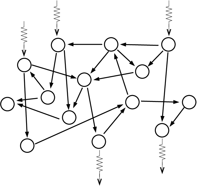
The unforced systems, i.e., the systems without external stimuli, are described by

In this paper, $N$ can be any number $\geq 1$; in particular, it can be arbitrarily large. The state of oscillator $i$ is described by an angular variable $\theta_{i}\in S^{1}\equiv{\mathbb{R}}/{\mathbb{Z}},i=1,\cdots,N$. Its intrinsic frequency is given by a constant $\omega_{i}$. We allow these frequencies to vary from oscillator to oscillator. The second term on the right represents the coupling: $a_{ji}\in{\mathbb{R}}$, $g$ is a “bump function” vanishing outside of a small interval $(-b,b)$; on $(-b,b)$, it is smooth, $\geq 0$, and satisfies $\int_{-b}^{b}{g(\theta)\ d\theta}=1$; $z(\theta)$ is a function which in this paper is taken to be $z(\theta)=\frac{1}{2\pi}(1-\cos(2\pi\theta))$. The meaning of this coupling term is as follows: We say the $j$th oscillator “spikes” when $\theta_{j}(t)=0$. Around the time that an oscillator spikes, it emits a pulse which modifies some of the other oscillators [29, 35, 13, 27]. The sign and magnitude of $a_{ji}$ describe how oscillator $j$ affects oscillator $i$: $a_{ji}>0$ (resp. $a_{ji}<0$) means oscillator $j$ excites (resp. inhibits) oscillator $i$ when it spikes, and $a_{ji}=0$ means oscillator $i$ is not directly affected. In this paper, $b$ is taken to be about $\frac{1}{20}$, and the $a_{ji}$ are taken to be ${\mathcal{O}}(1)$. Finally, the function $z(\theta)$, often called the phase response curve [41, 11, 6, 19], measures the variable sensitivity of an oscillator to coupling and stimulus inputs.

The stimulus-driven systems are of the form

Here, $I_{i}(t)$ is the external stimulus received by oscillator $i$; it is taken to be white noise with amplitude $\epsilon_{i}$. For simplicity, we assume that for $i\neq j$, $dW_{i}(t)$ and $dW_{j}(t)$ are either independent, or they are one and the same, i.e., the same input is received by both oscillators although the amplitudes may differ. As discussed earlier, we are primarily interested in situations where inputs are received by only a subset of the oscillators, with $\epsilon_{i}\approx 0$ for the rest. Likewise, we are sometimes interested in the response registered at only a subset of the oscillators rather than the whole network. See Fig. 1.

For more on the motivation and interpretation of this model, see Sect. 1.2 of  [21].

Reliability in this paper refers to the following: Suppose the stimuli in Eq. (2) described by the terms $\varepsilon_{i}I_{i}(t)$ are turned on at time $t=0$. Will the response of the system depend on the initial state of the system when the stimuli are presented? That is to say, let ${\bf\Theta}(t)$ be the solution of Eq. (2). To what degree does ${\bf\Theta}(t)$ depend on ${\bf\Theta}(0)$ after some initial period of adjustment? If the dependence on ${\bf\Theta}(0)$ is negligible after a transient, we think of the system is reliable; and if different ${\bf\Theta}(0)$ lead to persistently different responses at time $t$ for all or most $t$, we say the system is unreliable. Needless to say, the lengths of the transient and the degree to which the responses differ are important in practical situations, but these issues will not be considered here.

The measure of reliability used in a good part of this paper is $\lambda_{\rm max}$, the largest Lyapunov exponent of the system. We briefly recall here the meaning of this number and its relation to reliability as discussed above, referring the reader to [1, 2] for background material on stochastic flows and to Sect. 2 of [21] for a more detailed discussion of how this material is used in the study of reliability.

We view Eq. (2) as a stochastic differential equation (SDE) on ${\mathbb{T}}^{N}\equiv S^{1}\times\cdots S^{1}$ with phase variables $(\theta_{1},\cdots,\theta_{N})$. A well known theorem gives the existence of a stochastic flow of diffeomorphisms. That is to say, for almost every realization $\omega$ of white noise, there exist flow maps of the form $F_{t_{1},t_{2};\omega}$: here $t_{1}<t_{2}$ are any two points in time, and $F_{t_{1},t_{2};\omega}({\bf\Theta}(t_{1},\omega))={\bf\Theta}(t_{2},\omega)$ where ${\bf\Theta}(t,\omega)$ is the solution of (2) corresponding to $\omega$. By the Lyapunov exponents of Eq. (2), we refer to the Lyapunov exponents of $F_{0,t;\omega}$ as $t$ increases. These numbers do not depend on $\omega$; and they do not depend on ${\bf\Theta}(0)$ if Eq. (2) is ergodic (which it often is). The largest Lyapunov exponent is denoted by $\lambda_{\rm max}$.

In  [21], cf. [33, 9, 17], we used of $\lambda_{\rm max}$ as a measure of reliability. Specifically, $\lambda_{\rm max}<0$ is equated with reliability, $\lambda_{\rm max}>0$ represents unreliable behavior, and $\lambda_{\rm max}=0$ is inconclusive.¹¹ 1 We note that there are other ways to measure unreliability which seem to us to be equally reasonable. For example, one can take the sum of all positive Lyapunov exponents. These criteria will continue to be used in this paper.

To understand why $\lambda_{\rm max}$ is a reasonable indicator of reliability, recall the idea of sample measures: if we let $\mu$ denote the stationary measure of (2), i.e. the stationary solution to the Fokker-Planck equation, the sample measures are then the conditional measures of $\mu$ given the past history of the stimuli. More precisely, if we think of $\omega$ as defined for all $t\in(-\infty,\infty)$ and not just for $t>0$, then $\mu_{\omega}$ describes what one sees at $t=0$ given that the system has experienced the input defined by $\omega$ for all $t<0$. Sample measures thus give an approximation of what one sees in response to an input presented on a time interval $[-t_{0},0)$ for large enough $t_{0}>0$. If we let $\sigma_{t}$ denote the time-shift of the Brownian path $\omega$, then sample measures evolve in time according to $(F_{0,t;\omega})_{*}\mu_{\omega}=\mu_{\sigma_{t}\omega}$. As explained in  [21], if stimuli corresponding to a realization $\omega$ are turned on at $t=0$, then $\mu_{\sigma_{t}\omega}$ gives a good approximation of the responses of the system at sufficiently large times $t$ for an ensemble of initial conditions sampled from a smooth density. In particular, if $\mu_{\sigma_{t}\omega}$ collapses down to a single point as $t$ increases, then we conclude that initial conditions have little effect after transients, i.e. the system is reliable. If $\mu_{\sigma_{t}\omega}$ is spread out nontrivially in the phase space, and this condition persists with $t$, then we conclude that different initial conditions have led to different responses at time $t$, which is exactly what it means for the system to be unreliable.

The relation between sample measures, which represent a collection of the system’s possible responses, and $\lambda_{\rm max}$, its top Lyapunov exponent, is summarized in the following general result from dynamical systems theory.

Case (1) is often referred to as the system having random sinks. When $\lambda_{\rm max}<0$, in the vast majority of situations $\mu_{\omega}$ is supported on a single point; we therefore equate it with reliability as in, e.g., [33, 28]. In Case (2), the system is said to have a random strange attractor. For deterministic systems, SRB measures are well studied objects with a distinctive geometry: they have densities on (typically) lower dimensional surfaces that wind around the phase space in a complicated way; see [4]. Here we have a random (i.e. $\omega$-dependent) version of the same picture. Thus the resulting geometry is a readily recognizable signature of unreliability.

Finally, we remark that $\lambda_{\rm max}$ is a global indicator of unreliability, meaning a positive exponent will tell us only that the network possesses some unreliable degrees of freedom: it does not specify where this unreliability is produced, whether its effects are localized, and so on. Different measurements are needed to answer these more refined questions. They are discussed in Sects. 3–6.

This section discusses an issue that did not arise in  [21]. Our criterion for unreliability, $\lambda_{\rm max}>0$, is generally equated with chaos. In the 2-oscillator network studied in [21], this chaotic behavior is triggered by the input: without this forcing term, the system cannot be chaotic as it is a flow on a two-dimensional surface. The situation is quite different for larger networks.

We begin by explaining what we mean by “chaotic.” It is well known that systems of 3 or more coupled oscillators without external input can have complicated orbits, such as homoclinic orbits or horseshoes (see, e.g., [31, 27], and also [12, 5] for general references). These special orbits by themselves do not necessarily constitute a seriously chaotic environment, however, for they are not always easily detectable, and when horseshoes coexist with sinks, the chaotic behavior seen is transient for most choices of initial conditions. We claim here that networks with 3 or more oscillators can support a stronger form of chaos, namely that of strange attractors. There is no formal definition of the term “strange attractors” in rigorous dynamical systems theory. An often used characterization is the existence of SRB measures or physical measures, which describe the long-time distribution of orbits starting from positive Lebesgue measure sets of initial conditions [4, 43, 44]. At a minimum, one would insist that positive Lyapunov exponents be observed for almost all – or at least on a large positive Lebesgue measure set – of initial conditions. (In the case of horseshoes coexisting with sinks, for example, Lyapunov exponents for most initial conditions are negative after a transient.) In numerical simulations, one has to settle for positive Lyapunov exponents that are sustained over time for as many randomly chosen initial conditions as possible. This will be our operational definition of intrinsic network chaos.

One of the simplest configurations that support intrinsic network chaos is

(3)

The setup above is similar to that studied in [21], except that the (2,3)-subsystem is kicked periodically by pulses from oscillator 1 rather than driven by an external stimulus in the form of white noise. Ignoring the presence of oscillator 1 for the moment, we saw in [21], Sect. 4.2, that when $a_{23}$ and $a_{32}$ are roughly comparable and away from $0$, the phase space geometry of oscillators 2 and 3 is favorable for shear-induced chaos, a geometric mechanism for producing chaotic behavior. Indeed, a rigorous theory of this mechanism gives the existence of strange attractors with SRB measures when such a system is periodically kicked — provided the kicks are suitably directed and time intervals between kicks are sufficiently large [39, 40]. Even though the kick intervals (of $\approx 1$) here are too short for rigorous results to be applicable, numerical simulations show that there are definitively positive exponents sustained over long periods of time when $a_{12}$ is large enough.

As an example, consider system (3) with $\omega_{1},\omega_{2},\omega_{3}=0.93,1,1.1$, and $a_{23},a_{32}=1,1.45$. We find that $\lambda_{\rm max}$ increases from about $0.025$ to $0.12$ for $a_{12}\in(1,1.5)$.²² 2 These Lyapunov exponents are computed starting from $\sim 10$ initial conditions and have an absolute error of roughly 0.005. Notice that the system parameters above are chosen so that the (2,3)-subsystem is unreliable, that is, so that $\lambda_{\rm max}>0$ when oscillator 2 receives a white noise stimulus: see [21], Fig. 12. It is, after all, the same mechanism, namely shear-induced chaos, that produces the chaos in both situations. See [22], Study 4, for similar findings.

While there are certainly large classes of networks that do not exhibit intrinsic network chaos (e.g. see Sect. 3), from the example above one would expect that such chaos is commonplace among larger networks. Moreover, for intrinsically chaotic networks, one would expect $\lambda_{\rm max}$ to remain positive when relatively weak stimuli are added to various nodes in the network. We have, in fact, come across a number of examples in which $\lambda_{\rm max}$ remains positive for larger stimulus amplitudes. This raises the following issue of interpretation: In an intrinsically chaotic network that also displays $\lambda_{\rm max}>0$ in the presence of inputs, it is unclear how to attribute the source of unreliability, since the effects of inputs and intrinsic chaos are largely inseparable. We adopt here the view that whatever the cause, such a network is unreliable.

An interesting question is whether or not networks with intrinsic chaos of the form described above, i.e. with $\lambda_{\rm max}>0$ for large sets of initial conditions in the absence of inputs, necessarily respond unreliably to external stimuli. We find that the answer is “no”: we have come across a number of instances where weakly chaotic networks are stabilized by sufficiently strong inputs. An example is in the following 3-cell ring:

(4)

The phase space of system (4) is the $3$-torus. Taking the section $\{\theta_{1}=0\}$ of the $\varepsilon=0$ flow, we obtain a return map $\Psi$ from the $2$-torus to itself. There are well known examples of maps of the $2$-torus that are uniformly hyperbolic; a case in point is the “cat map”. These maps are robustly hyperbolic; it is impossible to destroy their positive Lyapunov exponents by reasonable-size perturbations. Our section map $\Psi$, however, cannot be of this type for topological reasons: it is not hard to see that $\Psi$ can be deformed continuously to the identity map by suitably tuning system parameters. Generally speaking, for $2$-D maps that can be deformed to the identity, the only way to form strange attractors is by “folding”. Such systems are at best nonuniformly hyperbolic; their observed Lyapunov exponents are the results of competing tendencies: there is expansion in the phase space, which necessarily leads to contraction elsewhere or in different directions, and the expanding and contracting directions are not separated as in the cat map. As a result of this competition, sustained, observable chaos, i.e., strange attractors, live side by side in parameter space with transient chaos, i.e., systems in which horseshoes and sinks coexist. The simplest family of examples exhibiting such a phenomenon is the logistic family [23, 15, 10]. This phenomenon also occurs in shear-induced chaos; see e.g., [22]. For an exposition on nonuniformly hyperbolic systems, see e.g., [43]. The mixed behavior alluded to above is discussed in, e.g. [44].

Thus even without explicit knowledge of the map $\Psi$, one would expect to see a pattern of behavior similar to that in Fig. 2(a) when positive exponents are present. Here, $\lambda_{\rm max}=0$ for the flow corresponds to $\Psi$ having a Lyapunov exponent $\leq 0$, including the parameters with transient chaos.

We now consider the effects of adding a stimulus, that is, taking $\varepsilon>0$ for system (4). Informally, one may think of the stimulus as sampling nearby parameters, averaging (in a loose sense) the different tendencies, with chaos suppression made possible by the presence of the mixed behavior. A sample of our numerical results is shown in Fig. 2(b). At $\varepsilon=0$, $\lambda_{\rm max}>0$, indicating network chaos. As expected, $\lambda_{\rm max}$ remains positive for small $\varepsilon$. But, as $\varepsilon$ increases, $\lambda_{\rm max}$ steadily decreases and eventually becomes mildly negative, demonstrating that sufficiently strong forcing can suppress intrinsic network chaos and make a network more reliable. A possible mechanistic explanation is that when $\varepsilon$ is large enough, oscillator 1 is affected more by the stimulus than by oscillator 3 due to the relatively weak coupling $a_{31}$. As in the case of a single oscillator, the stimulus has a stabilizing effect on oscillator 1, making it reliable.

Our understanding from the discussion above may be summarized as follows:

We first describe the connection graph that corresponds to an oscillator network. Let each node of this graph, $i\in\{1,\cdots,N\}$, correspond to an oscillator. Assign a directed edge from node $i$ to node $j$, $i\neq j$, if oscillator $i$ provides input to oscillator $j$, i.e. if $a_{ij}\neq 0$; in this case, we write $i\to j$. (For simplicity, we do not allow nodes to connect to themselves.) A cycle in such a directed graph is a sequence of nodes and edges $i_{1}\to i_{2}\to\cdots i_{k}\to i_{1}$ for some $k>1$.

Given any pair of oscillators in an acyclic network, either they are “unrelated”, or one is “upstream” from the other. We say oscillator $i$ is “upstream” from oscillator $j$ if there is a sequence of nodes and edges that goes from $i$ to $j$. The absence of cycles is precisely what makes this “upstream”–“downstream” notion well defined. We say oscillators $i$ and $j$ are “unrelated” if there is no chain that goes from $i$ to $j$ or vice versa. Unrelated oscillators do not necessarily behave independently: they may, for example, receive input from the same source. Overall, the structures of acyclic networks can still be quite complex, with tree-like branching and recombinations possible.

Our first task is to find a systematic way to treat the dynamics within these networks.

Using the notation of Sect. 1.1, we now discuss the dynamical structure of acyclic oscillator networks. First, let $\varphi_{t}$ denote the flow on ${\mathbb{T}}^{N}$ in the absence of inputs, i.e., with $\varepsilon_{i}\equiv 0$. We say $\varphi_{t}$ factors into a hierarchy of skew-products with 1-dimensional fibers if after a permutation of the names of the $N$ oscillators, we have the following: For each $k=1,\cdots,N$, there is a vector field $X^{(k)}$ on ${\mathbb{T}}^{k}$ such that if $\varphi_{t}^{(k)}$ is the flow generated by $X^{(k)}$, then (i) $\varphi_{t}^{(k)}$ describes the dynamics of the network defined by the first $k$ oscillators and the relations among them, and (ii) $\varphi^{(k+1)}_{t}$ is a skew-product over $\varphi^{(k)}_{t}$, that is, the vector field $X^{(k+1)}$ on ${\mathbb{T}}^{k+1}$ has the form

where $\{Y_{(\theta_{1},\cdots,\theta_{k})}\}$ is a family of vector fields on $S^{1}$ parametrized by $(\theta_{1},\cdots,\theta_{k})\in{\mathbb{T}}^{k}$. In particular, $\varphi^{(N)}_{t}=\varphi_{t}$. In the system defined by (5), we refer to $\varphi_{t}^{(k)}$ on ${\mathbb{T}}^{k}$ as the flow on the base, and each copy of $S^{1}$ over ${\mathbb{T}}^{k}$ as a fiber.

Next we generalize to acyclic networks with stimuli. Such networks can also be represented by a directed graph of the type described above, except that some of the nodes correspond to stimuli and others to oscillators. If $i$ is a stimulus and $j$ an oscillator, then $i\to j$ if oscillator $j$ receives information directly from stimulus $i$. No arrow can terminate at a stimulus, so that $m(i)=0$ if $i$ is a stimulus. Clearly, a network driven by stimuli is acyclic if and only if the corresponding network without stimuli is acyclic.

Proceeding to skew-product representations, consider first the case of a single oscillator driven by a single stimulus. Let $\Omega$ denote the set of all Brownian paths defined on $[0,\infty)$, and let $\sigma_{t}:\Omega\to\Omega$ be the time shift. Then the dynamics of the stochastic flow discussed in Sect. 2.1 can be represented as the skew-product on $\Omega\times S^{1}$ with

Similarly, a network of $N$ oscillators driven by $q$ independent stimuli can be represented as a skew-product with base $\Omega^{q}$ (equipped with product measure) and fibers ${\mathbb{T}}^{N}$.

Consider a network of $N$ oscillators driven by $q$ independent stimuli. We first review some notation. Let $\omega\in\Omega^{q}$ denote a $q$-tuple of Brownian paths, and let $F_{0,t;\omega}$ denote the corresponding stochastic flow on ${\mathbb{T}}^{N}$. For a fixed $\omega\in\Omega^{q},x\in{\mathbb{T}}^{N}$ and tangent vector $v$ at $x$, define the Lyapunov exponent

if this limit exists. If $\mu$ is a stationary measure of the stochastic flow, then for a.e. $\omega$ and $\mu$-a.e. $x$, $\lambda_{\omega}(x,v)$ is well defined for all $v$. The following is the main result of this section:

Before proceeding to a proof, it is useful to recall the following facts about Lyapunov exponents. For a.e. $\omega$ and $\mu$-a.e. $x$, there is an increasing sequence of subspaces $\{0\}=V_{0}\subset V_{1}\subset\cdots\subset V_{r}={\mathbb{R}}^{N}$ and numbers $\lambda_{1}<\cdots<\lambda_{r}$ such that $\lambda_{\omega}(x,v)=\lambda_{i}$ for every $v\in V_{i}\setminus V_{i-1}$. The subspaces depend on $\omega$ and $x$, but the exponents $\lambda_{j}$ are constant a.e. if the flow is ergodic. We call a collection of $N$ vectors $\{v_{j}\}$ a Lyapunov basis if exactly $\dim(V_{i})-\dim(V_{i-1})$ of these vectors are in $V_{i}\setminus V_{i-1}$. If $\{v_{j}\}$ is a Lyapunov basis, then for any $u,v\in\{v_{j}\}$, $u\neq v$,

that is, angles between vectors in a Lyapunov basis do not decrease exponentially fast; see e.g.,  [43] for a more detailed exposition.

For $k=1$, $\lambda_{\omega}(x,v)\leq 0$ for a.e. $\omega$ and $\mu^{(1)}$-a.e. $x$. This is a consequence of Jensen’s Inequality; see e.g., [21], Sect. 2.2, for more detail.

Assume we have shown the conclusion of Theorem 2 up to $k-1$, and view $F^{(k)}_{0,t;\omega}$ as a skew-product over $\Omega^{q}\times{\mathbb{T}}^{k-1}$ with $S^{1}$-fibers. Choose a vector $v_{k}$ in the direction of the $S^{1}$-fiber. Note that this direction is invariant under the variational flow $DF^{(k)}_{0,t;\omega}$ due to the skew-product structure. Starting with $v_{k}$, we complete a Lyapunov basis $\{v_{1},\cdots,v_{k}\}$ at all typical points. Due to the invariance of the direction of $v_{k}$, we may once more use Jensen’s Inequality to show that $\lambda_{\omega}(x,v_{k})\leq 0$ for a.e. $x$ and $\omega$. We next consider $v_{i}$ with $i<k$. First, define the projection $\pi:{\mathbb{T}}^{k}\to{\mathbb{T}}^{k-1}$, and note that

Due to Eq. (7), we have $\lambda_{\omega}(x,v_{i})=\lim_{t\rightarrow\infty}\frac{1}{t}\log|\pi(DF^{(k)}_{0,t;\omega}(x)v_{i})|$. But the skew-product structure yields $\pi(DF^{(k)}_{0,t;\omega}(x)v_{i})=DF^{(k-1)}_{0,t;\omega}(\pi x)(\pi v_{i})$, so by our induction hypothesis, $\lambda_{\omega}(x,v_{i})\leq 0$. $\square$

Arguments similar to those in the proof of Theorem 2 (but in the absence of stimuli and without the use of an invariant measure) give the following:

We next describe how the reliability of more general networks may be analyzed by decomposition into subunits. Consider a graph with nodes $\{1,\cdots,N\}$ as in the beginning of Sect. 3.1, and let $\sim$ be an equivalence relation on the set $\{1,\cdots,N\}$. The quotient graph defined by $\sim$ has as its nodes the equivalence classes $[i]$ of $\sim$, and we write $[i]\to[j]$ if there exists $i^{\prime}\in[i]$ and $j^{\prime}\in[j]$ such that $i^{\prime}\to j^{\prime}$. The following is a straightforward generalization of Proposition 3.2:

We pause to discuss in more detail the structure in Prop 3.4, as it is important in the rest of this paper. An equivalence relation on the nodes of a network describes a decomposition of the network into smaller subunits called modules. Introducing directed edges between modules as above, we obtain what we call a quotient network in this paper. Assume this quotient network is acyclic, and let $M_{1},M_{2},\cdots,M_{p}$ be the names of the modules ordered in such a way that $M_{i}$ is upstream from or unrelated to $M_{j}$ for all $j>i$. Let $k_{j}$ be the number of nodes in module $M_{j}$. For $s_{i}=k_{1}+k_{2}+\cdots+k_{i}$, let $F^{(s_{i})}_{0,t,\omega}$ denote, as before, the stochastic flow describing the dynamics within the union of the first $i$ modules; we do not consider $F^{(s)}_{0,t,\omega}$ when $s\neq s_{i}$ for some $i$. The dynamics of the entire network can then be built up layer by layer as follows: We begin with the stochastic flow $F^{(k_{1})}_{0,t,\omega}$. Then proceed to $F^{(k_{1}+k_{2})}_{0,t,\omega}$, which we view as a skew-product over $F^{(k_{1})}_{0,t,\omega}$. This is followed by $F^{(k_{1}+k_{2}+k_{3})}_{0,t,\omega}$, which we view as a skew-product over $F^{(k_{1}+k_{2})}_{0,t,\omega}$, and so on.

Let $\lambda^{(1)}_{1},\cdots,\lambda^{(1)}_{k_{1}}$ denote the Lyapunov exponents of $F^{(k_{1})}_{0,t,\omega}$. Clearly, these are the Lyapunov exponents of a network that consists solely of module $M_{1}$ and the stimuli that feed into it. We wish, however, to view $M_{1}$ as part of the larger network. If $\lambda^{(1)}_{\max}\equiv\max_{j}\lambda^{(1)}_{j}>0$, we say unreliability is produced within $M_{1}$. An interesting question is the effect of this unreliability on sites downstream. Leaving this to Sect. 4, we continue with the present discussion: For $i>1$, let $\lambda^{(i)}_{1},\cdots,\lambda^{(i)}_{k_{i}}$ denote the fiber Lyapunov exponents in the skew-product representation of $F^{(s_{i})}_{0,t,\omega}$ over $F^{(s_{i-1})}_{0,t,\omega}$, and let $\lambda^{(i)}_{\max}=\max_{j}\lambda^{(i)}_{j}$. Then $\lambda^{(i)}_{\max}>0$ has the interpretation that unreliability is produced within module $M_{i}$ as it operates in the larger network. It is important not to confuse this with the Lyapunov exponents of module $M_{i}$ in isolation, an issue we will follow up in Sect. 6.

Analogous interpretations for the zero-input systems are obvious: for $i>1$, $\lambda^{(i)}_{\max}>0$ at $\varepsilon=0$ means there is intrinsic network chaos within the module $M_{i}$ as a subsystem of the larger system, and so on.

The proof of the following result is virtually identical to that of Theorem 2:

As noted earlier, the idea of “upstream”–“downstream” for acyclic networks extends to modules connected by acyclic graphs, so that it makes sense to speak of a module as being downstream from another module, or a site as being downstream from another site, meaning the modules in which they reside are so related.

Often, it is the response of a network measured at specific oscillators (or sites) that is of relevance, rather than the response of the network as a whole. While $\lambda_{\rm max}>0$ tells us that there is unreliability somewhere in the system, it does not tell us which oscillators are affected. To capture the idea of reliability at individual sites, recall that the reliability of the entire system is reflected in the sample measures $\mu_{\omega}$ (see Sect. 1.2). By the same reasoning, the reliability at site $i$ is reflected in the marginals of $\mu_{\omega}$ in the variable $\theta_{i}$; we denote this marginal distribution by $\mu_{\omega,i}$. We say a network is reliable at site $i$ if $\mu_{\omega,i}$ is concentrated at a single point; the more uniformly distributed these projected sample measures are, the greater the site unreliability. These ideas are easily generalized to groups of more than one site, but we will treat only single site reliability.

The following are three standard ways in which the distribution of $\mu_{\omega,i}$ can be described:

Above, we discussed various ways to assess $\mu_{\omega,i}$ from a purely theoretical standpoint. Returning to the situation at hand, recall from Theorem 1 that when $\lambda_{\rm max}>0$, i.e. when the system is unreliable, $\mu_{\omega}$ is a random SRB measure. These measures have densities on complicated families of smooth manifolds. In particular, they have dimensions $>1$; e.g. in the case of 2 oscillators, the dimension of the random SRB measures is $1+\alpha$ for some $\alpha\in(0,1)$ where $\alpha$ describes the dimension of the fractal part. A well known result in analysis [24] tells us that when measures of dimensions $>1$ are projected onto 1-dimensional subspaces, the projected measures have a density for projections along almost all directions. Now not all projections are “good” in this sense, and we cannot be certain that the projection onto any particular site is “good” (projections onto sites upstream from where unreliability is produced are obviously not). Still, if the projection to site $i$ is good, then $\lambda_{\rm max}>0$ would imply that $\mu_{\omega,i}$ has a density. This being the case, it is more important to be able to compare different distributions with densities than to distinguish different singular distributions. We therefore favor site entropy over information dimension as a measure of site reliability.

In this paper, we will use a combination of site entropy and CDFs: If the computed values of $H(i)$ appear bounded below, then it is safe to conclude site unreliability, and the closer $H(i)$ is to $0$, the more unreliable. If, on the other hand, the computed values of $H(i)$ appear unbounded, then CDFs are used to confirm site reliability.

We now return to the question of propagation of unreliability to sites downstream from an unreliable module. The simplest network with which to investigate this is the $N$-chain system

(8)

Suppose we choose $a_{12}$, $a_{21}$, and $\varepsilon_{1}$ so that the (1,2)-subsystem is unreliable. Notice that no unreliability is produced elsewhere. The question is: will this unreliability be observable downstream, at sites $i=3,4,\cdots,N$, or does it somehow “dissipate?” We run the following numerical experiment: we set $\omega_{1}=1$, $\omega_{2}=1.05$, $a_{12}=1$, $a_{21}=1.05$, and $\varepsilon_{1}=1$, so that the Lyapunov exponent $\lambda_{\rm max}$ of the (1,2)-subsystem is $\approx 0.1$. For $i\geq 3$, we draw randomly (and fix) $\omega_{i}$ from $[0.9,1.1]$ and $a_{i,i+1}$ from $\pm[0.6,1.2]$. Computing the site entropies³³ 3 We compute site entropies by simulating the response of $10,000$ initial conditions to the same realization of the stimulus, then applying the “binless” estimator of Kozachenko and Leonenko [18] (see also [38]). ${H}(i)$ for sites $i=3,7,10$, we find:

To help interpret these numbers, recall that identifying $S^{1}$ with $[0,1]$, the entropy of the uniform distribution on an interval $[a,b]$ is $\log(b-a)$, and $\log\frac{1}{2}\approx-0.7$. The data above thus indicate that the site distributions are fairly uniform, and in fact seem to become more uniform for sites farther downstream. Fig. 3 shows the corresponding CDFs for some sites at representative times; CDFs at other sites are qualitatively similar. The graphs clearly show that unreliability propagates.

We give two explanations for why one should expect this result of propagating site unreliability. The first is a plausibility argument along the lines of the projection argument in Sect. 4.1: it is possible – but highly unlikely – that the SRB measure $\mu_{\omega}$ would project to point masses in any of the 8 directions corresponding to the 8 sites downstream. A second, perhaps more intuitive explanation, is as follows. Consider site 3 in the system (8). Fix a realization of the stimulus, and let $(\theta_{1},\theta_{2},\theta_{3})$ denote the 3 phase coordinates. For each choice of $(\theta_{1}(0),\theta_{2}(0))$, the third oscillator receives a sequence of coupling impulses from the (1,2)-subsystem. Since the (1,2)-subsystem is unreliable, different choices of $\theta_{1}(0)$ and $\theta_{2}(0)$ will produce different sequences of coupling impulses to oscillator 3, in turn leading to different values of $\theta_{3}(t)$. This is synonymous with site unreliability for oscillator 3.

What happens if an oscillator receives inputs from more than one source with competing effects? The simplest situation is an oscillator driven by both an unreliable module upstream and an input stimulus, as depicted in Diagram (9). Note the presence of competing terms: As we have just seen, the unreliable module leads to unreliability at site 3. However, the stimulus $\varepsilon_{3}$ has a stabilizing effect on that oscillator.

(9)

In the results tabulated below, the parameters used are $\omega_{1}=1$, $\omega_{2}=1.05$, $a_{12}=1$, $a_{21}=1.15$, and $\varepsilon_{1}=1$ (so that the (1,2)-subsystem is again unreliable), $a_{23}=0.5$ and $\omega_{3}=0.93$. The site entropy ${H}(3)$ is computed for various values of $\varepsilon_{3}$. We find:

These numbers tell us that at $\varepsilon_{3}=0.2$, the distribution at site 3 is fairly uniform, and that this distribution becomes more concentrated as $\varepsilon_{3}$ increases. The CDFs (not shown) confirm this. When $\varepsilon_{3}=2$, for example, about 80% of the distribution $\mu_{\omega,3}$ is concentrated on an interval of length $\leq 1/5$ roughly 70% of the time. These data show that the source of reliability, i.e., the stimulus into oscillator 3, attenuates the propagation of unreliability; we call this phenomenon interference. Moreover, we find that when $\varepsilon_{3}$ is increased further, the support of a large fraction of $\mu_{\omega,3}$ shrinks to smaller and smaller intervals, decreasing the entropy and reflecting a greater tendency to form random sinks in oscillator 3. However, simulations also show that oscillator 3 does not become fully site reliable even at fairly strong forcing. This is also expected: intuitive arguments similar to those above suggest that once created, site unreliability cannot be completely destroyed at downstream sites. To summarize:

We finish by clarifying the relation between the material in Sect. 3.3 and this section:

Our first class of examples is a direct generalization of the 2-loop studied in [21], namely networks of “ring” type:

(10)

The main point of this example is to demonstrate that the system above exhibits both reliable and unreliable dynamics. Along the way, we also briefly illustrate two interesting phenomena about which we have little explanation.

• (a)

  With all the $a_{i,i+1}\approx 1$, the system is reliable for $a_{N,1}\in[0,2]$ and $\varepsilon<2$.

• (b)

  For $\varepsilon=1$ and $a_{i,i+1}\sim\frac{1}{N}$ suitably chosen, the system is unreliable for $a_{N,1}\in[0.6,2]$.

Details aside, the following trend as $N$ increases from $2$ to $7$ is unmistakable: Given that we use roughly equal ${a}_{i,i+1}$ for $1\leq i<N$ and set $a_{N,1}\approx 1$, the values of $a_{i,i+1}$ for which unreliable dynamics occur decrease steadily as $N$ increases. It is as though coupling effects are amplified along the loop, giving rise to an effective coupling $``a_{1,N}"\sim 1$. (For $N=2$, the system is known to be most unreliable when $a_{12}$ and $a_{21}$ are roughly comparable; see [21].) Whatever the explanation, this $N$-ring example promises to be interesting (but we do not pursue it further here).

Here we study a new situation, in which one unreliable module drives another. Consider the system

(11)

We think of this network as consisting of two modules: the (1,2)-subsystem as Module A and the (3,4)-subsystem as Module B. From [21], we have a great deal of information about these 2-oscillator systems individually. Here, we investigate the unreliability produced within Module B when driven by Module A. Representing system (11) as a skew product with 2-dimensional fibers over a 2-dimensional base (as in Sect. 3.3), we let $\lambda_{\rm max}^{fib}$ denote the largest fiber Lyapunov exponent for Module B.

We fix two sets of parameters for which Module A is known to be unreliable. For one set, Module A has mutually “excitatory” coupling, with $a_{12},a_{21}>0$; for the other, Module A has mutually inhibitory coupling, with $a_{12},a_{21}<0$. We then perform numerical experiments (see Fig. 5) in which we fix $a_{34}=1$ and vary $a_{43}$ and the system input amplitude $\varepsilon$. Our findings are:

• (i)

  For both choices of parameters for Module A, unreliability is sometimes produced within Module B and sometimes not, depending on $a_{43}$.

• (ii)

  For most values of $a_{34},a_{43}$ and $\varepsilon$, Module B produces more unreliability (i.e., $\lambda_{\rm max}^{fib}$ is larger) when the oscillators in Module A are mutually inhibitory rather than excitatory.

The situation at $\varepsilon=0$ is shown in the leftmost column of each of the two panels in Fig. 5. As with the 3-ring in Sect. 2.2, $\lambda_{\rm max}^{fib}$ at $\varepsilon=0$ varies sensitively with parameter. The production of intrinsic network chaos within Module B is evident for some parameters in both cases. For some parameter settings, this chaos is suppressed; see the bottom left panel. Overall, notice the strong influence of the $\varepsilon=0$ dynamics of Module B on its tendency to produce unreliability when the external stimulus is turned on.

References

- [1] L. Arnold. Random Dynamical Systems. Springer, New York, 2003.
- [2] P.H. Baxendale. Stability and equilibrium properties of stochastic flows of diffeomorphisms. In Progr. Probab. 27. Birkhauser, 1992.
- [3] E. Brown, P. Holmes, and J. Moehlis. Globally coupled oscillator networks. In E. Kaplan, J.E. Marsden, and K.R. Sreenivasan, editors, Problems and Perspectives in Nonlinear Science: A celebratory volume in honor of Lawrence Sirovich, pages 183–215. Springer, New York, 2003.
- [4] J.-P. Eckmann and D. Ruelle. Ergodic theory of chaos and strange attractors. Rev. Mod. Phys., 57:617–656, 1985.
- [5] B. Ermentrout. Neural networks as spatio-temporal pattern-forming systems. Reports on Progress in Physics, 61:353–430, 1991.
- [6] G. B. Ermentrout. Type I membranes, phase resetting curves, and synchrony. Neural Comp., 8:979–1001, 1996.
- [7] G.B. Ermentrout and N. Kopell. Multiple pulse interactions and averaging in coupled neural oscillators. J. Math. Biol., 29:195–217, 1991.
- [8] D. Goldobin and A. Pikovsky. Synchronization and desynchronization of self-sustained oscillators by common noise. Phys. Rev. E, 71:045201–045204, 2005.
- [9] D. Goldobin and A. Pikovsky. Antireliability of noise-driven neurons. Phys. Rev. E, 73:061906–1 –061906–4, 2006.
- [10] J. Graczyk and G. Swiatek. Generic hyperbolicity in the logistic family. Ann. Math., 146:1–52, 1997.
- [11] J. Guckenheimer. Isochrons and phaseless sets. J. Math. Biol., 1:259–273, 1975.
- [12] J. Guckenheimer and P. Holmes. Nonlinear Oscillations, Dynamical Systems, and Bifurcations of Vector Fields. Springer-Verlag, 1983.
- [13] A.V. Herz and J.J. Hopfield. Earthquake cycles and neural reverberations: collective oscillations in systems with pulse-coupled threshold elements. Phys. Rev. Lett., 75:1222–1225, 1995.
- [14] F.C. Hoppensteadt and E.M. Izhikevich. Weakly Connected Neural Networks. Springer-Verlag, New York, 1997.
- [15] M. Jakobson. Absolutely continues invariant measures for one-parameter families of one-dimensional maps. Comm. Math. Phys., 81:39–88, 1981.
- [16] Y. Le Jan. On isotropic Brownian motion. Z. Wahr. Verw. Geb., 70:609–620, 1985.
- [17] E. Kosmidis and K. Pakdaman. Analysis of reliability in the Fitzhugh Nagumo neuron model. J. Comp. Neurosci., 14:5–22, 2003.
- [18] L. F. Kozachenko and N. N. Leonenko. Sample estimate of the entropy of a random vector. Problems of Information Transmission, 23, 1987.
- [19] Y. Kuramoto. Phase- and center-manifold reductions for large populations of coupled oscillators with application to non-locally coupled systems. Int. J. Bif. Chaos, 7:789–805, 1997.
- [20] F. Ledrappier and L.-S. Young. Entropy formula for random transformations. Probab. Th. and Rel. Fields, 80:217–240, 1988.
- [21] K. Lin, E. Shea-Brown, and L-S. Young. Reliability of coupled oscillators I: Two oscillator systems. submitted, 2007.
- [22] K. Lin and L.-S. Young. Shear-induced chaos. arXiv:0705.3294v1 [math.DS], 2007.
- [23] M. Lyubich. Regular and stochastic dynamics in the real quadratic family. PNAS, 95:14025–14027, 1998.
- [24] P. Mattila. Geometry of sets and measures in Euclidean space. Cambridge University Press, 1995.
- [25] H. Nakao, K. Arai, K. Nagai, Y. Tsubo, and Y. Kuramoto. Synchrony of limit-cycle oscillators induced by random external impulses. Physical Review E, 72:026220–1 – 026220–13, 2005.
- [26] D. Nualart. The Malliavin Calculus and Related Topics. Springer-Verlag, 2006.
- [27] A.M. Nunes and Pereira. J.V. Phase-locking of two Andronov clocks with a general interaction. Phys. Lett. A, 107:362–366, 1985.
- [28] K. Pakdaman and D. Mestivier. External noise synchronizes forced oscillators. Phys. Rev. E, 64:030901–030904, 2001.
- [29] C.S. Peskin. Mathematical Aspects of Heart Physiology. Courant Institute of Mathematical Sciences, New York, 1988.
- [30] A. Pikovsky, M. Rosenblum, and J. Kurths. Synchronization: A Universal Concept in Nonlinear Sciences. Cambridge University Press, Cambridge, 2001.
- [31] O.V. Popovych, Y.L. Maistrenko, and P.A. Tass. Phase chaos in coupled oscillators. Phys. Rev. E, 71:065201–1 – 065201–4, 2005.
- [32] J. Rinzel and G.B. Ermentrout. Analysis of neural excitability and oscillations. In C. Koch and I. Segev, editors, Methods in Neuronal Modeling, pages 251–291. MIT Press, 1998.
- [33] J. Ritt. Evaluation of entrainment of a nonlinear neural oscillator to white noise. Phys. Rev. E, 68:041915–041921, 2003.
- [34] S. Strogatz. From Kuramoto to Crawford: Exploring the onset of synchronization in populations of coupled oscillators. Physica D, 143:1–20, 2000.
- [35] S. Strogatz and R. Mirollo. Synchronization of pulse-coupled biological oscillators. SIAM Journal on Applied Mathematics, 50:1645 – 1662, 1990.
- [36] J. Teramae and T. Fukai. Reliability of temporal coding on pulse-coupled networks of oscillators. arXiv:0708.0862v1 [nlin.AO], 2007.
- [37] J. Teramae and D. Tanaka. Robustness of the noise-induced phase synchronization in a general class of limit cycle oscillators. Phys. Rev. Lett., 93:204103–204106, 2004.
- [38] J. D. Victor. Binless strategies for estimation of information from neural data. Physical Review E, 66, 2002.
- [39] Q. Wang and L.-S. Young. From invariant curves to strange attractors. Comm. Math. Phys., 225:275–304, 2002.
- [40] Q. Wang and L.-S. Young. Strange attractors in periodically-kicked limit cycles and Hopf bifurcations. Comm. Math. Phys., 240:509–529, 2003.
- [41] A. Winfree. Patterns of phase compromise in biological cycles. J. Math. Biol., 1:73–95, 1974.
- [42] A. Winfree. The Geometry of Biological Time. Springer, New York, 2001.
- [43] L.-S. Young. Ergodic theory of differentiable dynamical systems. In Real and Complex Dynamics, NATO ASI Series, pages 293–336. Kluwer Academic Publishers, 1995.
- [44] L.-S. Young. What are SRB measures, and which dynamical systems have them? Journal of Statistical Physics, 108(5):733–754, 2002.
- [45] C. Zhou and J. Kurths. Noise-induced synchronization and coherence resonance of a Hodgkin-Huxley model of thermally sensitive neurons. Chaos, 13:401–409, 2003.