Stabilization of an overloaded queueing network
using measurement-based admission controlThanks: First published in Journal of Applied Probability 43(1):231–244. © 2006 by the Applied Probability Trust.

Consider an overloaded queueing network where the incoming traffic exceeds the service capacity over a long time period. In this case it is often necessary to employ admission control to avoid the network to become fully congested. Many networks of practical interest are composed of subnetworks, not all of which are administered by a single party. In such a network the admission controller seldom has complete up-to-date system information available. Instead, the admission decisions must be based on partial measurements on the network state.

This paper studies the effect of imperfect information to the performance of the admission control scheme. Typical performance measures for well-dimensioned networks in this kind of setting include the average amount of rejected traffic per unit time, and the mean proportion of time the network load is undesirably high. However, assuming the network under study is subjected to long-term overload, there is another performance criterion that must first be analyzed, namely: If the network is subjected to a stationary load exceeding the service capacity, how strict admission control rules should one set in order to stabilize the system?

To deal with the question mathematically, it is assumed that the network can be modeled using the simplest nontrivial model for a distributed network, the two-node tandem network with independent and exponential service times and unlimited buffers. The network state is denoted by $X=(X_{1},X_{2})$ where $X_{i}$ is the number of jobs in node $i$. It is assumed that the admission control can be modeled so that the input to the system is a Poisson process with a stochastic time-varying intensity, the intensity $\lambda=\lambda(X)$ being a function of the network state.

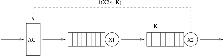
The lack of complete state information is reflected in the model by assuming that the input rate $\lambda$ is a function of only one of the $X_{i}$. If $\lambda(X)=\lambda(X_{1})$, then the analysis of the system can be reduced to the study of birth–death processes, which are well understood. This is why in the following it is always assumed that $\lambda(X)=\lambda(X_{2})$, so that the admission control introduces a feedback signaling loop to the system. For example, one can model a network where arriving traffic is rejected when the size of the second buffer exceeds a threshold level $K$ by setting $\lambda(X)=1(X_{2}\leq K)$, see Figure 1. In order to also cover more complex admission policies with multiple thresholds and thinning of input traffic, the shape of $\lambda(X_{2})$ will not be restricted in any way.

More precisely, $X$ is defined as a continuous-time stochastic process as follows. Let $\lambda$ be a nonnegative function on $\mathbb{Z}_{+}$ and $\mu_{1},\mu_{2}>0$. Define the transition rates $q(x,y)$ for $x\neq y$, $x,y\in\mathbb{Z}_{+}^{2}$ by

$$q(x,y)=\left\{\begin{aligned} \lambda(x_{2}),\quad&y=x+e_{1},\\ \mu_{1},\quad&y=x-e_{1}+e_{2}\geq 0,\\ \mu_{2},\quad&y=x-e_{2}\geq 0,\\ 0,\quad&\text{otherwise},\end{aligned}\right.$$

(1)

where $e_{i}$ denotes the $i$-th unit vector of $\mathbb{Z}_{+}^{2}$. As usual, set $q(x,x)=-q(x)$, where the transition rate out of state $x$ is defined by

$$q(x)=\sum_{y\neq x}q(x,y).$$

It is clear that $q(x)<\infty$ for all $x$, so using the minimal construction [3, 5] the rates $q(x,y)$ define a unique Markov process $X$ on $\mathbb{Z}_{+}^{2}\cup\{\kappa\}$. Here $\kappa$ denotes an additional state not in $\mathbb{Z}_{+}^{2}$ with $T_{\kappa}=\inf\{t>0:X(t)=\kappa\}\leq\infty$ being the time of explosion of $X$. The notation $S(\lambda,\mu_{1},\mu_{2})$ will be used for the set of transition rates corresponding to the the triple $(\lambda,\mu_{1},\mu_{2})$, and the system $S(\lambda,\mu_{1},\mu_{2})$ is said to be stable if the corresponding Markov process is ergodic, that is, irreducible and positive recurrent.

In its most general form, the stability problem may now be stated as

(P1)

Characterize the set of all $(\lambda,\mu_{1},\mu_{2})\in\mathbb{R}_{+}^{\mathbb{Z}_{+}}\times\mathbb{R}_{+}\times\mathbb{R}_{+}$ for which $S(\lambda,\mu_{1},\mu_{2})$ is stable.

Specializing to networks with threshold-based admission control, the offered traffic is assumed to arrive at unit rate, without loss of generality. Denoting the admission threshold by $K$, (P1) now takes the form

(P2)

For each $(\mu_{1},\mu_{2})\in\mathbb{R}_{+}^{2}$, determine for which values of $K\in\mathbb{Z}_{+}\cup\{\infty\}$, if any, the system $S(\,1(\cdot\leq K),\,\mu_{1},\mu_{2})$ is stable.

Note that the system corresponding to $K=\infty$ in (P2) is the ordinary tandem queue, for which it is well-known that $\min(\mu_{1},\mu_{2})>1$ is sufficient and necessary for stability. On the other hand, assuming overload, answering the question on the existence of a threshold level that can stabilize the system is not as straightforward.

The queueing systems literature includes a vast amount of work on various admission control mechanisms. However, most earlier studies on tandem networks require at least one of the buffers to be finite, so that the two-dimensional nature of the problem can partly be reduced to one-dimensional by applying matrix-geometric methods [9]. For networks with unlimited buffers and state-dependent service times, Bambos and Walrand [4] provide stability results extending to non-Markovian systems, however ruling out networks with the type of feedback signaling loop present here. Concerning the network $S(\lambda,\mu_{1},\mu_{2})$ defined above, the compensation approach introduced by Adan, Wessels, and Zijm [1] can be used for computing the invariant measure in the special case where $\lambda$ is constant on $\{n\in\mathbb{Z}_{+}:n\geq 1\}$. For more general input rates, Leskelä and Resing [7] have described a numerical method for calculating stationary performance characteristics of the system. Altman, Avrachenkov, and Núñez Queija [2] have recently introduced perturbation techniques that seem appropriate for asymptotically analyzing the behavior of $S(\lambda,\mu_{1},\mu_{2})$ under suitable parameter scaling.

This paper partially answers (P1) by deriving sufficient and necessary conditions for stability. Furthermore, by showing that in the special case of threshold-based admission control the sufficient and necessary conditions coincide, a complete solution of (P2) is given. In addition, the sensitivity of the system is analyzed with respect to changes in the service rates and it is shown how acceleration of one of the servers may, rather paradoxically, destabilize the system.

Let $S$ be a countable set. For a function $V:S\to\mathbb{R}$, denote

$$\lim_{x\to\infty}V(x)=\infty$$

if the set $\{x:V(x)\leq M\}$ is finite for all $M\in\mathbb{R}$. Further, the mean drift of $V$ with respect to transition rates $q(x,y)$ is denoted by

$$\Delta V(x)=\sum_{y\neq x}(V(y)-V(x))\,q(x,y),$$

(2)

assuming the sum on the right-hand side converges.

The following continuous-time analogue of Foster’s classical theorem [6] provides a sufficient condition for stability.

Considering the system $S(\lambda,\mu_{1},\mu_{2})$, let $q(x,y)$ be as defined in (1). Assume $V$ is a function on $\mathbb{Z}_{+}^{2}$ of the form $V(x)=x_{1}+v(x_{2})$ for some $v:\mathbb{Z}_{+}\to\mathbb{R}$ with $v(0)=0$. Searching for a Lyapunov function of this type, let us fix a number $r>0$ and require that the mean drift of $V$ with respect to $q$ satisfies

$$\Delta V(x)=-r\quad\text{for all $x$ with $x_{1}>0$}.$$

(3)

It is straightforward to verify that (3) is equivalent to

	$\displaystyle v(1)$	$\displaystyle=1-(\lambda(0)+r)/\mu_{1},$
	$\displaystyle v(n+1)$	$\displaystyle=1-(\lambda(n)+r)/\mu_{1}+(1+\mu_{2}/\mu_{1})v(n)-\mu_{2}/\mu_{1}v(n-1),\quad n\geq 1.$

Denoting $\alpha(n)=1-(\lambda(n)+r)/\mu_{1}$ and $w(n)=v(n+1)-v(n)$, the above difference equation can be written as $w(n)=\alpha(n)+\mu_{2}/\mu_{1}\,w(n-1)$ for $n\geq 1$, with $w(0)=\alpha(0)$. Thus, $w(n)=\sum_{k=0}^{n}\alpha(k)\,(\mu_{1}/\mu_{2})^{k-n}$, so that

$$v(n)=\sum_{j=0}^{n-1}w(j)=\sum_{j=0}^{n-1}\sum_{k=0}^{j}\alpha(k)\,(\mu_{1}/\mu_{2})^{k-j},$$

and we conclude that (3) defines for each $r>0$ the function

$$V_{r}(x)=x_{1}+\sum_{j=0}^{x_{2}-1}\sum_{k=0}^{j}(1-(\lambda(k)+r)/\mu_{1}))\,(\mu_{1}/\mu_{2})^{k-j}.$$

Thus we have constructed a family of functions $\mathcal{V}=\{V_{r}:r>0\}$ whose elements satisfy $\sup_{x:x_{1}>0}\Delta V_{r}(x)<0$, so there are hopes that $V_{r}$ might satisfy (F3) for a suitably chosen finite subset of $\mathbb{Z}_{+}^{2}$. In order to investigate whether this is the case, let us study the mean drift of $V_{r}$ for $x=(0,n)$ with $n\geq 1$,

$$\Delta V_{r}(0,n)=\lambda(n)-\mu_{2}(v_{r}(n)-v_{r}(n-1)).$$

(4)

In this paper, $Z_{n}$ and $Z$ will always represent generic random variables with distributions $\operatorname{geom}_{n}(\mu_{1}/\mu_{2})$ and $\operatorname{geom}(\mu_{1}/\mu_{2})$, respectively. Using this notation, one may verify that (4) can be alternatively written as

$$\Delta V_{r}(0,n)=\frac{\operatorname{E}\lambda(Z_{n})-\mu_{2}(1-r/\mu_{1})\,\operatorname{P}(Z_{n}>0)}{\operatorname{P}(Z_{n}=n)},\quad Z_{n}\sim\operatorname{geom}_{n}(\mu_{1}/\mu_{2}).$$

(5)

The proof of the theorem will utilize the following two lemmas.

Assume $\lambda(0)>0$ so that the system $S(\lambda,\mu_{1},\mu_{2})$ is irreducible. In the previous section we saw that

$$\varlimsup\operatorname{E}\lambda(Z_{n})<\min(\mu_{1},\mu_{2}),\quad Z_{n}\sim\operatorname{geom}_{n}(\mu_{1}/\mu_{2}),$$

is sufficient for the stability of $S(\lambda,\mu_{1},\mu_{2})$. This section is devoted to studying whether the above condition is also necessary for stability.

References

• [1] Adan, I. J. B. F., Wessels, J. and Zijm, W. H. M. (1993). Compensation approach for two-dimensional Markov processes. Adv. Appl. Probab. 25, 783–817.
• [2] Altman, E., Avrachenkov, K. E. and Núñez Queija, R. (2004). Perturbation analysis for denumerable Markov chains with application to queueing models. Adv. Appl. Probab. 36, 839–853.
• [3] Asmussen, S. (2003). Applied Probability and Queues second ed. Springer.
• [4] Bambos, N. and Walrand, J. (1989). On stability of state-dependent queues and acyclic queueing networks. Adv. Appl. Probab. 21, 618–701.
• [5] Brémaud, P. (1999). Markov Chains: Gibbs Fields, Monte Carlo Simulation, and Queues. Springer.
• [6] Foster, F. G. (1953). On the stochastic matrices associated with certain queuing processes. Ann. Math. Statist. 24, 355–360.
• [7] Leskelä, L. and Resing, J. (2007). A tandem queueing network with feedback admission control. In Proc. First EuroFGI International Conference NET-COOP. ed. T. Chahed and B. Tuffin. vol. 4465 of LNCS. Springer. pp. 129–137.
• [8] Meyn, S. P. and Tweedie, R. L. (1993). Markov Chains and Stochastic Stability. Springer.
• [9] Neuts, M. F. (1981). Matrix-Geometric Solutions in Stochastic Models. John Hopkins University Press.
• [10] Tweedie, R. L. (1975). Sufficient conditions for regularity, recurrence and ergodicity of Markov processes. Math. Proc. Cambridge 78, 125–136.
Acknowledgements
This work was funded by the Academy of Finland Teletronics II / FIT project and the Finnish Graduate School in Stochastics. The author would like to thank Ilkka Norros for his valuable help and advice during the project, Jarmo Malinen for many inspiring discussions, and the anonymous referee for helpful comments on improving the presentation of the results.