Aggregation Languages for Moving Object and Places of Interest Data
Abstract
We address aggregate queries over GIS data and moving object data, where non-spatial data are stored in a data warehouse. We propose a formal data model and query language to express complex aggregate queries. Next, we study the compression of trajectory data, produced by moving objects, using the notions of stops and moves. We show that stops and moves are expressible in our query language and we consider a fragment of this language, consisting of regular expressions to talk about temporally ordered sequences of stops and moves. This fragment can be used to efficiently express data mining and pattern matching tasks over trajectory data.
1 Introduction
Geographic Information Systems (GIS) have been extensively used in various application domains, ranging from economical, ecological and demographic analysis, to city and route planning [17, 23]. In recent years, time is playing an increasingly important role in in GIS and spatial data management [14]. One particular line of research in this direction, introduced by Wolfson [4, 5, 12, 21, 22, 19], concerns moving object data. Moving objects, carrying location-aware devices, produce trajectory data in the form of a sample of -tuples, that contain object identifier and time-space information.
In this paper, we are interested in aggregate queries over GIS data and moving object data. Typically, when aggregation becomes important, it is advisable to organize the non-spatial data in a GIS in a data warehouse. In a data warehouse, numerical data are stored in fact tables built along several dimensions. For instance, if we are interested in the sales of certain products in stores in a given region, we may consider the sales amounts in a fact table over the three dimensions store, time and product. In general dimensions are organized into aggregation hierarchies. For example, stores can aggregate over cities which in turn can aggregate into regions and countries. Each of these aggregation levels can also hold descriptive attributes like city population, the area of a region, etc. For traditional alpha-numeric data, OLAP (On Line Analytical Processing) [10] comprises a set of tools and algorithms that allow efficiently querying multidimensional databases, containing large amounts of data, usually called data warehouses.
Two of the present authors have proposed in previous work a model for smoothly integrating the GIS and OLAP worlds. This model was implemented using open source software [6]. The same authors also proposed a taxonomy of aggregation queries on moving object data [11]. In this paper, we propose a conceptual model and a formal query language that cover the different types of aggregation queries discussed in the above mentioned taxonomy (see Sections 2 and 3). At the basis of our aggregation query language is a multi-sorted first-order query language for moving object and GIS data in which one can specify properties of moving objects, geometric elements of GIS layers and OLAP data storing the non-spatial GIS data.
Recently, in the study of moving object data, the concepts of stops and moves were introduced [13, 2]. These concepts serve to compress the trajectory data that is produced by moving objects using application dependent places of interest. A designer may want to select a set of places of interest that are relevant to her application. For instance, in a tourist application, such places can be hotels, museums and churches. In a traffic control application, they may be road segments, traffic lights and junctions. We assume that these places of interest are stored in a specific GIS layer. If a moving object spends a sufficient amount of time in a place of interest, this place is considered a stop of the object’s trajectory. In between stops, the trajectory has moves. Thus, we can replace a raw trajectory given by -tuples by a sequence of application-relevant stops and moves. In this paper, we give a geometric definition of stops and moves and show that they are computable (see Section 4). We also show that this compression can be expressed in the language and we sketch a sublanguage of that allows us to talk about temporally ordered sequences of stops and moves (see Section 5). The syntax of this languages is given in the form of regular expressions (see Section 6). We show that this language considerably extends the language proposed by Mouza and Rigaux [13], and can be used to efficiently express data mining and pattern matching tasks over trajectory data.
1.1 Running Example
Now, let us introduce the example we will be using throughout the paper. Figure 1 (left) shows a simplified map of Paris, containing two hotels, denoted Hotel 1 and Hotel 2 (H1 and H2 from here on), the Louvre and the Eiffel tower. We consider three moving objects, O1, O2 and O3. Object O1 goes from H1 to the Louvre, the Eiffel tower, spends just a few minutes there, and returns to the hotel. Object O2 goes from H1 to the Louvre, the Eiffel tower (it stays a couple of hours in each place), and returns to the hotel. Object O3 leaves H2 to the Eiffel tower, visits the place, and returns to H2. Figure 1 shows an example of these trajectory samples on the right.
In this scenario, a GIS user may be interested in finding out useful trajectory information in this setting, like “number of persons going from H1 to the Louvre and the Eiffel tower (visiting both places) in the same day”, or “number of persons going from a hotel in the left bank of the Seine, to the Louvre in the mornings”.
 1
2
1
4
2
3
4
5
6
3
2
3
1
2
1
4
2
3
4
5
6
3
2
3
1.2 Related Work
GIS and OLAP Interaction
Although some authors have pointed out the benefits of combining GIS and OLAP, not much work has been done in this field. Vega López et al [20] present a comprehensive survey on spatiotemporal aggregation that includes a section on spatial aggregation. Rivest et al. [18] introduce the concept of SOLAP (standing for Spatial OLAP), and describe the desirable features and operators a SOLAP system should have. Han et al. [7] used OLAP techniques for materializing selected spatial objects, and proposed a so-called Spatial Data Cube. This model only supports aggregation of such spatial objects.
Moving Objects
Many efforts have been made in the field of moving objects databases, specially regarding data modeling an indexing. Güting and Schneider [5] provide a good reference to this large corpus of work. Güting et al proposed a system of abstract data types as extensions to DBMSs to support time-dependant geometries [4]. Hornsby and Egenhofer [8] introduced a framework for modeling moving objects, that supports viewing objects at different granularities, depending on the sampling time interval. The possible positions of an object between two observation is estimated to be within two inverted half-cones that conform a lifeline bead, whose projection over the x-y plane is an ellipse. Another approach to moving objects studies moving objects on networks, basically represented as graphs. Van de Weghe et al proposed a qualitative trajectory calculus for objects in a GIS [3], based on the assumption that in a GIS scenario, qualitative information is necessary (and, in general, more useful than quantitative information).
Aggregate information is still quite an open field, either in GIS or in a moving objects scenario. Meratnia and de By [12] have tackled the topic of aggregation of trajectories, identifying similar trajectories and merging them in a single one, by dividing the area of study into homogeneous spatial units. Papadias et al [15] index historical aggregate information about moving objects. They aim at building a spatio-temporal data warehouse
Regarding the addition of semantics to trajectories, Brakatsoulas et al[1], in the context of trajectory mining in road networks, propose to enrich trajectories of moving objects with information about the relationships between trajectories (e.g., intersect, meets), and between a trajectory and the GIS environment (stay within, bypass, leave). Extending this notion, Damiani et al [2] introduced the concept of stops and moves, in order to enrich trajectories with semantically annotated data. With a similar idea, [13] propose a model where trajectories are represented by a sequence of moves. They propose a query language based on regular expressions, aimed at obtaining so-called mobility patterns. However, this language is only geared towards trajectory data, and does not relate trajectories with the GIS environment. Thus, the classes of queries addressed is limited. Moreover, aggregation is not considered in this language.
We can conclude that, although the efforts above address particular problems, integrating spatial and warehousing information in a single framework is still in its infancy.
2 A Data Model for Moving Objects
Our work is based on the data model introduced in [6, 11]. In this section we give an overview of this model. We first present the model for spatial data, and then we introduce the notion of moving objects.
2.1 Spatial Data
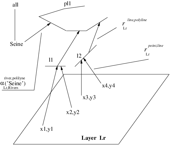
A GIS dimension is considered, as usual in databases, as composed of a schema and instances. Figure 2 (left) depicts the schema of a GIS dimension: the bottom level of each hierarchy, denoted the Algebraic part of the dimension, contains the infinite points in a layer, and could be described by means of linear algebraic equalities and inequalities [16]. Above this part there is the Geometric part, that stores the identifiers of the geometric elements of GIS and is used to solve the geometric part of a query (i.e. find the polylines -implemented as linestrings- in a river representation). Each point in the Algebraic part may correspond to one or more elements in the Geometric part. Thus, at the GIS dimension instance level we will have rollup relations (denoted These relations map, for example, points in the Algebraic part, to geometry identifiers in the Geometric part For example, says that point corresponds to a polygon identified by in the Geometric part (note that a point may correspond to more than one polygon, o to more than one polylines that intersect with each other).
Finally, there is the OLAP part of the dimension. This part contains the conventional OLAP structures, as defined in [9]. The levels in the geometric part are associated to the OLAP part via a function, denoted For instance, associates information about a river in the OLAP part (), to the identifier of a polyline () in a layer containing rivers () in the Geometric part.
 |
 |
Example 1
Figure 2 (left) shows a GIS dimension schema, where we defined three layers, for rivers, cities, and provinces, respectively. The schema is composed of three graphs; the graph for rivers contains edges saying that a point in the algebraic part relates to a line identifier in the geometric part, and that in the same portion of the dimension, this line aggregates on a polyline identifier.
In the OLAP part we have information given by two dimensions, representing districts and rivers, associated to the corresponding graphs, as the figure shows. For example, a river identifier at the bottom layer of the Rivers dimension representing rivers in the OLAP part, is mapped to the polyline dimension level in the geometric part in the graph in the rivers layer .
Figure 2 (right) shows a portion of a GIS dimension instance of the rivers layer in the dimension schema of the schema in the left of the figure. Here, an instance of a GIS dimension in the OLAP part is associated to the polyline which corresponds to the Seine river. For simplicity we only show four different points at the level There is a relation containing the association of points to the lines in the line level, and a relation between the line and polyline levels, in the same layer. ∎
Elements in the geometric part can be associated with facts, each fact being quantified by one or more measures, not necessarily a numeric value. Of course, besides the GIS fact tables, there may also be classical fact tables in the OLAP part, defined in terms of the OLAP dimension schemas. For instance, we could either store the population associated to a polygon identifier, or in a data warehouse fact table, with schema
2.2 Moving Object Data Representation
Besides the static information representing geometric components (i.e., the GIS), for representing time in the OLAP part there will be a Time dimension (actually, there could be more than one Time dimensions, supporting, for example, different notions of time). Also, as it is well-known in OLAP, this time dimension can have different configurations that depend on the application at hand. Moving objects are integrated in the former framework using a distinguished fact table denoted Moving Object Fact Table (MOFT).
First, we say what a trajectory is. In practice, trajectories are available by a finite sample of points, obtained by observation.
Definition 1 (Trajectory)
A trajectory is a list of time-space points , where for and . We call the interval the time domain of the trajectory. ∎
For the sake of finite representability, we may assume that the time-space points , have rational coordinates.
A moving object fact table (MOFT for short, see the table in the right hand side of Figure 1 contains a finite number of identified trajectories. Formally:
Definition 2 (Moving Object Fact Table)
Given a finite set of trajectories, a Moving Object Fact Table (MOFT) for is a relation with schema where is the identifier of the moving object, represents time instants, and and represent the spatial coordinates of the objects. An instance of the above schema contains a finite number of tuples of the form , that represent the position of the object at instant for the trajectories in .∎
3 A Query Language for Aggregation of Moving Object Data
The aggregation queries that we address in this paper are based on a first-order moving object query language and they are of the following types:
- –
the Count operator applied to sets of the form where moving objects identifiers satisfying some -definable property are collected;
- –
the Count operator applied to sets of the form where moving objects identifiers combined with time moments, satisfying some -definable property , are collected (assuming that this set is finite; otherwise the count is undefined);
- –
the Count operator applied to sets of the form where moving objects id’s combined with time and space coordinates, satisfying some -definable property , are collected (assuming that this set is finite);
- –
the Area operator applied to sets of the form which define some -definable part of the plane (assuming that this set is linear and bounded);
- –
the Count, Max and Min operators applied to sets of the form when the -definable condition defines a finite set of time instants and the TimeSpan operator when defines an infinite, but bounded set of time instants (the semantics of Count, Max and Min is clear and TimeSpan returns the difference between the maximal and minimal moments in the set);
- –
the Max-l, Min-l, Avg-l and TimeSpan-l operators applied to sets of the form which represents an -definable set of time intervals. The meaning of these operators is respectively the maximum, minimum and average lengths of the intervals if there is a finite number of intervals and the timespan of the union of these intervals in the last case;
- –
the Area operator applied to sets of the form where identifiers of elements of some geometry (in the geometric part of our data model), satisfying an -definable are collected. The meaning of this operator is the total area covered by the geometric elements corresponding to the identifiers.
Obviously, the above list is not complete, but is covers the most interesting and usual cases (see [11] for an extensive list of examples of moving object aggregation queries). For instance, sets like do not correspond to any obvious entity we would like to aggregate over.
To complete the description of our moving-object aggregation language, the query language remains to be defined. In the -definable sets considered above, we can see that there are variables of different kinds, like and In fact, is a multi-sorted first-order logic using variables of these types to define sets as considered above. We now define more formally.
Definition 3
The first-order query language has four types of variables: real variables ; name variables ; geometric identifier variables and dimension level variables (which are also use for dimension level attributes).
Besides (existential and universal) quantification over all these variables, and the usual logical connectives , we consider the following functions and relations to build atomic formulas in :
- –
for every rollup function in the OLAP part, we have a function symbol , where and are geometries and is a dimension;
- –
analogously, for every rollup relation in the GIS part, we have a relation symbol , where and are geometries and is a layer;
- –
for every relation associating the OLAP and GIS parts in some layer , we have a relation symbol , where is a OLAP dimension level and is a geometry, is a layer and is a dimension;
- –
for every dimension level A, and every attribute of denoted there is a function that maps elements of to elements of in dimension ;
- –
we have functions, relations and constants that can be applied to the alpha-numeric data in the OLAP part (e.g., we have the relation to say that an element belongs to a dimension level, we may have on income values and the function on string values);
- –
for every MOFT, we have a 4-ary relation ;
- –
we have arithmetic operations and the constants and , and the relation for real numbers.
- –
finally, we assume the equality relation for all types of variables.
If needed, we may also assume other constants, e.g., for object identifiers. ∎
Definition 3 describes the syntax of the language . The interpretation of all variables, functions, relation, and constants is standard, as well as that of the logical connectives and quantifiers. We don’t define the semantics formally but illustrate through an elaborate example.
Example 2
Let us consider the query “Give the total number of buses per hour in the morning in the Paris districts with a monthly income of less than C 1500,00.”
We use the MOFT (Figure 1, left), that contains the moving objects samples. For clarity, we will denote the geometry polygons by , polylines by and point by . We use distr to denote the level district in the OLAP part of the dimension schema. The GIS layer which contains district information is called . As in the above definition, we assume that the layers to which a function refers are implicit by the function’s name. For instance, in the expression , the district variable is mapped to the polygon with variable name that is in the layer , indicated by the function (here is a dimension in the OLAP part representing districts). Thus, the result of the query returning the region with the required income is expressed as:
In this expression, relates points to polygons in the district layer; the function maps the district identifier in the OLAP part to the geometry identifier ; and maps the district identifier to the value of the income attribute which then is compared by an OLAP relation with a OLAP constant .
The instants corresponding to the morning hours mentioned in the fact tables are obtained through the rollup functions in the Time dimension. We assume in the Time dimension a category denoted timeOfDay, rolling up to the dimension category hour (i.e., ). The aggregation of the values in the fact table corresponding only to morning hours is computed with the following expression: In this formula “Morning” appears as a constant related to the OLAP part. Finally, the query we discuss reads:
|
|
If we would change the given aggregation query to “Give the total number of buses per hour in the morning within 3 km from a Paris district with a monthly income of less than C 1500,00.” then we would need , and to express the distance constraint. This would introduce a quadratic polynomial in the formula to express that some points are less than 3 km apart. This concludes the example.∎
Proposition 1
Moving object queries expressible in are computable. The proposed aggregation operators are also computable.
Proof
(Sketch) The semantics of expressions is straightforward apart from the subexpressions that involve , and on real numbers and quantification over real numbers. These subexpressions belong to the formalism of constraint databases and they can be evaluated by quantifier elimination techniques [16].
The restrictions that we imposed on the applicability of the aggregation operators make sure that they can be effectively evaluated. In particular, the area of a set is computable when this set is semi-linear and bounded. This area can be obtained by triangulating such linear sets and adding the areas of the triangles.∎
4 Stops and Moves of Trajectories
In this section, we define what the stops and moves of a trajectory are. In a GIS scenario, this definition is dependent on the particular places of interest in a particular application. For instance, in a tourist application, places of interest may be hotels, museums and churches. In a traffic application, places of interest may be road segments, road junctions and traffic lights. First, we define the notion of “places of interest of an application” (PIA).
Definition 4
[Places of Interest] A place of interest (PoI) is a tuple , where is a (topologically closed) polygon, polyline or point in and is a strictly positive real number. The set is called the geometry of the PoI and is called its minimum duration.
The places of interest of an application (PIA) is a finite collection of PoIs with mutually disjoint geometries.∎
Definition 5
[Stops and moves of a trajectory] Let be a trajectory and let be a PIA.
A stop of with respect to is a maximal contiguous subtrajectory of such that for some the following holds: (a) for ; (b) .
A move of with respect to is: (a) a maximal contiguous subtrajectory of in between two temporally consecutive stops of ; (b) maximal contiguous subtrajectory of in between the starting point of and the first stop of ; (c) a maximal contiguous subtrajectory of in between the last stop of and ending point of ; (d) the trajectory itself, if has no stops. ∎
Figure 3 illustrates these concepts. In this example, there are four places of interest with geometries and . The trajectory is depicted here by linearly interpolating between its sample points, to indicate their order. Let us imagine that is run through from left to right. If the three sample points in are temporally far enough apart (longer than ), they form a stop. Imagine that further on, only the two sample points in are temporally far enough apart to form a stop. Then we have two stops in this example and three moves.
We remark that our definition of stops and moves of a trajectory is arbitrary and can be modified in many ways. For example, if we would work with linear interpolation of trajectory samples, rather than with samples, we see in Figure 3, that the trajectory briefly leaves (not in a sample point, but in the interpolation). We could incorporate a tolerance for this kind of small exists from PoIs in the definition, if we define stops and moves in terms of continuous trajectories, rather than on terms of samples. The following property is straightforward.
Proposition 2
There is an algorithm that returns, for any input with a PIA and a trajectory , the stops of with respect to . This algorithm works in time , where is the complexity of answering the point-query [17]. ∎
5 A Stops and Move Fact Table
Let the places of interest (PoIs) of an application (PIA) be given. In this section, we describe how we go from MOFTs to application dependent compressed MOFTS, where tuples are replaced by tuples. In the latter tuples, is a moving object identifier, is an identifier of the geometry of a place of interest and and are two time moments that encode the time interval of a stop. The idea is to replace the trajectories in a MOFT that are stored there as samples, by a stops MOFT that represents the same trajectory more concisely by listing its stops and the time intervals spent in the stops.
In our model, application information about the PoIs is stored in the OLAP part as OLAP dimensions. For example, if hotels are places of interest, we will need to create a dimension Hotels such that its bottom level contains the identifier for the hotels and some hierarchy that is specific for hotels, e.g., a hotel may belong to the 3-star category. Given that these dimensions depend on a particular application, we define, at the conceptual level, a Generic virtual dimension, from which different dimensions can be generated.
To start with, we assume that the places of interest are stored in moving object OLAP in the following way: the geometries of the PoIs are represented in a layer in the GIS denoted (e.g., a layer containing polygons that represent hotels or a layer containing polylines that represent street segments). Data describing the places of interest is stored in the OLAP part.
Figure 4 illustrates how the information about the places of interest is represented in our model. In this figure, in the OLAP part there is a virtual dimension, which we call the Generic PoI, that will be instantiated by as many types of places of interest as a particular application requires (in the figure, we show an instantiation for hotels). The bottom level of this dimension is denoted There is also a function that maps the bottom level of the instances of the Generic PoI (GPoI) to geometries in the geometric part, in the layer corresponding to the PoIs, denoted . In Figure 4, hotelId is mapped to the geometry Polygon in the layer . The minimum duration of a PoI is stored as an attribute of the bottom level of the instances of the GPoI. For example, an attribute of level hotelId in Figure 4. At the instance level, analogous to what we explained in Section 2, the function maps elements in the bottom level () of the instances of the GPoI, to the geometric identifiers of the places of interest in the geometric part (in Figure 4, the function is defined as ).

.
Definition 6 (SM-MOFT)
Let be a PIA of PoIs and let be a MOFT. The SM-MOFT of with respect to consist of the tuples such that (a) is the identifier of a trajectory in ; (b) is the identifier of the geometry of a PoI of such that the trajectory with identifier in has a stop in this PoI during the time interval . This interval is called the stop interval of this stop. ∎
The table in Figure 5 (left) gives an example of a SM-MOFT. The following property shows that SM-MOFTs can be defined in the moving object query language .
Proposition 3
There is an formula that defines the SM-MOFT of with respect to . ∎
We omit the proof of this property but remark that the use of the formula allows us to speak about stops and moves of trajectories in . We can therefore add predicates to define stops and moves of trajectories as syntactic sugar to .
6 A Query Language for Moving Objects
In this section we will show how the language and the model supporting it, can yield sub-languages that can address many interesting aggregation queries for moving objets in a GIS environment. We will sketch a query language based on path regular expressions, along the lines proposed by [13]. However, our language goes far beyond, taking advantage of the integration between GIS, OLAP and moving objects provided with our model. Moreover, queries that do not require access to the MOFT can be evaluated very efficiently, making use of the SM-MOFT.
The idea is based on the construction of a graph representing the stops and moves of a single trajectory as follows: from the SM-MOFT we construct a graph as follows. For each different in there is a node in denoted which is assigned a unique node number . Further, there is an edge in between two nodes and for every pair of of consecutive tuples in with the same Each node is augmented with two functions and one set: (a) the function returns the identifier of the PoI in the OLAP part of the model (i.e., the such that ); (b) the function returns the dimension in the OLAP part to which a given PoI belongs (v.g, Hotels, Museums, and so on); (c) a set of Stop Intervals (technically a temporal element) STE(v), containing the stop intervals of the object at Note that an object may be at a stop more than one time within a trajectory. Further, these is an ordered set, given that the intervals are disjoint by definition and consecutive by construction. We denote the graph constructed in this way an SM-Graph.
Example 3

We will also need some operators on time intervals. We say that an interval strictly precedes denoted if We also say that returns True if Note that all stop intervals of the same trajectory are such that either or
Now we are ready to define a simplified query language for moving object aggregation, taking advantage of the concept of stops and moves, but powerful enough to combine (to some extent) the notion of regular path expressions and first order constraints. We assume that MOFTs are well-defined, thus the graphs are temporally consistent. In addition, each edge in an SM-Graph is univocally defined by the intervals of the stop temporal elements of the beginning and ending nodes of the edge. In other words, if there exist two edges from a node to a node Each node must have associated two stop temporal intervals, and where holds.
A first observation at the definition of the -Graph reveals that the graph can be seen as a DFA accepting regular expressions over the labels of the nodes in the graph. This becomes clear if, in the graph of Figure 5 (right) we replace by . In this case, the nodes labeled and will become and respectively (shorthand for Museums and Hotels. We call this graph ASM-Graph (the A stands for aggregation). As a second observation, we can think on a language such that the DFA accepting this language is contained in the ASM-Graph. Thus, a trajectory satisfies a query if the DFA of the query is contained in
Definition 7 (Regular Expressions Language for Stops and Moves)
An regular expression on stops and moves, denoted RESM is an expression generated by the grammar
where (a set of dimension names in the OLAP part), is the symbol representing the empty expression, “.” means concatenation, and represents a condition over . The term “?” is a wildcard meaning “any sequence of any number of ”.∎
The aggregate language is built on top of RESMs: for each trajectory in an SM-MOFT such that there is a sub-trajectory of that matches the RESM, the query returns the of Then, we can apply the aggregate function Count to the set returned.
We explain the semantics of RESM-based language using the query: “total number of trajectories that went from a “Hilton” hotel to a tourist attraction, stopping at a museum.”, whose RESM reads: Count(H[name=‘Hilton’].?.M.?.T).
Note that “name” is an attribute of the PoI identifier in the OLAP part (an attribute of the extension of the node). Then, for each trajectory, and for each instantiation with a value H, M or T, of a node in the graph, the variable is instantiated with the value corresponding to the attribute of in the OLAP part such that in the dimension The condition on the node is then checked. Finally, if there is a sub-trajectory matching the RESM, then its counts for the aggregation.
As another example, the query “total number of trajectories that
went from a Hilton hotel to the Louvre, in the morning.”
Count(H[name=’Hilton’].?.M[name=’Louvre’ ])
The semantics of the first condition is analogous to the semantics of the query above. The same occurs with the condition over in M. For the last part of the condition over M, for each trajectory, and each instantiation of a node in the graph with a value or , is instantiated with values of
Proposition 4
The language defined above is a subset of ∎
Proof
(Sketch) The proof is built on the property that, for each trajectory in an SM-MOFT the SM-Graph can be unfolded, and transformed into a sequence of nodes, given that for all nodes in the graph, all intervals in are disjoint. Thus, this sequence can then be queried using any FO language with time variables, like ∎
7 Future Work
Our future work will be focused in the implementation of the model and query languages proposed here, and its integration with the framework introduced in [6]. We also believe that the RESM language is promising for mining trajectory data, specifically in the context of sequential patterns mining with constraints, and we will work in this direction.
References
- [1] S. Brakatsoulas, D. Pfoser, and N. Tryfona. Pre-aggregation in spatial data warehouses. In Proceedings of IDEAS’04, pages 68–77, Washington D.C, USA, 2004.
- [2] M. L. Damiani, J. A. Fernandes de Macedo, C. Parent, F. Porto, and S. Spaccapietra. A conceptual view of trajectories. Technical Report, Ecole Polythecnique Federal de Lausanne, April 2007, 2007.
- [3] N. Van de Weghe, A. Cohn, G. De Tré, and P. De Maeyer. A qualitative trajectory calculus as a basis for representing moving objects in geographical information systems. Control and Cybernetics (to appear), 2005.
- [4] R. H. Güting, M. H. Böhlen, M. Erwig, C. S. Jensen, N. A. Lorentzos, M. Schneider, and M. Vazirgiannis. A foundation for representing and quering moving objects. ACM Trans. Database Syst., 25(1):1–42, 2000.
- [5] R. H. Güting and M. Schneider. Moving Objects Databases. Morgan Kaufman, 2005.
- [6] S. Haesevoets, B. Kuijpers, and A. Vaisman. Spatial aggregation: Data model and implementation. In Submitted for review, 2006.
- [7] J. Han, N. Stefanovic, and K. Koperski. Selective materialization: An efficient method for spatial data cube construction. In Proceedings of PAKDD’98, pages 144–158, 1998.
- [8] K. Hornsby and M. Egenhofer. Modeling moving objects over multiple granularities. Special issue on Spatial and Temporal Granularity, Annals of Mathematics and Artificial Intelligence, 2002.
- [9] C. Hurtado, A.O. Mendelzon, and A. Vaisman. Maintaining data cubes under dimension updates. In Proceedings of IEEE/ICDE’99, pages 346–355, 1999.
- [10] R. Kimball and M. Ross. The Data Warehouse Toolkit: The Complete Guide to Dimensional Modeling, 2nd. Ed. J.Wiley and Sons, Inc, 2002.
- [11] B. Kuijpers and Alejandro Vaisman. A data model for moving objects supporting aggregation. In Proceedings of the First International Workshop on Spatio-Temporal Data Mining (STDM’07), Istambul, Turkey, 2007.
- [12] N. Meratnia and R. de By. Aggregation and comparison of trajectories. In Proceedings of the 26th VLDB Conference, Virginia, USA, 2002.
- [13] C. Mouza and P. Rigaux. Mobility patterns. Geoinformatica, 9(23):297–319, 2005.
- [14] Th. Ott and Fr. Swiaczny. Time-integrative Geographic Information Systems–Management and Analysis of Spatio-Temporal Data. Springer, 2001.
- [15] D. Papadias, Y. Tao, J. Zhang, N. Mamoulis, Q. Shen, and J. Sun. Indexing and retrieval of historical aggregate information about moving objects. IEEE Data Eng. Bull., 25(2):10–17, 2002.
- [16] J. Paredaens, G. Kuper, and L. Libkin, editors. Constraint databases. Springer-Verlag, 2000.
- [17] P. Rigaux, M. Scholl, and A. Voisard. Spatial Databases. Morgan Kaufmann, 2002.
- [18] S. Rivest, Y. Bédard, and P. Marchand. Modeling multidimensional spatio-temporal data warehouses in a context of evolving specifications. Geomatica, 55 (4), 2001.
- [19] M. Vazirgiannis and O. Wolfson. A spatiotemporal model and language for moving objects on road networks. In SSTD, pages 20–35, 2001.
- [20] I. Vega López, R. Snodgrass, and B. Moon. Spatiotemporal aggregate computation: A survey. IEEE Transactions on Knowledge and Data Engineering 17(2), 2005.
- [21] O. Wolfson, P. Sistla, B. Xu, and S. Chamberlain. Domino: Databases fOr MovINg Objects tracking. In Proceedings of SIGMOD’99, pages 547 – 549, 1999.
- [22] O. Wolfson, B. Xu, S. Chamberlain, and L. Jiang. Moving objects databases: Issues and solutions. In SSDBM, pages 111–122, 1998.
- [23] M. F. Worboys. GIS: A Computing Perspective. Taylor&Francis, 1995.