Theory and Phenomenology of Exotic Isosinglet Quarks and Squarks
Abstract
Extensions of the MSSM often predict the existence of new fermions and their scalar superpartners which are vectorlike with respect to the standard model gauge group but may be chiral under additional gauge factors. In this paper we explore the production and decay of an important example, i.e., a heavy isosinglet charge quark and its scalar partner, using the charge assignments of a -plet of for illustration. We emphasize that, depending on the symmetries of the low energy theory, such exotic particles may decay by the mixing of the fermion with the , or quarks; may decay by leptoquark or diquark couplings (which may nevertheless preserve a form of -parity); or may be stable with respect to renormalizable couplings but decay by higher-dimension operators on cosmological times scales. We discuss the latter two possibilities in detail for various assumptions concerning the relative masses of the exotic fermions, scalars, and the lightest neutralino, and emphasize the necessity of considering the collider signatures in conjunction with the normal MSSM processes. Existing and projected constraints from colliders, indirect experiments, proton decay, and big bang nucleosynthesis are considered.
pacs
12.60.Jv,04.65.+e,14.80.Ly,95.35.+dI Introduction
As the beginning of data-taking at the CERN Large Hadron Collider (LHC) rapidly approaches, there has been an increase in research into both the possible new physics opportunities as well as the challenges facing experimenter and theorist alike. The focus of attention has thus far been squarely on new physics of a supersymmetric nature, in particular on the minimal supersymmetric extension of the Standard Model (MSSM). This is undoubtedly a well-justified approach, but in our preparatory studies of opportunities and challenges at the LHC it is wise to sometimes take a broader view of what the TeV scale may reveal. There has recently been a growing appreciation Binetruy:2003cy; Allanach:2004my; Datta:2005vx; Allanach:2005kz; Arkani-Hamed:2005px; Plehn:2004rp of the possible difficulties in connecting data to underlying theories, focusing on extracting parameters of the MSSM Lagrangian or distinguishing the MSSM from some other paradigm of new particle physics. In this paper we wish to consider another possibility. We will consider here the case in which the “usual” new physics signal from the states of the MSSM is combined with that from additional supersymmetric states accessible at the TeV scale. In particular, we will consider the presence of additional vector-like pairs of triplets which are singlets under the of the Standard Model but carry non-vanishing hypercharge (as well as possible additional charges).
Such states, which we will denote as and in this work, are among the most well-motivated extensions of the MSSM particle content. For example the supersymmetric , and grand unified theories (GUTs), as well as non-supersymmetric , predict the existence of such states Langacker:1980js; Hewett:1988xc, though only in the case (or in nonminimal versions of and ) can some of them have electroweak-scale masses without severely compromising the lifetime of the proton. Simple enlargements of the electroweak sector of the MSSM incorporate these states, to saturate anomaly cancelation constraints in models and/or to contribute to the radiative breaking of the extended symmetries Cvetic:1995rj; Cvetic:1997ky; Keith:1997zb; Langacker:1998tc; Daikoku:2000ep; Erler:2000wu. extensions11 1 Such extensions are consistent with simple gauge coupling unification if the and occur in combination with additional vector-like Higgs or lepton doublet pairs, i.e., so that the new states have the quantum numbers of a of . may arise, for example, as variations on the NMSSM Ellis:1988er for generating dynamical terms. Structures of these sorts arise routinely in top-down string constructions, particularly those of the heterotic string Antoniadis:1986rn; Kawai:1986va; Kawai:1986vd; Antoniadis:1989zy; Faraggi:1993pr; Chaudhuri:1994cd; Cleaver:1998gc; Cleaver:1999cj; Giedt:2001zw – so much so, in fact, that the -version of and are often referred to simply as ‘‘superstring-inspired’’ exotics.22 2 In explicit string constructions one finds that additional triplets/antitriplets of often have charges that distinguish these states from their GUT counterparts. Yet more significant (for our purposes) than these motivations is the simple fact that the existence of additional vector-like pairs of triplets is a very real logical possibility that will have a significant impact on the experimental environment at a hadron collider such as the LHC.33 3 In this regard the present work serves as a complement to similar treatments of new doublets and new Higgs singlets Ellis:1988er; nMSSM; Panagiotakopoulos:2000wp; Menon:2004wv; Dermisek:2005ar; Ellwanger:2005uu; Barger:2006dh; O'Connell:2006wi; Barger:2006sk; Dermisek:2007yt; Barger:2007im or other types of new physics Barger:2007ay at the LHC.
Consider, for example, the various logical possibilities for interaction between exotic and states and the fields of the Standard Model. The simplest scenario, and the one that is usually studied, especially in the non-supersymmetric case, is one in which the exotic and the Standard Model are allowed (by the conserved quantum numbers) to mix, as are the conjugate fields and . Another scenario might forbid this sort of mixing (e.g., because of R-parity conservation), but allow renormalizable interactions between the new , and Standard Model fields in the superpotential. Depending on the quantum numbers of the exotic states a range of possible production and decay mechanisms would then be operative, including interactions that are leptoquark or diquark in nature. Still another possibility is that some new symmetry – or combination of symmetries – forbids these renormalizable interactions but allows higher-order interactions in the superpotential. In this case the new exotics would be “quasi-stable”; they would have a lifetime that implies stability on collider timescales (approximately 100ns or longer) but might decay sufficiently quickly to avoid cosmological limits on such objects. Finally, we mention the possibility that the exotic particle is absolutely stable or stable on the time scale of the age of the universe. This would imply cosmological difficulties and is also severely constrained by searches for heavy stable particles, e.g., in sea water (for a review, see Perl:2001xi). However, these difficulties could possibly be avoided if the reheating temperature of the universe after inflation was very low Giudice:2000ex, especially if the mass is larger than a TeV Kudo:2001ie.
In this work we will therefore cover a variety of such phenomena: new signatures and new challenges for connecting data to theories, cosmological issues of long-lived heavy -charged states, and indirect constraints coming from limits on rare processes. The goal is to be as comprehensive as possible in enumerating all the logically distinct ways in which these exotic quarks and squarks can manifest themselves in Nature. In each case we wish to ask what are the constraints on the existence of these new states, and by what observational methods will we infer their existence? We would also like to know how the answers to these questions will depend on the free parameters of theories which contain such exotics. To this end we will need to consider an array of possibilities instead of any one paradigm. Nevertheless, to be concrete, one needs to discuss phenomena in terms of a model or class of models. We will therefore choose representative ones when necessary, but we strive to treat everything as model-independently as is possible. We note that several specific models that fall into this class have already been studied at length, but other aspects which we cover have hardly been mentioned in the literature. More complete references to existing studies will be provided in the appropriate sections.
The rest of the paper is organized as follows. In Section II we will provide some background on -based models and explain the various ways that exotic isosinglet quarks and squarks can arise. Much of this material will be a review of previous work. In Section II.3 we will provide five benchmark scenarios defined by the masses of the exotic fermion and its scalar superpartners. These benchmark cases are designed to cover a range of likely soft supersymmetry breaking mass scales and subsequent phenomenology. In Section II.4 we take a first look at production processes for these exotics at hadron colliders, and discuss the modifications we made to the PYTHIA event generator to handle these new states. Section III summarizes the bounds on exotic -charged isosinglets arising from direct searches, rare flavor-changing processes and cosmology. The latter are constraining only for cases in which the exotic states are quasi-stable. In Section IV we look at the collider phenomenology of this quasi-stable case in great detail, and give the discovery reach for such states at the LHC. Section V is devoted to the collider phenomenology of scenarios in which the exotic decays promptly in the detector through renormalizable interactions. For technical reasons we will here focus on the more tractable case in which the exotic has leptoquark-type couplings, reserving the diquark case for a separate work. Additional material is contained in two appendices.
II Outline of Cases
In this section we will present some basic model concepts that will allow us to treat the phenomenology of exotic and quarks in a semi-unified manner. The smallest extension of the MSSM capable of incorporating all of the phenomena mentioned in Section I is motivated by GUT symmetries. Systems based on the gauge group (or its various subgroups), with matter states arising from the fundamental representation, have been in the past – and continue to be now – an appealing framework for organizing models of beyond the MSSM physics Ellis:1985yc; Zwirner:1988mu; Volkas:1988zm; Suematsu:1996bv; Erler:2002pr; Kartavtsev:2004cf; Kang:2004bz; Kang:2004ix; King:2005jy. From within this framework many interesting limits and sub-models can be studied: quasi-stable exotics, exotics which mix with SM fermions, promptly decaying leptoquarks, promptly decaying diquarks, and so forth. Let us emphasize that we are not interested in any particular model, nor do we even insist that all elements of grand unification are present.44 4 For example, if the and states related to the Higgs doublets responsible for fermion mass generation are at the TeV scale (as is required if there is a TeV scale gauge symmetry), then the relations between the Higgs and Yukawa couplings must not be respected in order to avoid rapid proton decay. Fortunately, string constructions often do not honor such relations. We will also not concern ourselves much with the additional richness that such models present (new -bosons, new Higgs doublets, additional neutralinos and Higgs singlets, challenges for neutrino mass generation and gauge coupling unification, etc.). We merely introduce some basic facts of -inspired models for the sake of coherence of presentation and as an example of consistent, anomaly-free exotic particle quantum numbers that can be consistent with gauge unification. Many constructions which do not fit into the framework can give rise to the physics we will describe in Sections IV and V, and our discussion of the consequences of exotic and pairs will be quite general.
II.1 General Framework
The gauge group decomposes to the gauge group of the Standard Model as
| (2.1) | |||||
where the designation of the particular combinations and are traditional and chosen for convenience of notation. The above symmetry breaking can occur by a variety of physical means. For our purposes the exact mechanism is unimportant, though we might imagine a string-theoretic origin for our exotics, in which case a Wilson line breaking analogous to the Hosotani mechanism may be envisioned Witten:1985xc. There are two additional factors beyond those of the Standard Model. One or two linear combinations of these factors may remain intact to very low energies, though both must be broken at the electroweak scale. We will assume the associated -bosons are heavy enough to be irrelevant to the LHC phenomenology we wish to explore.
| Field | ||||
|---|---|---|---|---|
| 1/6 | 1 | -1 | 1 | |
| -2/3 | 1 | -1 | 1 | |
| 1/3 | 1 | 3 | 2 | |
| -1/2 | 1 | 3 | 2 | |
| 1 | 1 | -1 | 1 | |
| 0 | 1 | -5 | 0 | |
| 1/2 | -2 | 2 | -2 | |
| -1/2 | -2 | -2 | -3 | |
| -1/3 | -2 | 2 | -2 | |
| 1/3 | -2 | -2 | -3 | |
| 0 | 4 | 0 | 5 |
Each fundamental representation of contains the Standard Model representations given in Table 1. The particle content of the representation of is augmented by a pair of Higgs doublets, a pair of exotic quarks and and a singlet field . This particle content is anomaly-free by construction. Achieving three generations of Standard Model fields therefore implies three generations of Higgs fields, exotic triplets/antitriplets and singlets. With the field content of Table 1 it is well known that gauge coupling unification cannot be achieved consistent with the measured low-energy values of , and . This can be easily remedied by the introduction of additional fields in an anomaly-free manner Gaillard:1992yb; Martin:1995wb; Langacker:1998tc. As this is immaterial to our purposes we will not consider the issue further.
The purpose of introducing the field content of the representation was simply to motivate the form that superpotential interactions of and might be allowed to take. The renormalizable superpotential for is simply given by . However, we do not insist on full invariance of the superpotential, but rather use this form to motivate the classes of allowed couplings. When decomposed into the appropriate components under (2.1) then becomes
| (2.2) | |||||
where
| (2.3) | |||
| (2.4) |
and the convention for numbering the interactions is taken from the review of Hewett and Rizzo Hewett:1988xc. We have restricted our attention here to one relevant generation of each. This could be achieved by appropriate assumptions concerning the Yukawa matrices and/or the vacuum expectation values (vevs) of the singlet fields . We will usually restrict our attention to a single generation of and quarks as well, but for now we retain the generation label.
If we were to demand invariance only under the Standard Model gauge group then additional bilinear and trilinear terms (e.g., terms involving just the standard model fields which violate R-parity) could be added to (2.2) Rizzo:1992ts.55 5 Fundamental bilinears are not allowed by gauge invariance with only fundamental representations. Furthermore, if we imagine a string-theoretic origin for our exotic and states then such terms are generally forbidden if these fields are to be considered part of the massless spectrum of the string. If we require invariance under only the Standard Model plus one additional factor then some subset of these additional terms may be allowed. If one additional factor arising from the original is retained to low energies it is traditionally parameterized as
| (2.5) |
where the charges and are those given in Table 1. Any choice of in (2.5) allows all the terms in (2.2)-(2.4), by construction. Higher-dimensional, non-renormalizable operators are also possible in the superpotential. Their presence or absence depends on which linear combination in (2.5), if any, is assumed to be present at low-energies. For the sake of concreteness, when necessary we will choose charge assignments for these fields according to the combination with , or to the combination with .
II.2 Charge Assignments
If both (2.3) and (2.4) are present simultaneously then it is impossible to assign an unambiguous and quantum number to and – thus and are broken. In this case the exotic -charged states will mediate rapid proton decay. We will therefore insist on separately conserved quantum numbers and and choose superpotential terms to allow definite and assignments. This will always imply a trivially conserved R-parity quantum number using the standard definition .
When only (2.3) is present then one can assign the quantum numbers and so that and and we can identify as a leptoquark. With only (2.4) we have and and the same assignment; the state is then a diquark. Note that in these two cases the and are like and : the scalar is the “standard” particle and the fermion is the “partner”. So the R-parity distinguishes ’s associated with the of from those coming from the ’s of . In this case the only renormalizable operators allowed are those of (2.2) with (2.3) or (2.4). All dimension-five operators involving the exotic and also vanish in this case.
If we instead insist on baryon and lepton number conservation with and , then the exotic has the same baryon and lepton number as the Standard Model field. Now and as with the quarks of the Standard Model. In this case both (2.3) and (2.4) are forbidden, leaving only the first two lines of (2.2). At the renormalizable level, therefore, this is an accidentally conserved quantum “-number” for the exotic fields and they are stable. Operators connecting the fields and to the Standard Model may be allowed at the non-renormalizable level, however, depending on the charge assignments.66 6 The possibility of strongly interacting or charged exotics that are absolutely stable, or which are stable on the time scale of the age of the universe, was commented on in the Introduction. In particular, for the case of the combination, where Ma:1995xk; Kang:2004ix; King:2005jy, the combination of , , and symmetry forbids the renormalizable operators beyond the first two lines of (2.2), but allows the dimension-five operators
| (2.6) |
which preserve R-parity. These, along with the term proportional to in (2.2) (which leads to a mass), allow for the decay of the exotics and , which are therefore quasi-stable. An alternative model of quasi-stable exotics, in which a gauge symmetry alone forbids decay at the renormalizable level, can be found in Appendix A.
Finally, the case of mixing between the exotic and SM -quark leads to decays such as , , and in some cases to , or Higgs, where the , or Higgs can be real or virtual. Such mixing can be induced by the operator in the presence of a sneutrino vev. Such examples are often considered in the case of extensions of the MSSM in which one assigns , as is often put forward in rank-6 models. Mixing can also be induced by the operator if the scalar component of the neutrino in acquires a vev, or by other operators such as that are not included in (2.2) because they don’t occur in the singlet of and therefore violate the extra symmetries. The case of mixing between exotics and SM quarks (through arbitrary mechanisms) and its phenomenology has been well-covered in the literature Barger:1985nq; Langacker:1988ur; Andre:2003wc; Mehdiyev:2006tz, especially in the non-supersymmetric case. We will therefore focus on cases where such a sneutrino vev or other mechanism is absent for the rest of this work.
II.3 Mass Patterns
We list in (2.2) the operators and for completeness, but they are not particularly relevant for our study. The field is a singlet under the Standard Model gauge group, but generally carries charges under additional ’s which arise from the breaking of to the Standard Model. A vev for this field would generate both an effective parameter as well as a supersymmetric mass for the and . It will also generally break one or more additional ’s, producing new (heavy) -bosons. As these facts are not relevant to the phenomenology we will pursue in subsequent sections, we will not consider them further. We do note, however, that the scalar mass matrices for the and will generally depend on the charges of these fields under any additional through various D-terms.
Like the squarks and sleptons of the MSSM, the exotic scalar sector can also be described by a scalar mass matrix. Unlike the MSSM fields, however, the fermionic modes are not protected by Standard Model chiral symmetries from receiving large masses. In fact, we generally expect the scalar and fermionic components to receive a common, supersymmetric mass determined by the vev of some field such as the singlets in (2.2). Let us for the moment restrict our attention to the case of one generation of exotics. Defining and keeping in mind the definitions and we can write the scalar mass matrix as
| (2.7) |
with
| (2.8) |
where are the usual scalar Higgs vevs and . The quantity is the soft supersymmetry-breaking A-term associated with the Yukawa interaction in (2.2). We have ignored possible CP-violating phases. In this work, equations (2.7) and (2.8) are the only places where the precise charges of the fields will be required. Note that the D-term contributions to and are typically small perturbations when , where is the GUT-normalized coupling, and can be absorbed into the values of the soft masses and at low energies. The resulting masses for the model and model are given for five benchmark points in Table 2. We will use these benchmark points to illustrate aspects of collider phenomenology in Sections IV and V below.
| Parameter | A | B | C | D | E |
|---|---|---|---|---|---|
| 300 | 300 | 300 | 600 | 1000 | |
| 400 | 400 | 1000 | 400 | 400 | |
| 400 | 400 | 1000 | 400 | 400 | |
| 350 | 150 | 100 | 600 | 1050 | |
| Model | |||||
| 367 | 441 | 1024 | 388 | 318 | |
| 587 | 553 | 1053 | 932 | 1482 | |
| Model | |||||
| 360 | 435 | 1022 | 381 | 309 | |
| 582 | 527 | 1050 | 929 | 1480 | |
For a particular set of charges we can define the mass splittings
| (2.9) | |||||
| (2.10) |
between the physical fermion (with mass ) and the lightest scalar or heavier scalar , respectively. These splittings are functions of the dimensionful parameters , , , and , as well as the dimensionless parameters , and (or alternatively the ratio ). If the quantity is positive, then the lightest exotic particle (LEP) is the scalar. If it is negative then the LEP is the fermion.77 7 Note that with the conventions of (2.10) the quantity will generally be negative. As an example of the types of mass hierarchies that are possible in this parameter space, let us take the charges of the model with at the electroweak scale. Let us also fix the value of , and (implying ).


Contours of and for fixed values of the (common) scalar mass are shown in Figures 1 and 2, respectively. The shaded regions in the lower right of the plots are theoretically excluded in that they produce a tachyonic eigenvalue of the exotic scalar mass matrix. For these low values of the soft scalar masses the majority of the parameter space admits a hierarchy in which the scalar is the LEP. In the limit as (as is effectively the case for the fermions of the Standard Model), or in the limit where , the hierarchy is such that the scalars are generally heavier than the fermions. This region has a lower bound dictated by direct searches limits on the mass of exotic charged fermions, which we will discuss in the next section. For convenience we have labeled the relevant benchmark points from Table 2.
In Figures 3 and 4 the same pair of quantities are plotted but with the supersymmetric fermion mass held fixed at 300 GeV. Again, the region in the lower right is excluded from theoretical grounds. From these plots it is clear that the fermion is the LEP unless the soft scalar masses are smaller than (or on the order of) the fermion mass and/or the trilinear -term coupling is sufficiently large.


II.4 Production at Hadron Colliders
We expect strongly-interacting particles with the masses given in Table 2 to be produced relatively frequently at hadron colliders. In this section we will discuss the production cross-section for the leptoquark and diquark cases before considering the direct search limits in the next section. Some aspects of the production of exotic -charged states have been considered elsewhere Andre:2003wc; Mehdiyev:2006tz; Hewett:1987yg; Blumlein:1996qp; Dion:1997jw; Eboli:1997fb; Dion:1998wr, at varying levels of sophistication and approximation.
As our goal is to be as complete as possible, we will consider the following ten production processes: , , , and (and c.c.), with five each for the leptoquark and diquark cases. In addition, the couplings of in (2.4) allow for the possibility of resonant production of exotic diquark scalars through quark or anti-quark annihilation. Where unavailable in the literature (or where available expressions were incomplete) we have computed the relevant parton-level production cross-sections to leading order and checked them against the results of CompHEP Pukhov:1999gg. These expressions have been collected in Appendix B. The numerical evaluation of these cross-sections – as well as all collider analysis performed in this work – was carried out with the PYTHIA 6.327 computer package Sjostrand:2003wg. While the publicly-available version of PYTHIA does contain a scalar leptoquark, it does not have its superpartner, nor the diquark cases we wish to study. In addition, the scalar leptoquark contained in PYTHIA does not interact with the fields of the MSSM and can only decay into a quark and a charged lepton. Therefore some substantial modification to the off-the-shelf PYTHIA package was required. We wish to briefly describe these modifications here in this section before proceeding. Further details of the analysis tools will be given in Section V.
Adding the desired new particles and interactions required the modification of three existing subroutines and the addition of three new routines. Six new particles (two scalars and a fermion for the leptoquark and the diquark) were added to empty positions in the relevant common blocks, specifically the PYDAT2, PYDAT3 and PYDAT4 common blocks. Masses and mixings of the new states were computed using the formulae of (2.8) via a new routine which parallels that of PYTHRG for standard MSSM scalars. A call to this new routine was inserted into the pre-existing PYMSIN SUSY initialization subroutine. Decay rates for the exotics into Standard Model and MSSM states are computed and the necessary decay tables populated with a new subroutine which is called from PYINIT. We will discuss the specific decay products considered in Section V below.


The eleven new production processes were inserted into empty positions in the relevant common blocks, namely PYINT2, PYINT4 and PYINT6. The parton-level cross-sections were computed in a new subroutine called from the PYSIGH master routine. The most significant modification of a pre-existing routine involved PYSCAT, which sets up the hard scattering process and documents the color flow through the interaction. For the leptoquark interaction, standard PYTHIA color flow algorithms suffice, but not so for the diquark interactions of (2.4). These vertices involve three triplets or three anti-triplets of – an interaction not present in the Standard Model. Such cases were not part of the original menu of color flow options in PYTHIA, so new ones were designed and inserted into the ICOL array for both diquark pair production and resonant production of scalar diquarks. The essence of these modifications was to generate place-holding “junctions” to serve as sinks or sources of color/anti-color. This modification is in the spirit of those used to study R-parity or baryon-number violating processes in the MSSM Sjostrand:2002ip.
The above modifications allow us to simulate the eleven hard-scattering processes at LHC energies. For the sake of simplicity we will always take and in performing simulation-based calculations. We will refer to this common coupling as , understanding that a different value is implied for the leptoquark and the diquark. Resonant production of scalar diquarks was studied in detail elsewhere Atag:1998xq; Cakir:2005iw; we postpone discussion of this case to Section V. The production cross-sections for leptoquarks are given in Figures 5 and 6, while those for the diquark case are given in Figures 7 and 8. Pair production cross-sections of exotic quarks and squarks are given in Figures 5 and 7 as a function of the mass of the exotic particle (denoted collectively as ) and the Yukawa coupling . Exotic scalar production in association with a Standard Model fermion via the process is shown in Figures 6 and 8. In all figures we have shaded the region of small Yukawa coupling . In Section III we will see that this may be taken as a very crude estimate of the allowed values of a typical Yukawa coupling in this class of models. As these bounds are sensitive to many model-dependent phenomena we have chosen to display the cross-sections over a wide range of Yukawa parameters.


Pair production of exotic fermions via the process can proceed through -channel exchange of scalar quarks and/or scalar leptons. It is therefore necessary to specify the masses of the superpartners of the Standard Model fields in order to unambiguously compute the production rate at the LHC. For the analysis presented here we will choose the well-studied benchmark model SPS 1A from the “Snowmass Points and Slopes” collection Allanach:2002nj, in which the relevant masses are and . The full set of superpartner masses for this benchmark point will be discussed in Section V below.
The rate for production of exotic fermions is roughly an order of magnitude larger than that for identical-mass scalars, as one typically expects Datta:2005vx. The five cases in Table 2 were specifically chosen to give at least one exotic state in the 300-400 GeV range, ensuring a reasonable production rate at the LHC. In fact, the total production rate of exotics in Cases A-C in Table 2 is roughly equivalent to the total production rate of “standard” MSSM superpartners for the SPS 1A benchmark model. This implies that it should be possible to place meaningful limits on exotic masses and couplings from direct searches at existing colliders. We therefore turn our attention to direct and indirect experimental constraints on these parameters.
III Current Experimental Bounds
III.1 Direct Search Constraints
The exotic quarks and are charged under and (as we demonstrated in the previous section) can thus be produced in large numbers through QCD processes. Limits can be placed on their masses by measuring the cross-section branching ratio for the exotic scalars and fermions into certain final-state topologies. These branching fractions – and to some extent the production rates as well – depend on the values of the allowed Yukawa interactions such as those in (2.2). Here we wish to briefly summarize the limits placed on certain manifestations of exotic triplets from various collider searches.
For diquarks current limits extend only to scalars which decay exclusively to pairs of jets. These jets can be produced resonantly with an exotic scalar in the s-channel. The CDF experiment was able to exclude diquarks of the type at the 95% confidence level in the mass range of roughly 300 to 450 GeV by measuring the cross-section to produce a resonant pair of dijets in a certain invariant mass window Harris:1995iq; Abe:1995jz; Abe:1997hm. For reduced branching ratios (which is the case for much of our parameter space) the limit essentially disappears.
Leptoquarks have been more thoroughly studied at a number of collider environments. The D0 experiment reported a limit in Run I of the Tevatron on the pair production of scalar leptoquarks which decay to the final states , and for first and second generation charged leptons. This corresponds to a mass limit at the 95% confidence level of for exclusive decay to the quark/neutrino final state. For the reported limit was and for a limit of was given Abbott:1997pg; Abbott:1999ka; Abazov:2001ic. These results were updated at Run II and combined with the Run I data. The Run II results give at 95% confidence level for pure decays Abazov:2006wp. The combined limits at the 95% confidence level give for and for Abazov:2004mk. Similarly, for second generation couplings the limits are for and for Abazov:2006vc. D0 also searched for third generation scalar leptoquarks, obtaining Abazov:2007bs for . A similar analysis was performed at CDF in Run II for scalar leptoquarks decaying to and final states. For first generation couplings the corresponding limits are for , respectively Acosta:2005ge. For second generation couplings the limits are for the same branching fractions to charged muons Abulencia:2005et. Finally, D0 searched for the production of a second generation leptoquark in association with a . Combining with their associated production results, they obtained Abazov:2006ej for and .
Scalar leptoquarks can be produced on resonance at HERA. Here the production rates depend on the strength of the interactions in (2.3), as do the relative branching fraction to charged and neutral leptons. Assuming equal branching fractions, the limit from the ZEUS experiment is for and for Chekanov:2003af. The limits from H1 are similar Aktas:2005pr.
Quasi-stable exotics require more specific search strategies which will depend on the manner in which they interact with the elements of the detector. The best limits come from the CDF search for massive charged hadrons which interact only weakly with the calorimeter but are tracked in the muon system. The lack of observed events puts a limit on the production cross-section for such exotic hadrons which corresponds at the 95% confidence level to an exotic fermion of charge of Acosta:2002ju. Much weaker bounds on hadrons built from squarks and gluinos have been obtained from ALEPH at LEP Heister:2003hc.
III.2 Indirect Bounds
There are a great many constraints on R-parity violating operators in the MSSM88 8 For recent reviews, see Chemtob:2004xr; Barbier:2004ez. Older reviews include Barger:1989rk; Davidson:1993qk; Choudhury:1996ia; Allanach:1999bf; Allanach:1999ic.. In addition to direct searches at colliders, there are stringent indirect constraints from proton decay (which essentially forbid the simultaneous presence of diquark and leptoquark operators), neutron oscillations, and mixing, CP violation, rare decays, lepton number and lepton flavor violating processes, neutrino masses, cosmology and astrophysics, and many other sources.
Many of these processes also constrain the leptoquark and diquark couplings defined in (2.3) and (2.4) of the exotic supermultiplets and . As described in Section II.2, we assume that either the leptoquark operators or the diquark operators are present, but not both, and also that the scalar neutrinos and do not acquire vacuum expectation values. In that case there are conserved baryon and lepton numbers and R-parity, implying the absence of proton decay (at least from the terms in (2.2)) and neutron oscillations, and also that there is no mixing between or and the ordinary or quarks. There are nevertheless many constraints from rare processes, analogous to those in the MSSM with R-parity violation, involving an internal and/or line. These were studied many years ago by Campbell et al. Campbell:1986xd assuming specific relations between the scalar and fermion exotic masses and the other supersymmetry breaking parameters. A reanalysis of the constraints with more recent experimental values and general mass parameters is beyond the scope of this paper.99 9 Some specific processes have been considered in Morris:1987fm; D'Ambrosio:2001wg. Moreover, there are many couplings involved when family indices are included, often allowing individual constraints to be evaded by judiciously tuned choices of the dominant ones, and there is also the possibility of cancelations between diagrams. Because of these uncertainties, we will simply utilize the most stringent MSSM constraints for which there is a simple correspondence with a relevant diagram for exotic particle exchange, with the understanding that the constraints are to be considered a rough guide rather than a rigorous limit. Furthermore, our focus is mainly on couplings to the first two generations. Weaker bounds typically apply to couplings to the third generation.1010 10 For that reason the analysis in King:2005jy assumed that the leptoquark or diquark couplings only involved the third generation.
The most stringent relevant constraint on the leptoquark couplings is from the SINDRUM II limit
| (3.11) |
on conversion Dohmen:1993mp. There are several relevant tree-level diagrams in the R-parity violating MSSM, but only s-channel or exchange are relevant in the exotic model. From the MSSM analyses Kim:1997rr; Huitu:1997bi we estimate
| (3.12) |
or
| (3.13) |
if we assume . A similar constraint applies to with .
The limits on diquark couplings are much weaker. The most important indirect limit involving the first two generations (and ignoring possible CP-violating phases) is from the mass difference. This has been analyzed in detail for the MSSM Barbieri:1985ty; Carlson:1995ji; deCarlos:1996yh; Slavich:2000xm; Bhattacharyya:1998be, for which there are important contribution from box diagrams involving four diquark vertices and also from boxes involving a exchange as well as two diquark vertices. Using the estimates of deCarlos:1996yh, the most important diagrams for the exotic case involve boxes with two internal exotic supermultiplet lines and two internal , , or supermultiplet lines. Again ignoring the possibilities of cancelations or fine-tuning the family indices, one finds that typically
| (3.14) |
for the couplings involving external or and internal .
III.3 Cosmological Bounds
A number of significant constraints on the properties of quasi-stable particles, particularly quasi-stable hadrons, arise from cosmological observations. The most severe bounds come from the successful prediction of light element abundances by the Big Bang Nucleosynthesis (BBN) model. When the value of the baryon-to-photon ratio of from the WMAP three year results Spergel:2006hy is used, the theoretical predictions of the standard BBN scenario are in reasonable agreement with the observed abundances of deuterium D, , , and . These successful predictions are based, however, on a set of assumptions about early-universe physics. In particular they assume the Standard Model field content and set of interactions. The presence of late-decaying exotic particles beyond the Standard Model are therefore likely to change the physics that ultimately gives rise to the primordial abundances of light elements.
Constraints on long-lived exotics arising from BBN depend on two key quantities: the abundance of the exotic and its lifetime. Shorter lifetimes are generally less well-constrained than longer ones, but even if the exotic particle decays wells before the epoch of BBN (beginning roughly at the temperature scale ), there can be conflict with the successful BBN predictions if the abundance of the exotic is too large. The relic abundance is a function of the annihilation cross-section for the (un-hadronized) exotics in the early universe. We will consider the issue of relic abundance below, but first we summarize the principal observational constraints on any new long-lived particles.
If some new state decays with a lifetime greater than roughly a tenth of a second, then it will decay during or after the epoch at which BBN takes place, and the decay products can potentially alter the predictions of BBN. They can mediate additional interconversion between protons and neutrons beyond that of the Standard Model interactions at early stages of the BBN process. At later stages these decay products can cause hadrodissociation or photodissociation of the primordial background nuclei. The implications of these non-standard processes are explained in detail in Kawasaki:2004yh; Kawasaki:2004qu. We will here merely sketch the conclusions before applying these results to the model of Section II.
Constraints on new long-lived particles apply to states with lifetimes in the range . Roughly speaking, the type of constraint depends on the epoch in which the new state decays, and this can be divided into three temporal regions. For states decaying with lifetime hadronic decay products from the exotic are likely to lose energy very quickly through electromagnetic processes. They are therefore insufficiently energetic to destroy the newly-created light element nuclei. Nevertheless, strong interactions allow scattering of these decay products with protons and neutrons, generating interconversion between the two (in particular conversion of protons into neutrons). This is even after these baryons freeze out with respect to electroweak conversion processes. The resulting increase in the ratio of neutrons to protons results in a higher yield of deuterium and than is observed experimentally.
For longer-lived particles with the mesons from the decay products tend to decay before they have a chance to interact with the background neutrons and protons. Thus the ratio is likely to be unchanged. But the hadronic decay products from the exotics will be emitted with a higher kinetic energy than the thermalized nuclei of the light elements. In this case hadrodissociation of alpha-nuclei is common and the result is nonthermal production of deuterium and . Finally, for the case of very long-lived exotics in which even the neutrons from the decay of the exotics will now have time to decay before interacting with background nuclei. In this case photodissociation from emitted photons and hadrodissociation are competitive processes. The constraint arises from nonthermal overproduction of .

These constraints from BBN are summarized in Figure 9, where the region above and to the right of the various curves are excluded.1111 11 This plot is reprinted from Ref. Kawasaki:2004qu with permission of K. Kohri. As indicated in the preceding paragraphs, the bounds arise from different observations depending on the lifetime of the exotic. For shorter lifetimes the principal bound arises ultimately from observations of primordial (as indicated by the mass fraction ) and primordial deuterium (as indicated by the ratio D/H). The pairs of curves for these two observations reflect different estimates for extracting the primordial abundances from current observations. For the case of the primordial mass fraction of these estimates are from Izotov and Thuan (IT) Izotov:2003xn and from Fields and Olive (FO) Fields:1998gv. In the case of deuterium the “high” and “low” estimates differ in whether or not the recent data of Webb et al. Webb:1997mt is included in the fit. For intermediate lifetimes the observations are most constraining, while very long lifetimes are most constrained by observations of .
The relic abundance is determined by the annihilation cross-section. For definiteness we will assume that the lightest exotic particle (LEP) is a fermion.1212 12 It is also quite possible that the mass difference between the scalar and fermion is smaller than the LSP mass. In this instance both the fermion and scalar would be quasi-stable. Similar statements apply to heavier generations of exotics. The annihilation proceeds most often through QCD processes into quarks and gluons, with a thermally-averaged cross section
| (3.15) |
where the first term is for gluons and is the number of quark species that may appear in the final state. For our purposes we will take . This, and the corresponding formula for scalar LEPs,1313 13 If the LEP is a scalar, the averaged annihilation cross section at temperature is , where the factor is because the annihilation into quarks is -wave suppressed Jungman:1995df. Since at freezeout, the annihilation is mainly into gluons, with a cross section about that for the case of a fermion LSP, and the corresponding relic density about 50% higher. can easily be computed using appropriate modifications of the cross sections for the inverse processes listed in Appendix B. In addition, we will assume that 50% of the energy is carried away by non-interacting decay products (such as the LSP of a supersymmetric theory). With these assumptions, the nature of the BBN constraint will depend crucially on the exotic lifetime.
Let us consider the model suggested in section II.2 in which all renormalizable operators allowing for the decay of the exotic triplets/antitriplets are forbidden. Then the first case of allowed decay operators arise at mass dimension five via the operators listed in (2.6). There are therefore three kinds of decay channels for the quasi-stable fermion , depending on its mass. If the is heavier than the two superpartner bosonic particles and/or the sum of the scalar Higgs and masses, then three body decays into a fermion and two scalars will dominate.1414 14 The smaller phase space for three body decays is compensated by the larger number of channels, by color factors, and by the suppression of the two body rates, at least for the specific model considered here. Should this decay be kinematically forbidden, two-body decays into a massless fermion and scalar Higgs or scalar may be induced through the first operator of (2.6). As we expect our exotic states to have masses well in excess of 100 GeV to avoid the direct search constraints of Section III.1, we will assume that the decay channel is always available through this operator. Lastly, the same operator will allow the decays , through mixing effects. If the exotic fermion is lighter than all scalar quarks and leptons it will decay primarily through these processes.
For three body decays into a (massless) fermion and two (massive) scalars the decay width is given by
| (3.16) |
where is a numerical factor that depends on the particular final state and represents the integral over phase space. It is neglecting the scalar masses, and in general is
| (3.17) |
where with the energies of scalars and . The integration limits are given in the Appendix of Barger. The quantity is the mass scale that suppresses the higher-dimensional operators in the superpotential. Two body decays into a fermion and scalar are given by
| (3.18) |
where
| (3.19) | |||||
| (3.20) |
for decays into scalars ( or ) and vectors ( or ), respectively.

Clearly the resulting lifetime of the exotic fermion is a strong function of the relative masses of the states in the theory and will be sensitive to precisely how many decay channels are available to the exotic. To be concrete, let us consider the case described in Section II.2, with the dimension-five operators of (2.6). Only the first operator allows for mixing or two-body decays (assuming no vevs for the superpartners of the Standard Model fields or ). A conservative estimate of the lifetime can be made by assuming only decays into first generation fields, allowing only those channels for which the fermion final states are massless (i.e., no decays into Higgsinos or singlinos), and assuming no decays into heavy Higgs states or . This results in 14 partial widths for the final states: , , , , , , , , , , , , , . The prefactors for these cases are given by
| (3.21) |
and unity for the final states arising from the final operator of (2.6). is the usual MSSM mixing angle for the Higgs scalar mass eigenstates. For the decays involving the second operator in (2.6), with only first generation particles, the two fields arising from the two quark doublets (of which there are two possible combinations) must not have the same color. Hence the total counting factor gives .
For completeness, we also consider the decays mediated by virtual ’s and ’s for (decays involving virtual , , or are much less important than other allowed decays for all masses). The result of a straightforward calculation, using the partial rates calculated in Barger:1985nq, is
| (3.22) |
where
| (3.23) |
is the mixing angle (assumed small) and is the weak angle. In (3.22) we have assumed that the mixes only with the , neglected CKM mixing, and included decays into three families of massless leptons and five flavors of massless quarks. interference and identical particle effects are included for the and channels, respectively.
To obtain numerical estimates it is necessary to postulate specific mass values for certain scalar fields. Let us take for all scalars of the MSSM, for the singlet scalar field,1515 15 We will only consider the real part of this scalar field to be dynamical. When the models of this paper are embedded in theories with additional ’s it is the imaginary part of this field that is typically “eaten” to produce a massive boson. , and . We also will take the decoupling limit for the MSSM Higgs sector such that the mixing angle is given by . The resulting lifetime is plotted in Figure 10 as a function of exotic fermion mass and the mass scale of the dimension five operator . As the actual numerical values of these results are sensitive to the masses of the scalars (as well as the number of decay channels considered), the results in Figure 10 should be taken as indicative of what is likely in models of this sort. For values of decays can only proceed via mixing with Standard Model fermions; thus the lifetime decreases slowly with increasing . Most of this range can generally be excluded from direct collider searches (though this is a model-dependent statement) as discussed in Section III.1. Above this mass scale the lifetime generally decreases rapidly, particularly for greater than twice the typical scalar mass of the squarks and sleptons. We conclude from Figure 10 that for reasonable exotic masses and suppression scales (i.e., less than or equal to the reduced Planck mass) the primary constraints will involve proton-neutron conversion and hadrodissociation of background alpha nuclei.
From the cross-section (3.15) the freeze-out temperature and relic density of the exotic particle can be computed using standard techniques Jungman:1995df. For each value of there exists a unique pair of values for and (or and ) which can be compared with the experimental bounds. In Figure 11 we have plotted these contours as a function of for the values , , , and GeV and overlaid them on the limits from Figure 9. The darker shaded region is the union of all constraints from Figure 9 using the weakest bounds for D/H and , while the lighter shaded region extends this disallowed space by using the more restrictive values for these quantities. Along each curve the value of increases from very small to very large values as one moves from the lower right to the upper left. For large suppression factors () only extremely light exotics (or extremely massive ones) can be tolerated by existing limits. Such small values would likely be in conflict with collider bounds from the Tevatron. For nearly the entire range of mass values is allowed by current observations.

We again stress that there are several factors that can change the impact of the light element abundance constraints on the exotic mass. Some of these factors would serve to weaken the bounds on for a given : changing the scalar masses for superpartners (in particular ), allowing additional decay channels into Higgsinos, singlinos and second/third generation quarks, allowing additional energy to be carried off by non-interacting particles, and so forth. Furthermore, it has recently been suggested that hadronized exotics should be expected to undergo a second round of annihilation shortly after the QCD phase transition Arvanitaki:2005fa. This can serve to dilute these bounds considerably as well. We therefore conclude that it is not unreasonable to assume that should string-inspired exotic states exist, with decay amplitudes suppressed by a mass scale somewhat below the reduced Planck scale, then they may very well exist in mass ranges relevant to the upcoming LHC experiment. Such scales could emerge in string constructions with some dimensions larger than the Planck length, or be associated with non-Planck scale physics. In the next section we will consider the phenomenological implications of this scenario, before returning to the case of prompt decays in Section V.
IV Quasi-Stable Exotics at the LHC
Given the discussion from the previous section, it is reasonable to assume that exotic new triplet/anti-triplet representations will hadronize into color-singlet states on a rapid time scale. These exotic hadrons have come to be known as R-hadrons in the literature and we will adopt that name for them here. These R-hadrons will be stable on the time scale of the detector and can be treated as hadrons for the duration of their interaction with the detector elements. There has been some discussion of such quasi-stable exotics in the literature, but this has been primarily with regard to long-lived gluino-based R-hadrons Baer:1998pg; Mafi:1999dg; Kraan:2004tz; Kraan:2005ji; Kilian:2004uj; Hewett:2004nw. While the phenomenology of long-lived triplet/anti-triplet representations will be similar, there are important differences. We will therefore revisit the subject in this section and focus on the signature of such states at the LHC experiments. Our analysis will be sufficient to give a sense of the discovery reach of the LHC for such new states, though a more refined analysis with a full detector simulation will no doubt sharpen the conclusions obtained here.
IV.1 Collider Phenomenology
Unlike the previous studies which assume a gluino component for the R-hadron, here the exotic component can be a scalar or a fermion. Furthermore, these earlier papers were generally motivated by scenarios with very heavy scalars, thus assuming only direct pair production of gluinos. Here there is the very real possibility of producing pairs of the heavier states in the supermultiplet; the next-to-lightest exotic particles (NLEPs). Depending on the mass differences involved, these states may then decay into the LEP which subsequently hadronizes. This provides an additional handle for triggering and event reconstruction which we will describe in the next subsection.
Another important distinction between the case of the gluino and that of the exotic quark is in their representation, which impacts the sorts of R-hadrons that can form and their interaction cross-sections with the detector elements. Like their gluino counterparts, exotic triplets and anti-triplets can form R-mesons and R-baryons, with the former kinematically favored at the initial hadronization stage. However, the R-hadrons considered here will necessarily have one fewer “active” quark than those of the gluino-based variety. As a result, the total cross-section for R-hadron interactions with protons and neutrons will be proportionally reduced.
The R-meson states will include and combinations (as well as the anti-states) and the R-baryons will include , and two combinations of (as well as their anti-states).1616 16 Approximately 15% of the R-hadrons produced in the primary high- process will involve a strange quark, with a resulting reduction in their interactions with protons and neutrons. As this will have a negligible impact on the collider physics considered below we will neglect all heavy flavor R-hadrons. The meson states will be approximately degenerate in mass, with the bulk of the mass being accounted for by the exotic component. We thus expect roughly 50% of the R-mesons formed at the initial vertex to be charged. Once produced, charged R-mesons will leave tracks in the inner detector elements. The R-mesons will pass largely unaffected through the electromagnetic calorimeter and enter the hadronic calorimeter. Here the R-hadrons will undergo a series of interactions which include elastic scattering off nucleons, charge-exchange interactions with nucleons and meson-to-baryon/baryon-to-meson interactions Kraan:2004tz. These processes yield an interaction cross-section of roughly 12 mb for R-mesons and 24 mb for R-baryons. The array of possible interactions depends on the R-hadron itself and reveals an important asymmetry.
R-mesons of the form will preferentially undergo meson-to-baryon transitions by extracting two quarks from a target nucleon and producing a light pion in the final state. The resulting R-baryon will remain an R-baryon due to the absence of anti-quarks in the detector material. Among the possible R-baryons which can form, the case with and in an s-wave configuration will be the lightest state, with the p-wave configurations of , and more massive. In contrast, R-mesons of the form will remain R-mesons due to the lack of quark-antiquark annihilation possibilities. Even if an R-baryon of the form were to form, it would quickly be destroyed by baryon-to-meson interactions which produce light pions.
With the cross-sections given above, we expect the exotic R-hadrons to undergo a number of interactions with the hadron calorimeter. For R-baryons (R-mesons) we estimate on average 8 (6) interactions in the “barrel” region () and 10 (7) interactions in the “endcap” region () for both the ATLAS and CMS detectors prior to entering the muon system. As the bulk of the energy and momentum is carried by the (non-interacting) exotic quark, these interactions tend to result in a very small energy deposit in the calorimeter cells Kraan:2004tz. The exact amount depends on the mass of the R-hadron, its kinetic energy and the material through which it is passing. As an example, consider the pair production via QCD of exotic fermion LEPs with mass . Figure 12 gives the distribution of kinetic energies of the produced LEPs from a simulation 10,000 events (roughly of data-taking). While most are produced with relatively little kinetic energy there is a long tail in the distribution, with a mean at . From the results of Kraan:2005ji we estimate the typical energy loss per interaction for R-hadrons with to be somewhere between and GeV. For our simulations in the next subsection we will assume GeV in energy loss per nuclear interaction.
We therefore expect most, but not all, R-mesons produced in the primary interaction with to punch-through to the muon chambers as some form of R-hadron in the ATLAS or CMS detector. Those including will most often arrive as neutral R-baryons while those involving will arrive as some form of neutral or charged R-meson. If we neglect the small possibility of R-mesons, we would anticipate roughly 50% of the R-mesons involving to be charged when they enter the muon chamber. These charged R-hadrons will leave tracks in the muon system and will have a characteristic velocity significantly different from the essentially massless muon. Of course it is possible for R-hadrons of all types to further interact hadronically in the muon system – perhaps in a charge-exchanging way. We will neglect that small possibility in what follows.

Typical distances between the widely separated resistive plate chambers in the muon systems of ATLAS and CMS are less than 1 meter, with a separation between the first and last such plate at approximately 3 meters TDR. It should therefore be possible to make a robust distinction between tracks arising from the exotics and those from background muons by measuring the respective times-of-flight (TOF). The primary source of background muons will be single and double weak boson production. Separating the signal from background can be performed by requiring that the TOF between any pair of reference points for the candidate R-hadron be at least 3 ns greater than the TOF of a muon (with ). The value of 3 ns is sufficiently greater than the resolution of both the ATLAS and CMS muon system to provide a highly significant value Kraan:2005ji. The final requirement is that the R-hadron be moving sufficiently swiftly to arrive at the muon chamber with the time-window for the data to be recorded with the current bunch crossing. This corresponds to a TOF of approximately 18 ns to reach the muon system, or for the R-hadron Nisati:1997gb.
IV.2 Discovery Reach
There remains, however, the question of triggering on these events. What fraction of the R-hadron events will eventually be recorded to tape? The low-level trigger must capture an event prior to full reconstruction, thus the presence of tracks in the inner detector will not be sufficient to capture an event without significant activity in either the calorimeters or the muon chambers. R-hadrons which stop in the calorimeter will likely deposit sufficient energy to trigger in the channel or channel (assuming the other R-hadron punches-through or decays at a different time). However, given the potentially very long lifetimes of these states these decays will occur at a much later bunch-crossing than that which produced the exotic quarks. Such issues have been addressed in the context of long-lived gluinos Arvanitaki:2005nq. We will not pursue the phenomenology of these cases further, though we will note the number of such “stopping” exotics in our simulations to follow.
The punch-through R-hadrons are likely to leave only 10-50 GeV of transverse energy in the detector – not enough to trigger in the channel. Furthermore, as the exotic quarks are pair produced and are back-to-back in the center-of-mass frame, the total amount of transverse energy carried away by the exotics is small. Of course, production of the next-to-lightest exotic particle (NLEP) allows for the possibility of either increased through decays or increased jet activity through decays. In the former case, the two systems are again back-to-back, with only a slight increase in ; typical values are less than .
If either of these triggers is utilized, the event will almost certainly pass the second level triggers as well (due to the presence of, say, a charged track leading to the calorimeter cells and/or the presence of a track in the muon chamber). Nevertheless, it is still preferable for a track to be identified in the muon chamber for signal extraction and correct particle identification. We thus consider the muon trigger alone. Since we expect the emergence of only one charged R-meson (at most) from the two produced exotics, the appropriate low-level trigger is the single-muon channel. We will require a very conservative threshold of 15 GeV for triggering on the R-mesons that enter the muon chamber (after accounting for the energy loss due to hadronic interactions in the calorimeter).
| Benchmark Point | |||||
| A | B | C | D | E | |
| Geom. Accept. | 75.5% | 79.9% | 82.3% | 86.8% | 82.5% |
| Charged Frac. | 25.2% | 25.0% | 25.1% | 25.2% | 25.4% |
| Temp. Accept. | 82.7% | 82.8% | 81.9% | 79.1% | 76.9% |
| TOF | 97.3% | 96.5% | 97.2% | 97.3% | 97.0% |
| Total Accept. | 15.3% | 16.0% | 16.5% | 16.9% | 15.6% |
| () | 120 | 119 | 119 | 11.2 | 26.6 |
| () | 11.1 | 10.8 | 11.3 | 1.36 | 4.56 |
We illustrate the effectiveness of this search strategy in Table 3 for the five benchmark cases presented in Section II.3. The acceptance at each stage is roughly constant across the benchmark scenarios. Approximately 75-85% of the R-hadrons are produced with , and roughly 25% emerge from the calorimeter into the muon system as charged mesons. Of these, approximately 80% have and thus arrive within 18 ns of the primary interaction in the event. Each of these R-hadrons will therefore produce a charged track in the muon system. The distribution in transverse momentum for these objects upon arrival at the muon chambers is given in Figure 13 for Scenario C. In this case all of the R-mesons have sufficient to trigger given our 15 GeV minimum requirement. This fact was true of all five benchmark points. Thus adding additional trigger possibilities (such as ) is unlikely to add significant numbers of signal events if the muon system is to be used for particle identification. Finally, the fraction of R-mesons moving sufficiently slowly to traverse a 3 meter fiducial distance at least 3 ns longer than a muon is given by the “TOF” entry in Table 3. This represents the vast majority of R-mesons that enter the muon system within the 18 ns time window. We therefore estimate the total acceptance to be approximately one-sixth of all produced quasi-stable exotics.

The discovery reach will track the production cross-section for the lightest exotic particle. In each of our benchmark cases there is at least one exotic state with a mass below 450 GeV, providing for copious production at LHC energies. For the simulations described in Table 3 we allow for production of both the exotic fermion and the lighter exotic scalar. In case A both the fermion LEP and its slightly heavier scalar will be quasi-stable, while the other cases will involve SUSY cascade decays for the heavier states. The higher production cross-section for the fermion (as demonstrated in Section II.4) reflects itself in the factor of ten between the number of signal events that arise for cases A-C and those of cases D and E. Given the exceptionally large signal-to-background ratio for events of this type, discovery will not prove a problem if such light exotics exist. We also note that a fair number of the produced exotics have insufficient kinetic energy to punch-through to the muon system and will stop in the calorimeter. The issue of detecting these events has been addressed elsewhere Arvanitaki:2005fa. As the lifetime of these exotics is an undetermined parameter, we merely list the number of such events in Table 3.
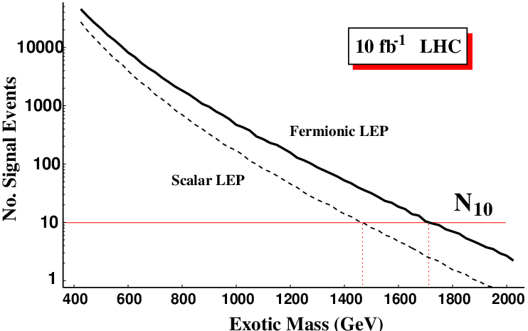

As the masses of the exotics increase, the production rate falls. We estimate the discovery reach in and via the muon signature channel in Figure 14. We use the standard practice of taking ten events to constitute the discovery threshold in cases with an exceptionally small number of expected background events. This corresponds to a mass reach of for the fermion and for the scalar exotic in 10 fb-1 of integrated luminosity. Since it should also be able to detect the fraction of events that stop somewhere in the detector itself, we also include the mass reach for this signature in Figure 15. Here the mass reach for 10 events is for the fermion and for the scalar. These rough estimates for the discovery reach of quasi-stable -charged objects are in good agreement with calculations performed in other model contexts Kraan:2005ji; Kilian:2004uj; Hewett:2004nw.
V Prompt Decay Signatures
Our intention is to study the presence of exotic supermultiplets in the presence of “standard” supersymmetric states such as those of the MSSM. This is motivated by a number of considerations. First, the study of the collider signatures of -inspired exotics in isolation has been performed by a number of authors. The signatures and analysis strategies for these cases are by now well understood. For example, a scalar state which decays directly into a lepton + quark or into two quarks can be reliably reconstructed by looking at the invariant mass distribution of leptons + jets and pairs of jets, respectively. This is possible even in the presence of Standard Model backgrounds and a measurement of the mass of the exotic scalar can readily be made Cakir:2005iw. It is therefore more interesting to consider the situation when a richer spectrum of “new physics” is present.
Second, most theoretical models of supersymmetric physics that have an ultraviolet completion – whether a GUT model or some sort of string construction – tend to predict that the exotics described in Section II will be present in conjunction with the states of the MSSM. In fact, as alluded to in the Introduction, they will typically arise with additional gauge fields (and their gaugino partners) and additional scalars. Therefore, considering the exotics in isolation may oversimplify the experimental challenges associated with these fields. Finally, it is interesting to ask how the presence of MSSM superpartners can serve as “background” to the identification, extraction and eventual study of exotic new supermultiplets – and indeed how the exotic states can complicate otherwise well-established analysis routines for supersymmetric parameter measurements.
In this section we will study the collider signatures of our exotic benchmark cases from Table 2. We will focus primarily on the leptoquark scenario for technical reasons, but we will occasionally address the diquark scenario as well. We reserve a full treatment of the diquark cases to a future publication. We allow the full set of interactions between exotics and MSSM states given in equations (2.3) or (2.4), but restrict ourselves to interactions between the exotic states and the first generation of Standard Model/MSSM states. We will also restrict the interactions with gauginos and Higgsinos to include only those states of the MSSM (i.e., we continue to neglect the possible presence of additional singlets or factors). This truncation reduces the model-dependence of the study considerably and corresponds to plausible limits of full-scale extended models Barger:2005hb; Barger:2006kt. We will also restrict attention to a single exotic fermion and the lighter exotic scalar, and will ignore the possibility of heavier generations of exotic particles. The latter would generally be expected to decay rapidly to the lightest generation if they mix and are sufficiently heavy, or else to exhibit production and decay patterns similar to to those of the lightest generation. Finally, we ignore decays into the right handed neutrino and its scalar partner. Depending on the model of neutrino mass generation, their masses might or might not be relevant at the LHC Kang:2004ix. If they are sufficiently light, the effects of the term in (2.3) would be similar to those from the neutrino part of the term.
V.1 Decays of Exotics
The majority of previous studies on the collider phenomenology of leptoquarks and diquarks have focused on non-supersymmetric scenarios in which the exotic state decays directly to Standard Model states. This may arise through mixing operators or by considering only the production and decay of scalar exotics with branching fractions to pairs of SM fermions set to unity Andre:2003wc; Mehdiyev:2006tz; Hewett:1987yg; Blumlein:1996qp; Dion:1997jw; Eboli:1997fb; Dion:1998wr. In order to discuss the full range of supersymmetric decays available – and to study the interesting issues outlined in the introduction to this section, it is necessary to postulate a fixed spectrum of MSSM states to include with the five scenarios of Table 2.
| Param. | SPS 1a | Param. | SPS 1a |
|---|---|---|---|
| 99.9 | 381.4 | ||
| 188.4 | 587.3 | ||
| 375.5 | , | 535.3 | |
| 394.0 | , | 554.5 | |
| 187.7 | 504.5 | ||
| 394.7 | 535.0 | ||
| 627.9 | , | 534.4 | |
| B-ino% | 97.4% | , | 559.3 |
| 111.7 | 145.5 | ||
| 412.7 | 220.6 | ||
| 420.3 | , | 145.8 | |
| 369.4 | , | 211.4 |
Our MSSM “background” sample corresponds to the minimal supergravity point SPS 1a, from the Snowmass Points & Slopes Allanach:2002nj. This point has a spectrum determined from the following set of minimal supergravity parameters: a unified scalar mass , a unified gaugino mass , a unified trilinear scalar coupling , and positive parameter. These soft supersymmetry-breaking values are specified at a high-energy input scale, here assumed to be the GUT scale (). These GUT-scale parameters are passed directly to PYTHIA, which then generates the physical mass spectrum for the MSSM at the electroweak scale. This process involves using approximate analytical solutions to the renormalization group equations (RGEs) for the soft Lagrangian parameters. Superpartner masses are computed at tree level, except for the Higgs sector which is computed from the full one-loop effective potential. The result is given in Table 4. A more careful treatment of the RGEs and/or the physical eigenstate masses might correct these numbers by as much as 10%, but the accuracy achieved here is sufficient for out purposes.
Snowmass Point 1a is the benchmark point from Allanach:2002nj most favorable for SUSY discovery at the LHC. It is therefore one of the most-studied supersymmetric models in the literature. All the superpartners are within reach of the LHC (and indeed, some may be detectable at the Tevatron with sufficient integrated luminosity). The relatively light scalar leptons are particularly important for this benchmark point, as they significantly enhance the event rate for trileptons and large missing transverse energy () through the production of electroweak gauginos. The relatively light gluino also ensures a large rate for multi-jet events with large . We will discuss these properties in the following subsections.

The five cases in Table 2 were selected to provide a range of possible decay chains between the exotic states, the MSSM spectrum and Standard Model states. The most important of the relevant mass scales are shown schematically in Figure 16. Mass differences between the exotic fermion and the lightest exotic scalar are given in terms of the variable introduced in (2.9) for the five cases (note that for cases A-C). Key thresholds are indicated by superpartner masses for the two lightest neutralinos , the gluino , the lightest first-generation sleptons and the lightest first-generation squarks . Note that the exotic fermion and its lightest scalar partner are each above 300 GeV in mass in all five cases.
In the first three cases of Table 2 the fermion is the lightest exotic particle (LEP). For the leptoquark scenario the two-body decay channels to a scalar lepton and a (massless) quark are always available due to the very low-mass sleptons in the SPS 1a model. Taking , the branching fractions for into the final states , and are 28%, 50% and 22%, respectively for cases A-C. For the diquark scenario the equivalent two-body decays to a quark and squark are kinematically forbidden. In this case the fermionic diquark must decay via three-body channels into states involving gauginos and two SM quarks. For our analysis we will only consider cases in which the final state involves the LSP neutralino. These three-body decay rates are given in Appendix B for decays via first-generation virtual squarks, as are those for the leptoquark case (relevant in different kinematic regimes for which the two-body decays are forbidden).
For both the leptoquark and diquark scenarios the direct decay into Standard Model fermions is the only channel kinematically available to the exotic scalar in Case A. The diquark has a single channel , while the leptoquark has two final states with relative branching fractions of 67% and 33%, respectively. For Case B the channel opens up, but the decays to fermion pairs continue to dominate. In the leptoquark case with the two SM channels sharing the remainder in the ratio of 2:1. For the diquark case for , with the other 95% accounted for by the two quark final state. For Case C all four neutralino final states are available, as is the decay process . This latter mode is the dominant channel, with a branching fraction of 87% in the leptoquark case and 77% in the diquark case. The next largest branching fraction for the leptoquark is and for the diquark is . The decay possibilities for the cases A-C are summarized in Table 5. As an example we give in Figure 17 the branching fraction into the seven allowed final states for decays of the scalar as a function of the size of the leptoquark Yukawa interaction. For convenience we here take . The vertical dotted line at defines the model we will consider in Section V.2.
| Case A | Case B | Case C | ||||
| Decay | ||||||
| partner + | ||||||
| partner + | ||||||
| partner + | ||||||
| partner + | ||||||
| partner + | ||||||
| NA | NA | NA | ||||
| NA | NA | NA | ||||

The scalar partner is the LEP for cases D and E. Here the scalar always decays via the Yukawa couplings of (2.3) and (2.4) to pairs of SM fermions. Case D was designed to allow the decays , as well as decays via the Yukawa interaction to final states. The branching fraction for decay into the exotic scalar + LSP is 32% for the leptoquark and 72% for the diquark. In the latter case, decays into final states are suppressed by the relatively large squark mass scale. Final states such as and are similarly suppressed for the leptoquark. In this latter case the final states , and each have branching fractions in the 20-24% range, making them competitive with the final state. The branching fraction for into the eight allowed final states are plotted in Figure 18 as a function of Yukawa coupling . Again we indicate the choice by the vertical dotted line. For Case E the very large mass difference between the fermion and scalar LEP allows all decay processes for both leptoquark and diquark. Here the dominant rate is to with branching fractions of 97% and 94%, respectively. The decay possibilities for cases D and E are summarized in Table 6.

| Case D | Case E | |||
| Decay | ||||
| partner + | ||||
| partner + | ||||
| partner + | ||||
| partner + | ||||
| partner + | ||||
| NA | NA | |||
| NA | NA | |||
Each individual decay channel was given its own position in unused entries in the BRAT and KFDP common blocks in PYTHIA. Two-body decays are computed at initialization by the new routine PYEXDC on the basis of user-designated Yukawa interactions and particle masses. Three-body decays require a more sophisticated treatment due to the numerical phase space integrations required. For these specific decays the result of these numerical integrations are given directly to PYTHIA for the five scenario points in Table 2.
V.2 Collider Signatures
We now turn our attention to the signature for these exotic supermultiplets at the CERN LHC. We are interested in what can be learned about the exotic component of the SUSY signal in the earliest stages of LHC data collection and analysis. Hence we will study 5 fb-1 of simulated signal data, where the signal here includes both the events associated with the SPS 1a benchmark point and one of our five exotic scenarios. Signatures involving the diquark tend to be multi-jet events with slightly less missing transverse energy than a “typical” MSSM SUSY event. As we will not be simulating Standard Model backgrounds for QCD jet events, making meaningful statements about signal-to-background estimations is difficult, even with a full detector simulation. A realistic study of such exotics would require a more sophisticated treatment of SM multi-jet backgrounds than we are providing in the current work. Furthermore, an additional technical difficulty arises in this case when hadronizing the out-going partons in PYTHIA when non-standard (i.e. non-planar) color flows are involved.1717 17 Unfortunately, we have yet to find an adequate solution to this problem, which (to the authors’ knowledge) afflicts all publicly-available event generation software. For these two reasons we will defer the treatment of the case of diquark couplings for the exotic multiplets to a subsequent publication, when the technical issues mentioned here can be more adequately resolved.
For the leptoquark scenario the Standard Model backgrounds are similar to those of typical SUSY events and have been studied elsewhere Baer:1995nq; Baer:1995va; Hinchliffe:1996iu. In this paper we will rely on those estimates to allow us to discuss the collider signatures without computing the relevant background samples. Nevertheless, a sample of 200,000 and 40,000 // events were generated for examining the efficiency of our cuts in isolating the exotic leptoquark signal from both the Standard Model and MSSM backgrounds. We proceed by simulating the events with PYTHIA and then pass the events to PGS PGS to simulate the detector response. The detector parameters are those of the hybrid ATLAS/CMS detector used by the LHC Olympics LHCO. As we do not wish to concern ourselves unduly with detailed issues of triggering, we have chosen to utilize the simplified triggering algorithm from version 3.0 of the PGS package. More specifically, we will analyze events for which the quantity , where
| (5.24) |
The objects appearing in the summation above are candidate objects; e.g. the electrons and muons in the first term in (5.24) are trigger-level electrons and muons. The taus in (5.24) are hadronically-decaying tau-candidates. Crudely speaking, electron and muon candidates must have , hadronically-decaying tau candidates and jet candidates must have and must be greater than 50 GeV to appear in the trigger function.
V.2.1 Can the new physics be definitively detected?
As mentioned in the previous subsection, the spectrum for Snowmass Point 1a gives rise to signatures that have been extensively studied in the past. The presence of excesses above Standard Model predictions can be definitively established in multiple channels in this scenario for even a handful of inverse femptobarns of integrated luminosity. The most important of these channels are multi-jet final states, multi-jets plus one or more leptons, events with same-sign pairs of leptons and any number of jets, trilepton events, and events with three taus in the final state Barnett:1987dj; Baer:1991xs; Kane:2002qp. All of these cases are for events accompanied by large values.
| Sample | Accepted Events | Percentage |
|---|---|---|
| SPS 1a | 185,544 | 93.1% |
| Case A | 161,284 | 85.0% |
| Case B | 156,020 | 84.7% |
| Case C | 152,342 | 84.5% |
| Case D | 11,589 | 96.8% |
| Case E | 17.921 | 94.0% |
We expect the additional contribution from the isosinglet exotics to add to these event rates – making the discovery of “new physics” even more rapid. In 5 fb-1 of integrated luminosity 185,544 MSSM events from SPS 1a passed our low-level trigger function (an acceptance rate of about 93%). The corresponding number of accepted events for the five exotic scenarios is given in Table 7. The relatively large production rate for the light exotic fermion in cases A-C nearly doubles the new physics sample, while the light-scalar scenarios provide only a small additional contribution. Not all of these additional events, however, will enter the SUSY search analyses.
Let us consider the bluntest, but most effective, tool for establishing the presence of beyond-the-Standard Model physics: the analysis for events with multiple high- jets and large Baer:1995nq. Following Hinchliffe:1996iu we select events with at least four jets, no isolated leptons with , transverse sphericity , and . We require the of the hardest jet to be at least 100 GeV and the of the four hardest jets to each be above 50 GeV. The variable is given by the scalar sum
| (5.25) |
where is the transverse momentum of the -th jet, ranked in order of value. We plot this quantity for the SPS 1a model together with each of the five exotic scenarios in Figure 19. For mass bins with a clear excess over the rapidly-falling Standard Model background should be visible.

Note, however, that the additional exotic component adds very little to the event sample in this analysis. While 33,836 events in the SPS 1a sample pass the above event selection cuts, less than 3,000 events pass them in cases A-C, while for cases D and E only 410 and 490 events, respectively, enter the analysis. Even if we allow events with any number of high- leptons we increase the SPS 1a acceptance by a factor of 1.5, but for the exotic samples the increase is only a modest factor of 3 for the fermion LEP cases and 2 for the scalar LEP cases. The most severe cuts turn out to be the requirement of four hard jets and the cut on . We prefer not to relax the cut without a thorough understanding of the Standard Model backgrounds. But in Figure 20 we plot the quantity for all objects in events with at least two jets, each with and any number of leptons (the other cuts remaining the same as before). The scalar LEP cases continue to contribute very little to the analysis, but now some structure is evident in the distribution for the fermionic LEP cases, albeit for low-energy bins where Standard Model processes will likely be dominant. In Figure 21 we focus on Case A where we show the individual contributions to the variable of Figure 20 from SPS 1a and from the fermionic LEP Case A. The two distributions are clearly separated, with the SPS 1a peak representing squark and gluino production while the peak for exotic Case A represents fermion LEP pair production. Whether or not the peak in this distribution at lower values is observable over the Standard Model background is an open question that will require further study with full background simulation.


As our exotic signal will generally involve one or more hard leptons in the final state we might expect that the inclusive signatures involving leptons will be more highly augmented over the SPS 1a case alone. In Figure 22 we give the event rate for the six key inclusive signatures studied in Baer:1995nq; Baer:1995va; Kane:2002qp for SPS 1a and the five exotic scenarios of Table 2. The first inclusive signature involves the event sample for the analysis: multi-jet events with large and no isolated leptons. The other five of these discovery modes involve high- leptons. They are jet events with single isolated leptons, events with jets and opposite-sign (OS) dileptons, events with jets and same-sign (SS) dileptons, events with three leptons and jets and events with three high- taus. All of these signatures involve large missing transverse energy.

In contrast to Ref. Kane:2002qp we give numbers of events of these signature topologies after applying a set of cuts designed to reduce the Standard Model background. These cuts are based on those of Refs. Baer:1995nq; Baer:1995va. All events in Figure 22 have and , except for the multi-jet category where we require . For the multi-jet case we require the three hardest jets to have . For the other five signatures we require for the hardest jet and for the second-hardest jet. All events are required to have a transverse sphericity of . For the multi-jet case we veto events with leptons having and . For the topologies involving leptons we instead require that the leptons (or taus) be isolated and have .
As expected, the multi-jet channel is overwhelmingly populated with events from the MSSM states. Event rates for the leptonic final states for cases A-C (with the fermion LEP) can be competitive with those of standard SUSY – particularly for the OS dilepton case where the large production cross-section for fermionic LEPs couples with the unit branching ratio for these states to quark + slepton. For cases D and E (with the scalar LEP) the exotic contribution to these inclusive signatures is a very small fraction of the total event rate. Nevertheless, in a world with only the supersymmetric exotic sector the scalar-LEP models are likely discoverable on their own in 5 fb-1 of data in the trilepton and jets + lepton channels (particularly if judicious cuts on the size of are made in these events). The fermionic LEP models give strong signals in all leptonic channels. When combined with the large rate from SPS 1A it is clear that robust “discovery” modes for new physics will be present across the board, even in the early stages of LHC running.
V.2.2 Can the exotic component be extracted?
Observation of the combined event rates in the six channels of Figure 22 should give clear evidence of new physics at the LHC, and should furthermore strongly suggest supersymmetry as the source of that new physics signal. Yet it is not immediately clear that the exotic component – above and beyond the spectrum of the MSSM – would be recognized merely from the inclusive signature counts. Taking into account the logarithmic scale in Figure 22 we note that the MSSM processes still dominate most of the inclusive signatures, particularly for exotic cases D and E. Nevertheless, the signal is clearly ‘‘lepton rich’’ relative to SPS 1a alone. Presumably an attempt to fit initial data to paradigms such as minimal supergravity would be unable to reproduce the large rate for multi-lepton events.1818 18 It would be an interesting exercise to attempt such a fit within the context of a suitably general MSSM framework, such as the “minimal reasonable model” of Brhlik and Kane Brhlik:1998gu. The first suggestion of beyond-the-MSSM physics may therefore arise from fits to the data which suggest extremely light slepton masses (say, below the bounds set by direct search limits) or anomalously large branching fractions of gauginos to leptonic final states.
One can find additional hints from the data itself. We have already seen that plotting the effective mass of all objects in events with at least 100 GeV of , at least two jets of and any number of leptons produces a structure indicating some subset of events are not arising from gluino and/or squark production. Yet these low effective-mass bins may not be visible above the Standard Model background when the cuts of Ref. Baer:1995nq are loosened. Indeed, the rough topology of events arising from pair production of leptoquark pairs is not unlike top quark events; cuts designed to reduce the rather large background at the LHC will therefore tend to reduce the exotic signal in these channels as well.

Nevertheless, some basic observations may suggest a leptoquark interpretation for at least some of the signal events. Those events arising from either fermionic or scalar leptoquarks distinguish themselves from those arising from the MSSM states of SPS 1a in three main ways: (1) lower jet multiplicities, (2) higher lepton multiplicities and (3) lower values of . In Figure 23 we plot the distribution of missing transverse energy in all events for each of our data samples. The standard MSSM processes give rise to a broad distribution which peaks at relatively large values. For example, requiring a cut of 100 GeV only eliminates 9% of the data sample (as opposed to 75% of our sample and 87% of our diboson sample). In contrast, the fermionic LEP cases give a much sharper peak at roughly half the value of the SPS 1a case. Nearly 50% of these events have . For the scalar LEP cases we have a sizable production of the scalar exotic, which decays directly to two Standard Model fermions with almost no missing energy. The long shallow tails are from the production and decay of the much heavier exotic fermion. Missing transverse energy in Standard Model events tends to peak at or below 50 GeV and fall rapidly. This suggests that at least for the fermionic LEP cases, the bimodal distribution in for the joint case of MSSM + exotics should indicate two sets of fields being produced, both with production cross-sections suggestive of strongly-interacting states, but with different mass scales and decay topologies.

In Figure 24 we give the typical number of leptons per event for the individual data samples. In each case the leptons are required to have at least 20 GeV of transverse momentum, but no other cuts are applied to the events. The exotic leptoquark samples clearly favor higher lepton multiplicities, but the characteristics of these leptons themselves (such as computed solely from leading leptons, or the distribution of the hardest lepton) do not differentiate between the SPS 1a events and the exotic events. The experimentalist investigating these events will find no peaks in the invariant mass distributions of various pairs of leptons. However, the events with multiple high- leptons tend to be those events with less . Consider, for example, exotic case A in conjunction with the SPS 1a model. In Figure 25 the scalar sum of values for all leptons in events with at least two isolated leptons is plotted versus the missing transverse energy in those events. It is clear from Figure 25 that there is some rough anti-correlation between the energy accounted for by leptons and the amount of energy carried away by LSPs. The feature visible along the horizontal axis in the figure (that is, for extremely small values of ) with extremely energetic leptons are events involving the pair production of scalar leptoquarks – which have a sizable event rate for the 367 GeV scalar mass of this benchmark point. The events in this part of the scatter plot also appear in the low bins in Figure 23 for case A. All of the events in Figure 25 have high- jets, yet no such anti-correlation or low feature is apparent in the analogous scatter plot involving jet values.

At this stage, if we were confronted with cases A-C we might conclude that in addition to squarks and gluinos (with a mass-scale of approximately 600-800 GeV) we are also producing a second class of states with a mass-scale of approximately 300-500 GeV. The overall rate for pair production of new states of this mass is consistent with those states being fermions which interact through the strong interaction. Events of this class occur with smaller amounts of than the squark/qluino events, and are associated with increased numbers of leptons and fewer jets. The association of strongly-coupled physics with prompt leptons and smaller but still significant signals may suggest a supersymmetric leptoquark interpretation. For cases D and E, where the event rates are lower, the signal is muted or non-existent and the Standard Model backgrounds are more problematic; it is unlikely that any deviation from the MSSM spectrum would be apparent given the crude observations presented here.
We have argued that 5 fb-1 of integrated luminosity is likely sufficient to reveal the presence of supersymmetric new physics. In the three cases involving a light exotic fermion it is also likely sufficient to reveal one or more objects with a production rate indicative of strong coupling but with decay chains in which high- leptons are prominent. Even in cases D and E for which there will be little evidence for an exotic component to the SUSY signal, it is still likely that experimental searches for leptoquarks will be performed nonetheless.

In Figure 26 we plot the invariant mass distribution of the hardest lepton and softest jet in events with precisely two jets and two (opposite-sign) leptons. Jets were required to have at least 50 GeV of transverse momentum and events were vetoed if either jet was B-tagged. A cut was made on the of the leading lepton of 50 GeV, and 20 GeV for the trailing lepton. Finally, we require the events to be somewhat collimated along the event axis, so we require the transverse sphericity to be no greater than 0.7. This final cut significantly reduced the contamination from both Standard Model processes and SPS 1a events (an acceptance rate of approximately 0.04% for each).
For cases A-C the invariant mass of the jet/lepton pair shows an end-point just below 200 GeV. This correctly measures the mass combination
| (5.26) |
via the on-shell cascade decay . For cases A-C this happens to be very near the mass difference between the fermionic LEP and the lightest neutralino. Mass peaks arising from the scalar pair production with can be reconstructed for all scenarios in which there is significant scalar production (case C had only 38 scalar events in 5 fb-1 of data). The true mass value for the lighter scalar is given over the corresponding peak in Figure 26. We note that if a cut on missing energy of were applied, the scalar mass peaks would vanish from the distributions in Figure 26, though the end-point in the distribution associated with fermion pair-production would still be visible.
These peaks can be isolated and sharpened by making stricter cuts on the data set, such as demanding , requiring the scalar sum of values from the two jets and two leptons sum to at least 400 GeV, and requiring the invariant mass of the lepton pair to be at least 100 GeV. An important cross-check is to find the same peak in the jet/lepton invariant mass distribution in associated production of scalar leptoquarks through the process . We can isolate this process by requiring (a) at least two jets without B-tags, the hardest jet having at least 200 GeV of transverse momentum and all others having , (b) precisely one isolated lepton with , and (c) . Pairing the second hardest jet with the single lepton gives a clear peak at the same mass values as those in Figure 26.
Thus, in every one of the scenarios of Table 2 there should be at least one exotic state, and occasionally two such states, which can be identified at the LHC – even with limited initial data. With additional statistics it should be possible to measure the masses of low-lying scalar mass eigenstates in all five scenarios. Reconstruction of cascade decays with additional integrated luminosity should also allow a determination of the exotic fermion mass in all five cases. We note, however, that the presence of the (supersymmetric) exotic states can complicate the analysis of the signal arising from MSSM states.
As the simplest example, we may consider the flavor-subtracted dilepton invariant mass distribution for OS-dilepton events in Snowmass point SPS 1a. For low-mass SUSY points such as this, even a small data sample is sufficient to establish a sharp “edge” in the weighted sum of distributions given by
| (5.27) |
The quantity in (5.27) for SPS 1a is given by the dashed line in Figure 27. The edge at is the result of the flavor-subtraction procedure. When the pair of opposite-sign leptons arise from a single decay chain of , the two leptons are forced to be of the same flavor. When the two leptons come from two independent decays (as in the case of production, or pair production of squarks and gluinos) the probabilities for same-flavor and opposite-flavor lepton pairs are roughly the same. The subtraction procedure therefore efficiently isolates the exclusive decay chain for decays and produces a sharp edge at the value
| (5.28) |
which happens to be very nearly the mass difference in Snowmass point 1a.

Yet the effectiveness of this subtraction procedure is a result of the flavor-democracy of Standard Model gauge interactions (which are related to the decay rates of gauginos by supersymmetry). For our exotic states these decays are governed by Yukawa interactions which (up to model-dependent constraints from flavor-changing processes discussed in Section III.2) are largely free parameters. When the fermion LEP preferentially decays to one flavor of lepton, for example, the subtraction technique will fail to completely isolate gaugino decays. We show this effect by the solid line in Figure 27 where Snowmass point SPS 1a is analyzed together with the exotic states of Case A. In this case the exotic is decaying exclusively to first-generation leptons. The distribution still exhibits an edge (suggesting on-shell sleptons in the decay chain), but the significance to this shape fitting will diminish greatly without changes to the manner in which the gaugino signal is extracted. This will necessarily degrade the accuracy with which mass differences between low-lying superpartners and the LSP can be determined.
VI Conclusions
In this work we have provided a case study on how “New Physics” might appear in the early stages of the LHC experiment at CERN. If this new physics is the minimal supersymmetric standard model (or even more specifically, one of the specially-defined benchmark points of this model that have been designed by theorists), then it is very likely that the presence of the new physics and measurement of many key properties will be straightforward. It is not at all unlikely, however, that a supersymmetric world may be far from minimal. Evidence in support of this comes both from top-down constructions of GUT or string models as well as considerations of a bottom-up nature which focus on naturalness of the electroweak symmetry-breaking sector in SUSY Dine:2007xi; Brignole:2003cm; Casas:2003jx.
We have presented here just such an alternative world that is very much a plausible outcome of semi-realistic string constructions. The common element of these models is the presence of -charged squarks and quarks which are isosinglets under weak and carry equal and opposite hypercharge. Such states may present themselves as new ‘partners’ of Standard Model down-type quarks and squarks, as leptoquarks or diquarks, or may have more exotic properties which forbid renormalizable-level couplings altogether. We have used the language of to characterize these states for convenience, but GUT models are by no means the only way in which such states can arise. The potential phenomenology of these states is both rich and tightly constrained, providing an interesting scenario for untangling high-scale physics from the low-energy observables of the LHC.
If such states exist at LHC-accessible energies their presence will most surely be detected. This was the conclusion of previous work that considered such states in isolation, with only Standard Model fields serving as ‘background.’ In our work we have provided the first analysis of such fields in the simultaneous presence of ‘standard’ superpartners, using the benchmark point of SPS 1a as our example of simple SUSY models. The result of our study has been to point out important consequences for experimenters hoping to observe and measure the properties of new physics in both sectors. A strong supersymmetric signal will not be obscured by these exotic states, but recognition of the new states may not be immediate. In the interim, we can expect fits to standard SUSY-breaking paradigms such as minimal supergravity, to fit well initially. As the LHC experiments integrate luminosity, we expect statistically significant deviations from the predictions of the pure MSSM to arise. In the leptoquark exotic case considered here that deviation will first appear in events with both leptons and high- jets, but with little missing transverse energy. We anticipate that astute experimentalists will consider a leptoquark interpretation of these ‘anomalous’ events, but most SUSY analysis techniques (particularly those which seek to isolate certain cascade decay chains and therefore measure certain mass differences) will need significant refinement. We hope that the work presented here will spur others to provide a more sophisticated treatment of the quite-plausible ‘what-if’ scenario we provide, and to provide similar checks on the robustness of long-established analysis techniques.
Acknowledgements.
It is a pleasure to thank J. Erler for useful discussions. This work was supported by the U.S. Department of Energy under Grant No. DOE-EY-76-02-3071, by National Science Foundation Grants PHY99-07949 and PHY-0503584, and by the Friends of the IAS.Appendix A Alternative quasi-stable model
As mentioned in Section II.2, stability on the time-scale of the detector at a hadron collider can be accomplished by forbidding dimension-four operators that couple the exotic representations to the Standard Model. In Sections II.2 and III.3 this was illustrated by an -motivated model in which the dimension-four operators were forbidden by a combination of , , and symmetries. Here, we consider a toy model, which was first constructed in Erler:2000wu, in which this is achieved through a new gauge symmetry alone. We will impose charge assignments such that our exotics are stable at the renormalizable level but are allowed to decay through higher-dimensional operators. To achieve this we introduce an anomaly-free with chiral matter representations which include two representations of and various fields which will be singlets under the Standard Model (SM) gauge group. Since and are not imposed, we allow for the additional constraints imposed by the non-observation of proton decay.
| Field | Field | ||||
| 1/6 | 1 | 1/2 | -2 | ||
| -2/3 | 1 | -1/2 | -2 | ||
| 1/3 | 1 | -1/3 | -3 | ||
| -1/2 | 1 | 1/3 | -3 | ||
| 1 | 1 | -1/2 | -2 | ||
| 0 | 1 | 1/2 | -2 | ||
| 0 | 4 | 0 | 6 |
The field content of the model is given in Table 8. The charge assignments are obtained by solving the anomaly cancellation equations. For the charges listed below all the mixed anomalies of and vanish. Since we only include additional representations , we will not modify the SM gauge anomaly cancelations. However, additional SM singlets are still needed to cancel the trace anomaly and the anomaly. There is some freedom in choosing their charge assignments Erler:2000wu. Note that the model maintains the unification of the SM gauge couplings at one loop. In fact, complete unification can be achieved for the appropriate rescaling of the gauge coupling . However, there is no simple explanation of the charge quantization, analogous to the charge quantization in ordinary grand unification theories, since the charge assignments are just numerical solutions to the anomaly cancelation equations.
Aside from the usual Yukawa interactions of the MSSM, the superpotential terms allowed by the choice of charges in Table 8 are given by
| (A.1) | |||||
| (A.2) | |||||
The exotic particles and are stable at renormalizable level: there is only one operator involving that is allowed by the symmetry, and one can therefore assign a conserved number. This operator can provide a mass term for the exotic quarks should a -breaking vacuum expectation value develop. The and doublets can decay by the dimension 4 operators.
There are a number of -number violating interactions allowed at dimension 5, however. These operators also violate baryon and lepton numbers, leading to proton decay. The operators can be divided into two sets. The first two rows of (A.2) would allow conservation for the assignment for , while the last row of (A.2) would require . Clearly, if operators from both sets are present will be violated and the proton will decay. However, since the -number is conserved at dimension-4 level (and the is assumed to be heavier than the proton), the proton decay rate is proportional to , where is the scale multiplying the dimension-5 operators. Depending on which operators are included, the dominant decay processes are () or (), or the corresponding neutron decays .1919 19 Decays into are highly suppressed because the operator must be antisymmetric in the flavor indices, leading to decays including a virtual or quark. The experimental limits for these processes are and Eidelman:2004wy. If the operator is present, with the scalar components of and acquiring VEVs, as well as or , the proton decay constraint is satisfied provided that . Alternatively, if is replaced by , then is sufficient.
Appendix B Explicit Cross-Section and Partial Width Expressions
In keeping with the conventions of PYTHIA we quote parton-level cross sections for processes as differential cross-sections of the form . In what follows the kinematic factor is given by
| (B.1) | |||||
where the last relation holds when . We will also have occasion to use the quantity
| (B.2) |
In PYTHIA the parton-level Mandelstam variables are given by
| (B.3) |
where is the polar angle of parton 3 in the c.m. frame of the hard scattering.
B.1 Production Cross Sections
- •
There are two parton-level sub-processes of relevance: the - annihilation (two quarks of the same flavor) through gluon exchange in the direct channel and a diagram with t-channel exchange of a squark or slepton through the Yukawa interaction. The differential cross-section for the leptoquark case is given by
(B.4) where . For the diquark case we have
(B.5) Note the following: (1) In doing the PYTHIA analysis we always take , and . So expressions involving should be understood as involving the common value of this Yukawa interaction. (2) For the Snowmass point we use as our superpartner spectrum, the up and down type left-handed squarks have the same masses to within a percent and up and down right-handed squarks have the same masses to within less than a percent. Thus, in evaluating (B.5) PYTHIA takes just the (common) soft mass and soft masses.
- •
There are two sub-diagrams for this process: the diagram with the initial gluons leading to a gluon intermediate state and then to two fermions, and the t-channel/u-channel exchange of the heavy fermion . The differential cross-section is given by
(B.6) plus the equivalent expression with .
- •
For this process there are two types of diagrams: - annihilation (two quarks of the same flavor) through gluon exchange in the direct channel and t-channel exchange of a Standard Model fermion. As we allow our exotics to interact solely with first generation Standard Model fermions, the appropriate differential cross-section is
(B.7) when , are a flavor other than the first generation and
for first-generation ,.
- •
The QCD diagrams for the diquarks and leptoquarks are the same. There are several sub-diagrams: the diagram with the initial gluons leading to a gluon intermediate state and then to two scalars, the t-channel/u-channel exchange of the heavy scalar , and the “sea-gull” four-point diagram. The appropriate differential cross-section is given by
(B.8) - •
Single scalar leptoquarks and diquarks can be produced in association with a lepton and quark, respectively. The diagram involves initial states, either a quark in the direct channel or an exotic squark in the indirect (u) channel, and then a scalar and fermion in the final state. One of the two vertices is then given by QCD while the other is from the appropriate Yukawa coupling. The expression for the leptoquark is given by
(B.9) The equivalent expression for the diquark gets an extra factor of two from the different color contraction.
- •
This case is slightly different. What’s coded into PYTHIA is , and this is given in turn by
(B.10)
B.2 Two-Body Decays
For two-body decays of the form let us define the final momentum in the rest frame of as
| (B.11) |
Furthermore, we define the exotic scalar mixing matrix by the relations
| (B.12) |
Then the partial widths for the exotic decay channels considered are given by the following:2020 20 We always give the spin-averaged decay rate for the exotic fermions. For QCD production, this ignores spin correlations between the produced and . It also neglects possible polarizations for leptoquark or diquark production processes.
- •
(B.13) where the is from color.
- •
(B.14) where , , and is the mixing element relating to the bino (wino). We ignore contributions to decays from neutralinos associated with the Standard Model singlet (singlinos) or additional (-gauginos).
- •
(B.15) - •
(B.16)
- •
For the process , neglecting fermion masses and taking and , we have
(B.17) with
(B.18) - •
When kinematically allowed, the rate for the process is given in the same approximation above by
(B.19) with for all decays and , for decays to left-handed and right-handed squarks, respectively.
B.3 Three-Body Decays
Finally, we give the rates for three-body decays. Let us keep only the first generation of Standard Model fermions and ignore mixing, except for the exotic scalars whose mixing is defined in (B.12). We continue to ignore contributions to decays from singlinos or -gauginos. We will also ignore Higgsino contributions. We define the quantities
| (B.20) |
| (B.21) |
| (B.22) |
| (B.23) |
| (B.24) |
| (B.25) |
| (B.26) |
where and are the entries of the () neutralino mass matrix. In practice we will take and .
Let us begin by considering the process via the operator with coefficient in (2.4). Diagrams leading to this final state can involve the virtual state or virtual right-handed squarks. The amplitude-squared, summed over final colors and averaged over initial spins, is given by
| (B.27) |
where is the color factor for this process and
| (B.28) | |||||
The are given by the expressions
| (B.29) |
| (B.30) |
All outgoing momenta are assumed to be physical momenta. In the rest frame of the initial state we therefore have the products
| (B.31) |
| (B.32) |
| (B.33) |
| (B.34) |
| (B.35) |
| (B.36) |
The decay rate can be computed by integrating the partial width
| (B.37) |
where . The numerical integration can be performed for (but retaining ) by following standard techniques Barger.
For massless quarks, there is no interference between the diagrams involving the vertex and those from the vertex. The latter may be obtained from the above by the substitutions
| (B.38) |
Thus, for example, we have
| (B.39) |
where
| (B.40) |
| (B.41) |
| (B.42) |
| (B.43) | |||||
For leptoquark processes we distinguish between rates to and final states. In analogy to the and factors above, we define the quantities
| (B.44) |
| (B.45) |
| (B.46) |
| (B.47) |
| (B.48) |
| (B.49) |
The appropriate three-body decay rates can then be found following the above description using the substitution rules summarized in Table 9
References
- (1) P. Binetruy, G. L. Kane, B. D. Nelson, L. T. Wang and T. T. Wang, Phys. Rev. D 70, 095006 (2004).
- (2) B. C. Allanach, D. Grellscheid and F. Quevedo, JHEP 0407, 069 (2004).
- (3) A. Datta, G. L. Kane and M. Toharia, “Is it SUSY?,” arXiv:hep-ph/0510204.
- (4) B. C. Allanach and C. G. Lester, Phys. Rev. D 73, 015013 (2006).
- (5) N. Arkani-Hamed, G. L. Kane, J. Thaler and L. T. Wang, JHEP 0608, 070 (2006).
- (6) T. Plehn, Czech. J. Phys. 55, B213 (2005).
- (7) P. Langacker, Phys. Rept. 72, 185 (1981).
- (8) J. L. Hewett and T. G. Rizzo, Phys. Rept. 183, 193 (1989).
- (9) M. Cvetic and P. Langacker, Phys. Rev. D 54, 3570 (1996).
- (10) M. Cvetic, D. A. Demir, J. R. Espinosa, L. L. Everett and P. Langacker, Phys. Rev. D 56, 2861 (1997) [Erratum-ibid. D 58, 119905 (1998)].
- (11) E. Keith and E. Ma, Phys. Rev. D 56, 7155 (1997).
- (12) P. Langacker and J. Wang, Phys. Rev. D 58, 115010 (1998).
- (13) Y. Daikoku and D. Suematsu, Phys. Rev. D 62, 095006 (2000).
- (14) J. Erler, Nucl. Phys. B 586, 73 (2000).
- (15) J. R. Ellis, J. F. Gunion, H. E. Haber, L. Roszkowski, and F. Zwirner, Phys. Rev. D39, 844 (1989).
- (16) I. Antoniadis, C. P. Bachas and C. Kounnas, Nucl. Phys. B 289, 87 (1987).
- (17) H. Kawai, D. C. Lewellen and S. H. H. Tye, Phys. Rev. Lett. 57, 1832 (1986) [Erratum-ibid. 58, 429 (1987)].
- (18) H. Kawai, D. C. Lewellen and S. H. H. Tye, Phys. Rev. D 34, 3794 (1986).
- (19) I. Antoniadis, J. R. Ellis, J. S. Hagelin and D. V. Nanopoulos, Phys. Lett. B 231, 65 (1989).
- (20) A. E. Faraggi, Phys. Lett. B 326, 62 (1994).
- (21) S. Chaudhuri, S. W. Chung, G. Hockney and J. D. Lykken, Nucl. Phys. B 456, 89 (1995).
- (22) G. Cleaver, M. Cvetic, J. R. Espinosa, L. L. Everett, P. Langacker and J. Wang, Phys. Rev. D 59, 055005 (1999).
- (23) G. B. Cleaver, A. E. Faraggi and D. V. Nanopoulos, Int. J. Mod. Phys. A 16, 425 (2001).
- (24) J. Giedt, Annals Phys. 297, 67 (2002).
- (25) C. Panagiotakopoulos and K. Tamvakis, Phys. Lett. B469, 145 (1999).
- (26) C. Panagiotakopoulos and A. Pilaftsis, Phys. Rev. D63, 055003 (2001).
- (27) A. Menon, D. E. Morrissey, and C. E. M. Wagner, Phys. Rev. D70, 035005 (2004).
- (28) R. Dermisek and J. F. Gunion, Phys. Rev. Lett. 95, 041801 (2005).
- (29) U. Ellwanger, J. F. Gunion and C. Hugonie, JHEP 0507, 041 (2005).
- (30) V. Barger, P. Langacker, H. S. Lee and G. Shaughnessy, Phys. Rev. D 73, 115010 (2006).
- (31) D. O’Connell, M. J. Ramsey-Musolf, and M. B. Wise, Phys. Rev. D 75, 037701 (2007).
- (32) V. Barger, P. Langacker and G. Shaughnessy, Phys. Rev. D 75, 055013 (2007).
- (33) R. Dermisek and J. F. Gunion, arXiv:0705.4387 [hep-ph].
- (34) V. Barger, P. Langacker, M. McCaskey, M. J. Ramsey-Musolf and G. Shaughnessy, arXiv:0706.4311 [hep-ph].
- (35) For a review, see V. Barger, P. Langacker and G. Shaughnessy, arXiv:hep-ph/0702001.
- (36) M. L. Perl, P. C. Kim, V. Halyo, E. R. Lee, I. T. Lee, D. Loomba and K. S. Lackner, Int. J. Mod. Phys. A 16, 2137 (2001).
- (37) G. F. Giudice, E. W. Kolb and A. Riotto, Phys. Rev. D 64, 023508 (2001).
- (38) A. Kudo and M. Yamaguchi, Phys. Lett. B 516, 151 (2001).
- (39) J. R. Ellis, K. Enqvist, D. V. Nanopoulos and F. Zwirner, Nucl. Phys. B 276, 14 (1986).
- (40) F. Zwirner, Int. J. Mod. Phys. A 3, 49 (1988).
- (41) R. R. Volkas, A. J. Davies and G. C. Joshi, Phys. Rev. D 38, 311 (1988).
- (42) D. Suematsu, Prog. Theor. Phys. 96, 611 (1996).
- (43) J. Erler, P. Langacker and T. j. Li, Phys. Rev. D 66, 015002 (2002).
- (44) A. V. Kartavtsev, Nucl. Part. Phys. 31, 1191 (2005).
- (45) J. Kang and P. Langacker, Phys. Rev. D 71, 035014 (2005).
- (46) J. Kang, P. Langacker and T. Li, Phys. Rev. D 71, 015012 (2005).
- (47) S. F. King, S. Moretti and R. Nevzorov, Phys. Rev. D 73, 035009 (2006); Phys. Lett. B 634, 278 (2006).
- (48) E. Witten, Nucl. Phys. B 258, 75 (1985).
- (49) M. K. Gaillard and R. l. Xiu, Phys. Lett. B 296, 71 (1992).
- (50) S. P. Martin and P. Ramond, Phys. Rev. D 51, 6515 (1995).
- (51) T. G. Rizzo, Phys. Rev. D 46, 5102 (1992).
- (52) E. Ma, Phys. Lett. B 380, 286 (1996).
- (53) V. D. Barger, N. Deshpande, R. J. N. Phillips and K. Whisnant, Phys. Rev. D 33, 1912 (1986) [Erratum-ibid. D 35, 1741 (1987)].
- (54) P. Langacker and D. London, Phys. Rev. D 38, 886 (1988).
- (55) T. C. Andre and J. L. Rosner, Phys. Rev. D 69, 035009 (2004).
- (56) R. Mehdiyev, S. Sultansoy, G. Unel and M. Yilmaz, Eur. Phys. J. C 49, 613 (2007).
- (57) J. L. Hewett and S. Pakvasa, Phys. Rev. D 37, 3165 (1988).
- (58) J. Blumlein, E. Boos and A. Kryukov, Z. Phys. C 76, 137 (1997).
- (59) B. Dion, L. Marleau, G. Simon and M. de Montigny, Eur. Phys. J. C 2, 497 (1998).
- (60) O. J. P. Eboli, R. Zukanovich Funchal and T. L. Lungov, Phys. Rev. D 57, 1715 (1998).
- (61) B. Dion, L. Marleau and G. Simon, Phys. Rev. D 59, 015001 (1999).
- (62) A. Pukhov et al., “CompHEP: A package for evaluation of Feynman diagrams and integration over multi-particle phase space. User’s manual for version 33,” [arXiv:hep-ph/9908288].
- (63) T. Sjostrand, L. Lonnblad, S. Mrenna and P. Skands, “PYTHIA 6.3: Physics and manual,” [arXiv:hep-ph/0308153].
- (64) T. Sjostrand and P. Z. Skands, Nucl. Phys. B 659, 243 (2003).
- (65) S. Atag, O. Cakir and S. Sultansoy, Phys. Rev. D 59, 015008 (1999).
- (66) O. Cakir and M. Sahin, Phys. Rev. D 72, 115011 (2005).
- (67) B. C. Allanach et al., Eur. Phys. J. C 25, 113 (2002) [eConf C010630, P125 (2001)].
- (68) R. M. Harris [CDF Collaboration], AIP Conf. Proc. 357, 72 (1996), arXiv:hep-ex/9506008.
- (69) F. Abe et al. [CDF Collaboration], Phys. Rev. Lett. 74, 3538 (1995).
- (70) F. Abe et al. [CDF Collaboration], Phys. Rev. D 55, 5263 (1997).
- (71) B. Abbott et al. [D0 Collaboration], Phys. Rev. Lett. 80, 2051 (1998).
- (72) B. Abbott et al. [D0 Collaboration], Phys. Rev. Lett. 84, 2088 (2000).
- (73) V. M. Abazov et al. [D0 Collaboration], Phys. Rev. Lett. 88, 191801 (2002).
- (74) V. M. Abazovet al. [D0 Collaboration], Phys. Lett. B 640, 230 (2006).
- (75) V. M. Abazov et al. [D0 Collaboration], Phys. Rev. D 71, 071104 (2005).
- (76) V. M. Abazov et al. [D0 Collaboration], Phys. Lett. B 636, 183 (2006).
- (77) V. M. Abazov et al. [D0 Collaboration], arXiv:0705.0812 [hep-ex].
- (78) D. Acosta et al. [CDF Collaboration], Phys. Rev. D 72, 051107 (2005).
- (79) A. Abulencia et al. [CDF Collaboration], Phys. Rev. D 73, 051102 (2006).
- (80) V. M. Abazov et al. [D0 Collaboration], Phys. Lett. B 647, 74 (2007).
- (81) S. Chekanov et al. [ZEUS Collaboration], Phys. Rev. D 68, 052004 (2003).
- (82) A. Aktas et al. [H1 Collaboration], Phys. Lett. B 629, 9 (2005).
- (83) D. Acosta et al. [CDF Collaboration], Phys. Rev. Lett. 90, 131801 (2003).
- (84) A. Heister et al. [ALEPH Collaboration], Eur. Phys. J. C 31, 327 (2003).
- (85) M. Chemtob, Prog. Part. Nucl. Phys. 54, 71 (2005).
- (86) R. Barbier et al., Phys. Rept. 420, 1 (2005).
- (87) V. D. Barger, G. F. Giudice and T. Han, Phys. Rev. D 40, 2987 (1989).
- (88) S. Davidson, D. C. Bailey and B. A. Campbell, Z. Phys. C 61, 613 (1994).
- (89) D. Choudhury and P. Roy, Phys. Lett. B 378, 153 (1996).
- (90) B. Allanach et al. [R parity Working Group Collaboration], “Searching for R-parity violation at Run-II of the Tevatron,” arXiv:hep-ph/9906224.
- (91) B. C. Allanach, A. Dedes and H. K. Dreiner, Phys. Rev. D 60, 075014 (1999).
- (92) B. A. Campbell, J. R. Ellis, K. Enqvist, M. K. Gaillard and D. V. Nanopoulos, Int. J. Mod. Phys. A 2, 831 (1987).
- (93) D. A. Morris, Phys. Rev. D 37, 2012 (1988).
- (94) G. D’Ambrosio and D. N. Gao, Phys. Lett. B 513, 123 (2001).
- (95) C. Dohmen et al. [SINDRUM II Collaboration.], Phys. Lett. B 317, 631 (1993).
- (96) J. E. Kim, P. Ko and D. G. Lee, Phys. Rev. D 56, 100 (1997).
- (97) K. Huitu, J. Maalampi, M. Raidal and A. Santamaria, Phys. Lett. B 430, 355 (1998).
- (98) R. Barbieri and A. Masiero, Nucl. Phys. B 267, 679 (1986).
- (99) C. E. Carlson, P. Roy and M. Sher, Phys. Lett. B 357, 99 (1995).
- (100) B. de Carlos and P. L. White, Phys. Rev. D 55, 4222 (1997).
- (101) P. Slavich, Nucl. Phys. B 595, 33 (2001).
- (102) G. Bhattacharyya and A. Raychaudhuri, Phys. Rev. D 57, 3837 (1998).
- (103) D. N. Spergel et al., Astrophys. J. Suppl. 170, 377 (2007).
- (104) M. Kawasaki, K. Kohri and T. Moroi, Phys. Lett. B 625, 7 (2005).
- (105) M. Kawasaki, K. Kohri and T. Moroi, Phys. Rev. D 71, 083502 (2005).
- (106) Y. I. Izotov and T. X. Thuan, Astrophys. J. 602, 200 (2004).
- (107) B. D. Fields and K. A. Olive, Astrophys. J. 506, 177 (1998).
- (108) J. K. Webb, R. F. Carswell, K. M. Lanzetta, R. Ferlet, M. Lemoine, A. Vidal-Madjar and D. V. Bowen, Nature 388, 250 (1997).
- (109) G. Jungman, M. Kamionkowski and K. Griest, Phys. Rept. 267, 195 (1996).
- (110) V. Barger and R. Phillips, Collider Physics, Addison Wesley, 1996.
- (111) A. Arvanitaki, C. Davis, P. W. Graham, A. Pierce and J. G. Wacker, Phys. Rev. D 72, 075011 (2005).
- (112) H. Baer, K. m. Cheung and J. F. Gunion, Phys. Rev. D 59, 075002 (1999).
- (113) A. Mafi and S. Raby, Phys. Rev. D 62, 035003 (2000).
- (114) A. C. Kraan, Eur. Phys. J. C 37, 91 (2004).
- (115) A. C. Kraan, J. B. Hansen and P. Nevski, Eur. Phys. J. C 49, 623 (2007).
- (116) W. Kilian, T. Plehn, P. Richardson and E. Schmidt, Eur. Phys. J. C 39, 229 (2005).
- (117) J. L. Hewett, B. Lillie, M. Masip and T. G. Rizzo, JHEP 0409, 070 (2004).
- (118)
Atlas Detector and Physics Performance: Technical Design
Report, ATLAS Collaboration, CERN-LHCC-99-14.
P. Paolucci, The CMS Muon System, CMS Conference Report, CMS NOTE 2006/006. - (119) A. Nisati, S. Petrarca and G. Salvini, Mod. Phys. Lett. A 12, 2213 (1997).
- (120) A. Arvanitaki, S. Dimopoulos, A. Pierce, S. Rajendran and J. G. Wacker, “Stopping gluinos,” arXiv:hep-ph/0506242.
- (121) V. Barger, P. Langacker and H. S. Lee, Phys. Lett. B 630, 85 (2005).
- (122) V. Barger, P. Langacker and G. Shaughnessy, Phys. Lett. B 644, 361 (2007).
- (123) H. Baer, C. h. Chen, F. Paige and X. Tata, Phys. Rev. D 52, 2746 (1995).
- (124) H. Baer, C. h. Chen, F. Paige and X. Tata, Phys. Rev. D 53, 6241 (1996).
- (125) I. Hinchliffe, F. E. Paige, M. D. Shapiro, J. Soderqvist and W. Yao, Phys. Rev. D 55, 5520 (1997).
- (126) http://www.physics.ucdavis.edu/ c̃onway/research/software/pgs/pgs4-general.htm
- (127) http://www.jthaler.net/olympicswiki/
- (128) R. M. Barnett, J. F. Gunion and H. E. Haber, Phys. Rev. Lett. 60, 401 (1988).
- (129) H. Baer, X. Tata and J. Woodside, Phys. Rev. D 45, 142 (1992).
- (130) G. L. Kane, J. D. Lykken, S. Mrenna, B. D. Nelson, L. T. Wang and T. T. Wang, Phys. Rev. D 67, 045008 (2003).
- (131) M. Brhlik and G. L. Kane, Phys. Lett. B 437, 331 (1998).
- (132) R. M. Barnett, J. F. Gunion and H. E. Haber, Phys. Lett. B 315, 349 (1993).
- (133) D. Denegri, W. Majerotto and L. Rurua, Phys. Rev. D 58, 095010 (1998).
- (134) M. M. Nojiri and Y. Yamada, Phys. Rev. D 60, 015006 (1999).
- (135) B. K. Gjelsten, D. J. Miller and P. Osland, JHEP 0412, 003 (2004).
- (136) B. K. Gjelsten, D. J. Miller and P. Osland, JHEP 0506, 015 (2005).
- (137) W. M. Yao et al. [Particle Data Group], J. Phys. G 33, 1 (2006).
- (138) M. Dine, N. Seiberg and S. Thomas, “Higgs Physics as a Window Beyond the MSSM (BMSSM),” arXiv:0707.0005 [hep-ph].
- (139) A. Brignole, J. A. Casas, J. R. Espinosa and I. Navarro, Nucl. Phys. B 666, 105 (2003).
- (140) J. A. Casas, J. R. Espinosa and I. Hidalgo, JHEP 0401, 008 (2004).