Unquenching Effects on the Coefficients of the Lüscher-Weisz Action

Recent progress in parallel computing, as well as theoretical advances in the formulation of lattice gauge theories with fermions, have allowed the widespread adoption of simulations using dynamical light quarks, leading to a significant reduction in systematic errors by removing the uncontrollable error inherent in the quenched approximation.

The Fermilab Lattice, MILC and HPQCD collaborations have an ambitious program which to date has made several high-precision predictions from unquenched lattice QCD simulations [1, 2]. In this, we rely on the Symanzik-improved staggered-quark formalism, specifically the use of the asqtad [3] action. While this approach requires the use of the fourth root of the staggered quark determinant, all the available evidence is consistent with the conclusion that the resulting theory is in the same universality class as continuum QCD, as long as the chiral limit is taken after the continuum limit [4].

Recent studies of the heavy-quark potential in full QCD [5] have shown an unexpected apparent increase in scaling violations compared to the quenched approximation. A possible reason for this would be that these scaling violations arise from the mismatch between the inclusion of sea quark effects in the simulation and the omission of sea quark effects in the improvement coefficients in the action. This mismatch would appear to spoil the $\mathcal{O}(a^{2})$ improvement at the level of $\mathcal{O}(\alpha_{s}N_{f}a^{2})$. While a systematic study of $\mathcal{O}(\alpha_{s}a^{2})$ effects is generally beyond the scope of the current perturbative improvement programme, it is still important to bring up-to-date the calculations of the Lüscher-Weisz improved gluonic action [6, 7] to include the effects of dynamical quarks. This is important also because the Lüscher-Weisz improvement is currently included in many unquenched simulations [3]. Since the lattice spacing scale is set by measurement of the heavy-quark potential, there will be an induced $\mathcal{O}(\alpha_{s}N_{f}a^{2})$ artifact by omitting the corrections due to unquenching. While such errors are generally smaller than other systematic errors in current state-of-the art studies, it is simple to remove them using the result of the perturbative matching calculations outlined here. For details, the reader is referred to our paper [8].

The Lüscher-Weisz action is given by [9]

where $P$, $R$ and $T$ are the plaquette, rectangle and “twisted” parallelogram loops, respectively. The requirement of obtaining the Yang-Mills action in the continuum limit imposes the constraint

which fixes $c_{0}$ given the other two coefficients. This leaves us with $c_{1}$ and $c_{2}$ to be determined in order to eliminate the $\mathcal{O}(a^{2})$ lattice artifacts.

If we have two independent quantities $Q_{1}$ and $Q_{2}$ which, at each order in perturbation theory, can be expanded in powers of $(\mu a)$, where $\mu$ is some energy scale, as

then the $\mathcal{O}(a^{2})$ matching condition reads

Since this equation is linear, we can decompose the $w_{i}$ into a gluonic and a fermionic part as $w_{i}=w_{i}^{\textrm{glue}}+N_{f}w_{i}^{\textrm{quark}}$ and obtain the same decomposition for the $c_{i}$; thus, especially we do not need to repeat the quenched calculation in order to obtain the $\mathcal{O}(N_{f})$ contributions.¹¹ 1 Although doing so provides a useful check on our methods, and we have in fact successfully reproduced the results of [7].

At tree-level, there are no fermion loops to consider, and hence the tree-level coefficients remain unchanged compared to the quenched case [6]:

In lattice perturbation theory, the link variables $U_{\mu}\in SU(N)$ are expressed in terms of the gauge field $A_{\mu}\in su(N)$ as

which, when expanded in powers of $g$, leads to a perturbative expansion of the lattice action, from which the perturbative vertex functions can be read off.

As in any perturbative formulation of a gauge theory, gauge fixing and ghost terms appear in the Fadeev-Popov Lagrangian; an additional term arises from the Haar measure on the gauge group. Here we will not have to concern ourselves with these, since for our purpose we only need to consider quark loops.

To handle the complicated form of the vertices and propagators in lattice perturbation theory, we employ a number of automation methods [11, 12] that are based on the seminal work of Lüscher and Weisz [6]. Three independent implementations by different authors have been used in this work to ensure against programming errors.

We work on a four-dimensional Euclidean lattice of length $La$ in the $x$ and $y$ directions and lengths $L_{z}a,~L_{t}a$ in the $z$ and $t$ directions, respectively, where $a$ is the lattice spacing and $L,L_{z},L_{t}$ are even integers. In the following, we will employ twisted boundary conditions in much the same way as in [6, 7]. The twisted boundary conditions we use for gluons and quarks are applied to the $(x,y)$ directions and are given by ($\nu=x,y$)

where the quark field $\Psi_{sc}(x)$ becomes a matrix in smell-colour space [13] by the introduction of a “smell” group SU($N_{s}$) with $N_{s}=N$ in addition to the colour group SU($N$). We apply periodic boundary conditions in the $(z,t)$ directions.

These boundary conditions lead to a change in the Fourier expansion of the fields: in the twisted $(x,y)$ directions the momentum sums are now over

where $m=\frac{2\pi}{NL}$. The modes with ($n_{x}=n_{y}=0\textrm{ mod }N$) are omitted from the sum in the case of the gluons. The momentum sums for quark loops need to be divided by $N$ to remove the redundant smell factor.

The twisted theory can be viewed as a two-dimensional field theory in the $(z,t)$ plane by considering the modes in the twisted directions as Kaluza-Klein modes. Denoting $\mathbf{n}=(n_{x},n_{y})$, the stable particles in the $(z,t)$ continuum limit of this effective theory are called the A mesons ($\mathbf{n}=(1,0)$ or $\mathbf{n}=(0,1)$) with mass $m$ and the B mesons ($\mathbf{n}=(1,1)$) with mass $\sqrt{2}m$ [7].

To extract the $\mathcal{O}(a^{2})$ lattice artifacts, we first expand some observable quantity $Q$ in powers of $ma$ at fixed $m_{q}a$:

where the coefficients in the expansion are all functions of $m_{q}a$. There is no term at $\mathcal{O}\left((ma)^{2}\log(ma)\right)$ since the gluon action is improved at tree-level to $O(a^{2})$ [7]. Although we ultimately wish to extrapolate to the chiral limit, we cannot set $m_{q}a=0$ straight away, since the correct chiral limit is $m_{q}a\to 0,~ma\to 0,~m_{q}/m>C$, where $m=\frac{2\pi}{NL}$ as before and $C$ is a constant determined by the requirement that a Wick rotation can be performed without encountering a pinch singularity. This requires us to consider a double expansion in $m_{q}a,ma$ and carry out the extrapolation to $m_{q}a=0$ for the coefficients in Eqn. (10).

To extrapolate to the chiral limit, $m_{q}a\to 0$, we will fit the coefficients in the expansion for $Q$ in $ma$ to their most general expansion in $m_{q}a$ for small $m_{q}a$.

For $a^{(Q)}_{0}(m_{q}a)$ we have

Since we expect a well-defined continuum limit, $a^{(Q)}_{0}(m_{q}a)$ cannot contain any negative powers of $m_{q}a$ but, depending on the quantity $Q$, it may contain logarithms; $b^{(Q)}_{0,0}$ is the anomalous dimension associated with $Q$, and can be determined by a continuum calculation.

For $a^{(Q)}_{2}(m_{q}a)$ we find

After multiplication by $(ma)^{2}$ the $(m_{q}a)^{-2}$ contribution gives rise to a continuum contribution to $Q$, and $a^{(Q)}_{2,-2}$ is calculable in continuum perturbation theory. There can be no term in $(m_{q}a)^{-2}\log(m_{q}a)$ since this would be a volume-dependent further contribution to the anomalous dimension of $Q$, and there can be no term in $\log(m_{q}a)$ since the action is tree-level $O(a^{2})$ improved.

In the chiral limit $m_{q}\to 0$, the term $w_{i}$ that appears on the right-hand side of Eqn. (4) is $a^{(Q)}_{2,0}$, and it is this limit and this coefficient that we will concern ourselves with hereafter.

The simplest spectral quantity that can be chosen within the framework of the twisted boundary conditions outlined above is the (renormalised) mass of the A meson. The one-loop correction the the A meson mass (for A mesons with positive spin) is given by

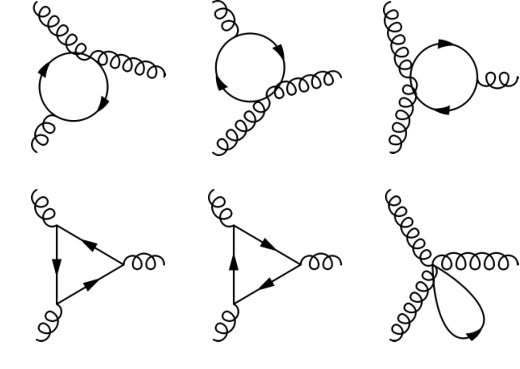
where $Z_{0}(\mathbf{k})=1+\mathcal{O}\left((ma)^{4}\right)$ is the residue of the pole of the tree-level gluon propagator at spatial momentum $\mathbf{k}$, and $m_{A}^{(0)}$ is defined so that the momentum $k$ is on-shell. We consider the dimensionless quantity $m_{A}^{(1)}/m$. The fermionic diagrams that contribute to this quantity are shown in figure 1 (a).

The anomalous dimension of $m_{A}$ is zero and so using Eqn. (11) we have $b^{(m_{A},1)}_{0,0}~=~0$. From gauge invariance we find $a^{(m_{A},1)}_{2,-2}~=~0$ and $a^{(m_{A},1)}_{0}(m_{q}a)=0$, which together with the previous result implies that $a^{(m_{A},1)}_{0,0}=0$.

The $\mathcal{O}\left(\alpha_{s}(ma)^{2}\right)$ contribution from improvement of the action is given by [7]

An effective coupling constant $\lambda$ for an AAB meson vertex is defined as

where we have factored out a twist factor of $\frac{i}{N}\mathrm{Tr}([\Gamma_{k},\Gamma_{p}]\Gamma_{q})$ from both sides, and the momenta and polarisations of the incoming particles are

Here $r>0$ is defined such that $E(\mathbf{q})=0$. This coupling is a spectral quantity since it can be related to the scattering amplitude of A mesons [10]. We expand Eqn. (14) perturbatively to one-loop order and find (up to $\mathcal{O}((ma)^{4})$ corrections)

The fermionic diagrams contributing to the irreducible three-point function $\Gamma^{(1)}$ are shown in figure 1 (b). Continuum calculations of the anomalous dimension and infrared divergence give

The improvement contribution to $\lambda$ is [7]

The external lines of the diagrams are on-shell, but with complex three-momentum $\mathbf{k}$; in the Euclidean formulation $k_{0}$ is also imaginary. In evaluating the loop integrals that are not pure tadpoles, care must be taken to ensure that the amplitudes calculated are the correct analytic continuations from the Minkowski space on-shell amplitudes defined with real three-momenta to the ones in Eqn. (15).

The situation is complicated by the presence of two mass scales $m,m_{q}$. The integrals are evaluated after performing a Wick rotation in $k_{0}$, taking care to avoid contour crossing of any poles that move as $r$ is continued from $r=0$ to $r=m/\sqrt{2}$. This requires $m_{q}/m>C$, where $C$ is a constant dependent on the graph being considered. After the Wick rotation in $k_{0}$, the (Euclidean) integration contour for $k_{0}$ (or, in one case, $k_{3}$) must be shifted by an imaginary constant.

To extract the improvement coefficients from our diagrammatic calculations, we compute the diagrams for a number of different values of both $L$ and $m_{q}$ with $N_{f}=1$, $N=3$. At each value of $m_{q}$, we then perform a fit in $ma$ of the form given in Eqn. (10) to extract the coefficients $a_{n}^{(Q,1)}(m_{q}a),~n=0,2$.

Performing a fit of the form (11) and (4), respectively, on these coefficients, we get the required coefficients of the $\mathcal{O}(a^{2})$ lattice artifacts in the chiral limit to be

These coefficients are to be identified with the $w_{i}$ of Eqn. (4).

Solving equation (4) for $c_{i}^{(1)}$, our results can be summarised as

where the quenched ($N_{f}=0$) results are taken from [7]. With $N_{f}=3$ the shift from the quenched values is surprisingly large, and may have a significant impact.

References

- [1] C. T. H. Davies et al., Phys. Rev. Lett. 92, 022001 (2004), [hep-lat/0304004].
- [2] C. Aubin et al., Phys. Rev. D70, 114501 (2004), [hep-lat/0407028].
- [3] K. Orginos, D. Toussaint and R. L. Sugar, Phys. Rev. D60, 054503 (1999), [hep-lat/9903032].
- [4] S. R. Sharpe, PoS LAT2006, 022 (2006), [hep-lat/0610094].
- [5] C. T. H. Davies, private communication.
- [6] M. Lüscher and P. Weisz, Nucl. Phys. B266, 309 (1986).
- [7] J. Snippe, Nucl. Phys. B498, 347 (1997), [hep-lat/9701002].
- [8] Zh. Hao, G. M. von Hippel, R. R. Horgan, Q. J. Mason and H. D. Trottier, arXiv:0705.4660 [hep-lat], to appear in Phys. Rev. D.
- [9] M. Lüscher and P. Weisz, Commun. Math. Phys. 97, 59 (1985).
- [10] M. Lüscher and P. Weisz, Phys. Lett. B158, 250 (1985).
- [11] A. Hart, G. M. von Hippel, R. R. Horgan and L. C. Storoni, J. Comput. Phys. 209, 340 (2005), [hep-lat/0411026].
- [12] H. D. Trottier, Nucl. Phys. Proc. Suppl. 129, 142 (2004), [hep-lat/0310044].
- [13] G. Parisi, Invited talk given at Summer Inst. Progress in Gauge Field Theory, Cargese, France, Sep 1-15, 1983.