Abundant stable gauge field hair for black holes in anti-de Sitter space

The “no-hair” conjecture wheeler states that black hole equilibrium states possess extremely simple geometries, determined completely by the mass, angular momentum and charge of the black hole. While hairy black hole solutions of the Einstein equations have been discovered, particularly in Einstein-Yang-Mills (EYM) theory and its variants (see volkov for a review), many of the plethora of new black hole solutions found in the literature are classically unstable. Those hairy black holes which are stable (such as the ${\mathfrak{su}}(2)$ EYM black holes in anti-de Sitter space (adS) ew; bjoraker) have, at least to date, been described by only a small number of parameters additional to the mass, angular momentum and charge of the black hole. This means that the “spirit” if not the “letter” of the no-hair conjecture is maintained.

In recent years there has been an explosion of interest in hairy black holes in adS, partly because at least some of these configurations are stable, but also because of the importance of the adS/CFT correspondence adsCFT in string theory. In particular, it has been suggested hertog that there should be observables in the dual (deformed) CFT which are sensitive to the presence of black hole hair (see also gauntlett for an adS/CFT interpretation of some stable seven-dimensional black holes with ${\mathfrak{so}}(5)$ gauge fields). Our purpose in this letter is to present new stable, asymptotically adS, hairy black hole solutions of ${\mathfrak{su}}(N)$ EYM for sufficiently large $\left|\Lambda\right|$ which are described by an unbounded number of parameters. The existence of these solutions casts the status of the “no-hair” conjecture in a completely new light: equilibrium black holes in adS are no longer simple objects, but rather require an infinite number of parameters in order to fully determine their geometry.

We consider static, spherically symmetric, four-dimensional black holes with metric

where the metric functions $\mu$ and $S$ depend on the radial co-ordinate $r$ only. Here, and throughout this letter, the metric has signature $(-,+,+,+)$ and we use units in which $4\pi G=c=1$. In the presence of a negative cosmological constant $\Lambda$, we write the metric function $\mu$ as

The most general, spherically symmetric, ansatz for the ${\mathfrak{su}}(N)$ gauge potential has been given in kunzle. Here, we assume that the gauge potential is purely magnetic and has the gauge-fixed form:

where $C$ is an $(N\times N)$ upper-triangular matrix with non-zero entries immediately above the diagonal:

for $j=1,\ldots,N-1$, with $C^{H}$ the Hermitian conjugate of $C$, and $D$ is a constant diagonal matrix:

The $(N-1)$ Yang-Mills equations take the form

for $j=1,\ldots,N-1$, where a prime ^′ denotes $d/dr$, and

with $\omega_{0}=\omega_{N}=0$. The Einstein equations take the form

where

The field equations (6,9) have the following trivial solutions. Setting $\omega_{j}(r)\equiv\pm{\sqrt{j(N-j)}}$ for all $j$ gives the Schwarzschild-adS black hole with $m(r)=M={\mbox{constant}}$ (which can be set to zero to give pure adS space). Setting $\omega_{j}(r)\equiv 0$ for all $j$ gives the Reissner-Nordström-adS black hole with magnetic charge. There is an additional special class of solutions, given by setting

In this case, it is possible to show, using a rescaling method along the lines of that in kunzle1, that the field variables $\omega(r)$, $m(r)$ and $S(r)$ satisfy the ${\mathfrak{su}}(2)$ EYM field equations with a negative cosmological constant. Furthermore, the boundary conditions (as discussed below) are also preserved. Therefore any ${\mathfrak{su}}(2)$, asymptotically adS, EYM black hole solution can be embedded into ${\mathfrak{su}}(N)$ EYM to give another asymptotically adS black hole.

In this letter we study black hole solutions of the field equations (6,9), returning to soliton solutions elsewhere suNsolutions. We assume there is a regular, non-extremal, black hole event horizon at $r=r_{h}$. The field variables $\omega_{j}(r)$, $m(r)$ and $S(r)$ will have regular Taylor series expansions about $r=r_{h}$. These expansions are determined by the $N+1$ quantities $\omega_{j}(r_{h})$, $r_{h}$, $S(r_{h})$ for fixed cosmological constant $\Lambda$. Since the field equations (6,9) are invariant under the transformation $\omega_{j}(r)\rightarrow-\omega_{j}(r)$ (for any $j$ independently), we may consider $\omega_{j}(r_{h})>0$ without loss of generality. For the event horizon to be non-extremal, it must be the case that

which constrains the possible values of the gauge field functions $\omega_{j}(r_{h})$ at the event horizon. At infinity, the boundary conditions are considerably less stringent than in the asymptotically flat case. In order for the metric (1) to be asymptotically adS, we simply require that the field variables $\omega_{j}(r)$, $m(r)$ and $S(r)$ converge to constant values as $r\rightarrow\infty$, and have regular Taylor series expansions in $r^{-1}$ near infinity. Since $\Lambda<0$, there is no cosmological horizon.

The field equations (6,9) are integrated numerically using standard ‘shooting’ techniques NR. The equation for $S(r)$ decouples from the other Einstein equation and the Yang-Mills equations so can be integrated separately if required. We start integrating just outside the event horizon, using as our shooting parameters the $N$ variables $\omega_{j}(r_{h})$ and $r_{h}$, subject to the weak constraint (12). The field equations are then integrated outwards in the radial co-ordinate $r$ until either the field variables start to diverge or they have converged to the asymptotic form at infinity.

As in the ${\mathfrak{su}}(2)$ case ew, we find black hole solutions in open subsets of the $N$-dimensional parameter space $\left(\omega_{j}(r_{h}),r_{h}\right)$ for fixed $\Lambda$. For sufficiently large $\left|\Lambda\right|$ (where how large “sufficiently large” is depends on the radius of the event horizon $r_{h}$), we find that the gauge field functions $\omega_{j}(r)$ all have no zeros. In figure 1 we show a typical nodeless solution, for ${\mathfrak{su}}(4)$ EYM.

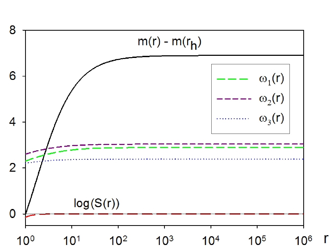
It can be seen that the metric functions $m(r)$ and $S(r)$ have very similar behaviour to the ${\mathfrak{su}}(2)$ case, and that, since $\left|\Lambda\right|$ is so large, the gauge field functions do not vary significantly from their values at the event horizon.

The phase space of black hole solutions in the ${\mathfrak{su}}(3)$ case, with $\Lambda=-10$ and $r_{h}=1$ is shown in figure 2, and is typical of the phase space for large values of $\left|\Lambda\right|$.

In figure 2 we have examined, for $\Lambda=-10$ and $r_{h}=1$, all values of the $\omega_{1}(r_{h})$ and $\omega_{2}(r_{h})$ which satisfy the constraint (12). The inequality in (12) is saturated on the outer-most curve in figure 2. It can be seen from figure 2 that not all values of $\left(\omega_{1}(r_{h}),\omega_{2}(r_{h})\right)$ give black hole solutions; those values for which no regular black hole solution satisfying the boundary conditions at infinity could be found lie in the narrow band on the outside of the plot. The region between this narrow band and the co-ordinate axes contains black hole solutions in which both gauge field functions $\omega_{1}(r)$ and $\omega_{2}(r)$ have no zeros. We have also plotted in figure 2 the line $\omega_{1}(r_{h})=\omega_{2}(r_{h})$, on which lie embedded ${\mathfrak{su}}(2)$ solutions given by (11). The significance of the shaded region in figure 2 will be described shortly. More detailed properties of the phase space of black hole solutions will be discussed elsewhere suNsolutions.

In ew, the existence of black hole solutions for which the gauge function $\omega(r)$ had no zeros was proven analytically in the ${\mathfrak{su}}(2)$ case. Since ${\mathfrak{su}}(2)$ solutions can be embedded as ${\mathfrak{su}}(N)$ solutions via (11), we have automatically an analytic proof of the existence of nodeless ${\mathfrak{su}}(N)$ EYM black holes in adS. However, these embedded solutions are ‘trivial’ in the sense that they are described by just three parameters: $r_{h}$, $\Lambda$ and $\omega(r_{h})$. An important question is whether the existence of ‘non-trivial’ (that is, genuinely ${\mathfrak{su}}(N)$) solutions in which all the gauge field functions $\omega_{j}(r)$ have no zeros can be proven analytically. The answer to this question is affirmative, and involves a generalization to ${\mathfrak{su}}(N)$ of the continuity-type argument used in ew. The details are lengthy and will be presented elsewhere. However, the main thrust of the argument can be simply stated. We firstly prove (generalizing the analysis of kunzle1 to include $\Lambda$) that the field equations (6,9) and initial conditions at the event horizon possess, locally in a neighborhood of the horizon, solutions which are analytic in $r$, $r_{h}$, $\Lambda$ and the parameters $\omega_{j}(r_{h})$. This enables us to prove that, in a sufficiently small neighborhood of any embedded ${\mathfrak{su}}(2)$ solution in which $\omega(r)$ has no nodes, there exists (at least in a neighborhood of the event horizon) an ${\mathfrak{su}}(N)$ solution in which all the $\omega_{j}(r)$ have no nodes. The key part of the proof lies in then showing that these ${\mathfrak{su}}(N)$ solutions can be extended out to $r\rightarrow\infty$ and that they satisfy the boundary conditions at infinity. This gives genuinely ${\mathfrak{su}}(N)$ black hole solutions in which all the gauge field functions have no zeros, and which are characterized by the $N+1$ parameters $r_{h}$, $\Lambda$ and $\omega_{j}(r_{h})$.

The other outstanding question is whether these new black holes, with potentially unbounded amounts of gauge field hair, are stable. We consider linear, spherically symmetric perturbations only for simplicity. Even for spherically symmetric perturbations, the analysis is highly involved in the ${\mathfrak{su}}(N)$ case and the details will be presented elsewhere. Here we briefly outline just the key features.

Firstly we consider spherically symmetric perturbations of the gauge potential (3), fixing the gauge so that the perturbed potential is purely magnetic and has the form kunzle

Here, the matrices ${\cal{B}}$ and $C$ depend on both $t$ and $r$, and matrix $D$ is still constant and given by (5). The matrix ${\cal{B}}(t,r)$ is traceless, diagonal and has purely imaginary entries. The only non-zero entries of the matrix $C(t,r)$ are:

As usual, the metric retains the form (1) but now the functions $m$ and $S$ depend on both $t$ and $r$. With this choice of gauge potential (13), the perturbation equations decouple into two sectors:

• •

  the sphaleronic sector consisting of entries of ${\cal{B}}$ and the functions $\gamma_{j}$;

• •

  the gravitational sector which consists of the perturbations of the metric functions $\delta m$ and $\delta S$ and the perturbations of the gauge field functions $\delta\omega_{j}$.

The form of the perturbation equations in the sphaleronic sector is little changed from the asymptotically flat case brodbeck. It consists of $2N-1$ coupled equations for the $2N-1$ variables ($N$ diagonal entries of the matrix ${\cal{B}}$ and $N-1$ functions $\gamma_{j}$). In addition, there is the Gauss constraint, which gives $N$ coupled consistency conditions. After much algebra (along the lines of brodbeck), the sphaleronic sector perturbation equations can be cast in the form

where a dot denotes $\partial/\partial t$, the $(2N-1)$-dimensional vector $\Psi$ consists of combinations of perturbations and ${\cal{U}}$ is a self-adjoint, second order, differential operator (involving derivatives with respect to $r$ but not $t$), depending on the equilibrium functions $\omega_{j}(r)$, $m(r)$ and $S(r)$. It can be shown that the operator ${\cal{U}}$ is regular and positive provided the unperturbed gauge functions $\omega_{j}(r)$ have no zeros and satisfy the $N-1$ inequalities

for all $j=1,\ldots N-1$. These inequalities define a non-empty subset of the parameter space, which is shown in the ${\mathfrak{su}}(3)$ case in figure 2.

The shaded region in figure 2 shows where the inequalities (16) are satisfied for the gauge field functions at the event horizon. However, the requirements of (16) are considerably stronger, as the inequalities have to be satisfied for all $r\geq r_{h}$. Our analytic work shows that, in fact, for sufficiently large $\left|\Lambda\right|$, there do exist solutions to the field equations for which the inequalities (16) are indeed satisfied for all $r$ (an example of such a solution is shown in figure 3).

This involves proving that for at least some solutions for which the gauge field function values at the event horizon lie within the region where the inequalities (16) are satisfied, the gauge field functions remain within this open region.

For the gravitational sector, the metric perturbations can be eliminated to yield a set of $N-1$, coupled perturbation equations of the form

where $\delta{\mbox{{\boldmath{{$\omega$}}}}}=\left(\delta\omega_{1},\ldots,\delta\omega_{N-1}\right)^{T}$, and ${\cal{M}}$ is a self-adjoint, second order, differential operator (involving derivatives with respect to $r$ but not $t$), depending on the equilibrium functions $\omega_{j}(r)$, $m(r)$ and $S(r)$. The operator ${\cal{M}}$ is more difficult to analyze than the operator ${\cal{U}}$. For sufficiently large $\left|\Lambda\right|$, it can be shown that ${\cal{M}}$ is a positive operator for embedded ${\mathfrak{su}}(2)$ solutions, provided that $\omega^{2}(r)>1$ for all $r$ (the existence of such ${\mathfrak{su}}(2)$ solutions is proved, for sufficiently large $\left|\Lambda\right|$, in ew). As described above, our analytic work ensures the existence of genuinely ${\mathfrak{su}}(N)$ solutions in a sufficiently small neighborhood of these embedded ${\mathfrak{su}}(2)$ solutions. These ${\mathfrak{su}}(N)$ solutions are such that the inequalities (16) are satisfied for all $r\geq r_{h}$ (and therefore the solutions are stable under sphaleronic perturbations). The positivity of ${\cal{M}}$ can then be extended to these genuinely ${\mathfrak{su}}(N)$ solutions using an analyticity argument, based on the nodal theorem of amann. The technical details of this argument will be presented elsewhere. Therefore at least some of our solutions are linearly stable in both the gravitational and sphaleronic perturbation sectors.

For sufficiently large $\left|\Lambda\right|$ (for each fixed $r_{h}$), we have shown the existence of ${\mathfrak{su}}(N)$ EYM black holes in adS, which are described by $N+1$ parameters and are stable under linear, spherically symmetric perturbations. If the cosmological constant is very large and negative, there are potentially a very large number of possible gauge field configurations giving the same mass and magnetic charge at infinity. As explained in the introduction, we anticipate that these solutions may well have interesting consequences for the adS/CFT correspondence adsCFT. We hope to return to these questions in the near future.