The quantum Chernoff bound as a measure of distinguishability between density matrices: application to qubit and Gaussian states
Abstract
Hypothesis testing is a fundamental issue in statistical inference and has been a crucial element in the development of information sciences. The Chernoff bound gives the minimal Bayesian error probability when discriminating two hypotheses given a large number of observations. Recently the combined work of Audenaert et al. [Phys. Rev. Lett. 98, 160501] and Nussbaum and Szkola [quant-ph/0607216] has proved the quantum analog of this bound, which applies when the hypotheses correspond to two quantum states. Based on the quantum Chernoff bound, we define a physically meaningful distinguishability measure and its corresponding metric in the space of states; the latter is shown to coincide with the Wigner-Yanase metric. Along the same lines, we define a second, more easily implementable, distinguishability measure based on the error probability of discrimination when the same local measurement is performed on every copy. We study some general properties of these measures, including the probability distribution of density matrices, defined via the volume element induced by the metric, and illustrate their use in the paradigmatic cases of qubits and Gaussian infinite-dimensional states.
pacs
03.67.Hk, 03.65.TaI Introduction
About fifty years ago Herman Chernoff proved his famous bound, which characterizes the asymptotic behavior of the minimal probability of error when discriminating two hypothesis given a large number of observations Chernoff 1952. Its quantum analog was recently conjectured Ogawa and Hayashi 2004 and finally proven by combining the results of two recent publications Audenaert et al. 2007a; Nussbaum and Szkola 2006. In this quantum setting one is confronted with the problem of knowing the minimum error probability in identifying one of two possible known states of which identical copies are given. Hereafter we will refer to this minimum simply as the error probability . This problem is widely known as quantum state discrimination 11 1 See J. A. Bergou and Hillery 2004 and Chefles 2000 for two reviews on the recent and more historical developments of this field respectively.. Its difficulty (but also its appeal) lies in the fact that quantum mechanics only allows for full discrimination of such states when they are orthogonal. This has both fundamental and practical implications that lie at the heart of quantum mechanics and its applications.
For these past fifty years the classical Chernoff bound —as well as hypothesis testing in general— has proved to be extremely useful in all branches of science. Likewise, one would expect its quantum version to be far more than a mere academic issue. The characterization and control of quantum devices is a necessary requirement for quantum computation and communication, and quantum hypothesis testing is specially designed for assessing the performance of these tasks. Particularly important examples for which state discrimination plays an essential role are quantum cryptography Gisin et al. 2002, classical capacity of quantum channels Hayashi and Nagaoka 2003, or even quantum algorithms Bacon et al. 2005. Equally important are some new theorems concerning different quantum extensions of hypothesis testing: the quantum Stein’s lemma, proved some years ago Hiai and Petz 1991; Ogawa and Nagaoka 2000, and the quantum Hoeffding bound, recently established in Nagaoka 2006; Hayashi 2006a; Audenaert et al. 2007b.
In this paper we study the classical and the quantum Chernoff bounds in connection to measures of distinguishability for quantum states, putting special emphasis on the qubit and Gaussian cases. We start by reviewing classical and quantum hypothesis testing and the corresponding Chernoff bounds in Sec. II and Sec. III, respectively (the latter includes the before mentioned recent results by Nussbaum and Szkola Nussbaum and Szkola 2006 and Audenaert et al. Audenaert et al. 2007a). In Sec IV we discuss the notion of a distinguishability measure for quantum states. We briefly motivate an important instance of such a notion based on classical statistical measures, that is, the quantum fidelity, and move to a fully operational alternative, based on the asymptotic rate exponent of the error probability in symmetric quantum hypothesis testing: the quantum Chernoff measure22 2 By ‘operational’ it is meant ‘defined though a specific procedure or task’, in contradistinction to ‘purely mathematical’. . We also discuss a similar distinguishability measure derived from the same rate exponent when the decision is based on identical single-copy (local) measurements —instead of the collective measurements on the copies assumed in the derivation of the quantum Chernoff bound. In Sec. V we study the metrics induced by the previously defined measures of distinguishability and give explicit expressions for general -dimensional systems. We also give the probability distribution of the eigenvalues of a density matrix based on the quantum Chernoff metric (induced by the corresponding distinguishability measure). We find that the metric based on local measurements is discontinuous and has to be defined piecewise: on the set of pure states, where it agrees with the Fubini-Study metric, and, separately, on the set of strictly mixed states, where it agrees with one-half the Bures-Uhlmann metric. The quantum Chernoff metric, in contrast, is continuous and smoothly interpolates between the Fubini-Study and one-half the Bures-Uhlmann metrics. In Sec. VI we concentrate on the particular case of two-level systems and study in some depth the differences between the quantum Chernoff measure and metric and those based on identical local measurements. In Sec. VII we give explicit expressions of the quantum Chernoff measure and its corresponding induced metric for general Gaussian states. Finally, we state our conclusions in Sec. VIII.
II Classical hypothesis testing: Chernoff bound
One of the most fundamental problems in statistical decision theory is that of choosing between two possible explanations or models, that we will refer to as hypothesis and , where the decision is based on a set of data collected from measurements or observations. For example, a medical team has to decide whether a patient is healthy (hypothesis ) or has certain disease (hypothesis ) in view of the results of some clinical test. Often, is called the working hypothesis or null hypothesis, while is called the alternative hypothesis. In general these two hypotheses do not have to be treated on equal footing, since wrongly accepting or rejecting one of them might have very different consequences. These two types of errors, i.e., the rejection of a true null hypothesis or the acceptance of a false null hypothesis, are called type I or type II errors respectively, and their corresponding probabilities will be denoted by and throughout the paper. In our example, failure to diagnose the disease is a type II error, whereas it is a type I error to wrongly conclude that the healthy patient has the disease. Of course it would be desirable to minimize the two types of errors at the same time. However, this is typically not possible since reducing those of one type entails increasing those of the other type. Hence, a common way to proceed is to minimize the errors of one type, while keeping those of the other type bounded by a constant (which may depend on the number of observations). Another (Bayesian-like) approach consists in minimizing a linear combination of the two error probabilities , where and can be interpreted as the a priori probabilities that we assign to the occurrence of each hypothesis. In this paper we consider this latter approach, which is known as symmetric hypothesis testing.
For the sake of simplicity, we assume to start with that , and we deal with tests that have only two possible outcomes, . This is, for example, the situation that corresponds to the identification of a biased coin that can be (with equal probability) of one of two types: or (corresponding to hypothesis or respectively). If it is of the type the probabilities of obtaining head and tail are respectively and , while if it is of type we write and . The test consists in tossing the coin, which has two possible outcomes: either head () or tail ().
If we can toss the coin only once (single observation), it is easy to convince oneself that the minimum (average) probability of error is attained when we accept the hypothesis (decide that the tossed coin is of the type) for which the observed outcome occurs with largest probability. Therefore 33 3 In this formula, as well as in most of the formulas involving minimization throughout the paper, one should properly write instead of since the minimum may not exist if and ( and in the quantum case) are degenerate and have different support. This is so because in this case the continuity of the argument of in all these equations is guaranteed only in the open interval and (end-point) singularities may occur at . We will overlook this mathematical subtlety in the main text to simplify the exposition.
| (1) | |||||
where we have used the inequality . The subscript CC stands for classical Chernoff. This expression also holds for tests with more than two outcomes. We just need to extend the sum over to the entire range of possible outcomes. In what follows, we leave the range of unspecified whenever an expression is valid for an arbitrary number of outcomes.
Next, let us assume we can toss the coin times. The set of possible outcomes (the sample space) is the -fold Cartesian product of (or ). The two probability distributions of these outcomes, and , will be given by the product of the corresponding single-observation distributions, , where now , and one immediately obtains Cover and Thomas 1991
| (2) |
This is the Chernoff bound Chernoff 1952. It is specially important because it can be proved to give the exact asymptotic rate exponent of the error probability, that is,
| (3) |
The so-called Chernoff information, or Chernoff distance, , can also be written in terms of the Kullback–Leibler divergence Cover and Thomas 1991:
| (4) |
where
| (5) |
is a family of probability distributions known as the Hellinger arc that interpolates between and , and is the value of at which the second equality in (4) holds. In other words, it is the point at which is equidistant to both and (in terms of Kullback–Leibler distance). It can be shown that is also the value of that minimizes the right hand side of (II).
For the case of measurements with two outcomes, such as the example of the coins discussed above, one can give a closed expression for the Chernoff distance, which we denote in this binary case as :
| (6) |
with
| (7) |
The parameter has a very straightforward interpretation. If is the number of heads (of ’s) after trials, which according to the distribution occurs with probability
| (8) |
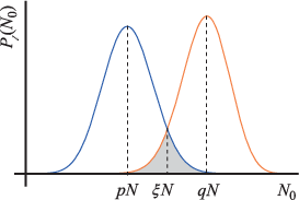
[according to the distribution it occurs with probability , defined the same way but with replaced by ], then is the fraction of heads above which one must decide in favor of . That is, if one accepts hypothesis , while if one accepts . Asymptotically, the contribution to the error probability is dominated by situations where , i.e., by events that occur with the same probability for both hypotheses (see Fig. 1). The probability of such events is clearly a lower-bound to the probability of error. It is straightforward to check that [or equivalently ] coincides with the upper bound given by the Chernoff distance . This proves that the Chernoff bound is indeed attainable.
III Quantum hypothesis testing: The quantum Chernoff bound
We now tackle discrimination (symmetric hypothesis testing) in a quantum scenario. We consider two sources, and that produce states described respectively by the density matrices and acting on a Hilbert space . We are given copies of a state with the promise that they have been produced either by the source (with prior probability ) or by the source (with prior probability ). Accordingly, we can formulate two hypothesis ( and ) about the identity ( or , respectively) of the source that has produced these copies. We wish to find a protocol to determine, with minimal error probability, which hypothesis better explains the nature of the copies. No matter how complicated this protocol might be, it is clear that the output must be classical: we have to settle for one of the two hypotheses. Therefore the protocol develops in two stages. First, to obtain information about the states we must necessarily make a (quantum) measurement, which in contrast to the classical world is an inherently random and destructive process. Second, one has to provide a classical algorithm that processes the measurement outcomes (classical data) and produces the best answer ( or ). Quantum mechanics allows for a convenient description of this two-step process by assigning to each answer, and , a single POVM (positive operator valued measure) element and respectively ( acts on ; ). The probability that this POVM measurement gives the answer conditioned to is .
The problem thus reduces to finding the set of operators that minimize the mean probability of error, For the simplest case of a single copy () and two equiprobable hypotheses () it is Helstrom 1976
| (9) |
Since , we can introduce the Helstrom matrix , as is common in quantum state discrimination, and write
| (10) |
which only needs to be optimized with respect to . We note that has some negative eigenvalues, as . This necessarily implies that the minimum error probability is attained if is the projector on the subspace of positive eigenvalues of . We will denote this projector by and define the positive part of as . Taking into account that is traceless, we obtain
| (11) |
where the matrix (absolute value of ) is defined to be . We arrive at the final result Helstrom 1976,
| (12) |
The problem of discriminating multiple copies (arbitrary ) is thus formally solved by replacing by in the above equations. Indeed, if we do not have any restrictions on the type of measurements performed on the copies, , and the mean probability of error is just
| (13) |
However, the computation of the trace norm of the Helmstrom matrix in (13) is tedious and, moreover, this equation provides little information about the large behavior of the error probability, which is what the Chernoff bound is about.
The quantum version of the Chernoff (upper) bound was presented very recently in Audenaert et al. 2007a. There it is shown that
| (14) |
(the subscript QC stands for quantum Chernoff), which holds for arbitrary density matrices. Moreover, this bound can be very efficiently computed.
The bound (14) is a straightforward application of the following theorem Audenaert et al. 2007a:
Theorem 1
Let and be two positive operators, then for all ,
| (15) |
The proof of this theorem involves advanced methods in matrix algebra and we refer the interested reader to Audenaert et al. 2007a. Instead, here we will give a simple proof of the inequality (14) where instead of minimizing over , the particular value will be chosen.
We first notice that one obtains an upper-bound to by picking any particular positive operator (and, accordingly, ) in (9). A convenient choice is (and thus ), where, as above, stands for the projector onto the subspace spanned by the eigenstates of with positive eigenvalue. After the following series of inequalities we arrive to the desired result Hayashi 2006b:
| (16) | |||||
where in the second inequality we have used
| (17) |
The general proof (for all ) follows the same steps but taking if and if . In this case, the inequality analogous to the second one in (16) requires the two additional non-obvious relations
| (18) |
These inequalities follow immediately from the following non-trivial lemma, which constitutes the core of the proof Audenaert et al. 2007a:
Lemma 1
Let and be two positive operators, then for all ,
| (19) |
Before proceeding with the the asymptotic limit, several comments about (14) are in order. (i) The exponential fall-off of the probability of error when a number of copies is available follows immediately from :
| (20) |
Remarkably enough, this rate exponent, which we may call quantum Chernoff information because of its analogy with , is asymptotically attainable, as follows from the results of Nussbaum and Szkola 2006. This is the quantum extension of the classical result (II) and was first conjectured by Ogawa and Hayashi in Ogawa and Hayashi 2004. (ii) If the two matrices and commute the bound reduces to the classical Chernoff bound (1), where the two probability distributions are given by the spectrum of the two density matrices. (iii) The function (whose minimum gives the best bound) is a convex function of in , which means that a stationary point will automatically be the global minimum (see Audenaert et al. 2007a for a proof). This is a very useful fact when computing the quantum Chernoff bound (14). (iv) is jointly concave in , unitarily invariant, and non-decreasing under trace preserving quantum operations Audenaert et al. 2007a. (v) The quantum Chernoff bound gives a tighter bound than that given by the quantum fidelity
| (21) |
which is the most widely used quantum distinguishability measure (see next section). This follows from the following set of inequalities:
| (22) |
In fact, the fidelity also provides a lower-bound to the probability of error Fuchs and de Graaf 1999:
| (23) |
In the case where one of the states (say ) is pure the upper bound to the error probability can be made tighter Nielsen and Chuang 2000; Kargin 2005:
| (24) |
(vi) The quantum Chernoff bound can be easily extended to the case where the two states and (sources) are not equiprobable:
| (25) |
(vii) The permutation invariance of the -copy density matrices, , guarantees that the optimal collective measurement can be implemented efficiently (with a polynomial-size circuit known as quantum Schur transform) Bacon et al. 2006, and hence that the minimum probability of error is achievable with reasonable resources.
As stated above, for multiple-copy discrimination the error probability decreases exponentially with the number of copies: as goes to infinity Cover and Thomas 1991. The error (rate) exponent is defined generically by
| (26) |
and characterizes the asymptotic behavior of the error probability. From (20) we readily see that if the best (joint) measurement is used it coincides with the quantum Chernoff information,
| (27) |
where the equality holds because of the attainability of (20) discussed above and we have added the subscript QC. Moreover, this asymptotic value is also attained by the square root (or “pretty-good”) measurement (see Holevo 1979; Hausladen et al. 1996 for the precise definition). This immediately follows from the known bounds Barnum and Knill 2002; Harrow and Winter 2006 , where is the error probability of discrimination when the square root measurement is used.
Before closing this section, we briefly come back to the fidelity bounds in (22–24) and simply note that the first two inequalities translate into the following bounds to the rate exponent:
| (28) |
If one of the states is pure Eq. (24) implies that the factor in (28) becomes and we have the exact relation
| (29) |
IV Distinguishability measures
In this section we aim to define a measure of distinguishability between states using the results reviewed in Sec. III. Before doing so we will briefly outline how classical statistical methods can be used to (partially) accomplish this goal. We will then discuss an operational measure of distinguishability based on the error probability in multiple-copy state discrimination, leading to the quantum Chernoff measure. Finally we will define the analogous quantity for local discrimination protocols.
IV.1 Classical statistical approach
The notion of distance between states is a fundamental issue that has been studied for a long time. A straightforward way to define such a distance is to take any suitable norm in the space of states. However, a more physical approach, kick-started by the pioneering work in Wootters 1981, is to relate the inherently probabilistic nature of quantum measurements to classical statistical measures of distinguishability between probability distributions.
In particular, the author in Wootters 1981 uses the notion of statistical distance,
| (30) |
as a measure of distinguishability between the probability distributions and , where
| (31) |
is the statistical fidelity. Accordingly, he defines a distinguishability measure between quantum states and by maximizing [i.e., minimizing ] over all possible POVM measurements, characterized by all possible sets of operators with outcome probabilities given by and . The statistical distance as such makes sense only when the number of samplings of the probability distribution is large. Hence, in the quantum extension of this notion it is implicitly assumed that one performs the same measurement on each of a large number of copies of the state . The optimization over such local repeated measurements leads to one of the most widely used distinguishability measures Fuchs 1996: The (quantum) fidelity , defined in (21).
The fidelity, or statistical distance, has many desirable properties: (i) it is easily computable; (ii) for pure states it reduces to the standard distance given by the angle between rays in the Hilbert space ; (iii) as mentioned above, it provides bounds to . Nevertheless, a strict physical interpretation is so far unclear, and its definition is based on repeated local measurements, while quantum mechanics allows for much more general ways to access the information contained in the copies, via collective measurements on the whole of them.
IV.2 Quantum Chernoff distance
A very natural and also operational distinguishability measure is provided by the error probability of discrimination. As a first candidate, one could take this very error probability for a given fixed number of copies. However, the choice of a particular in such a definition would not only be arbitrary but also problematic since one can find examples Cover and Thomas 1991 where , whereas for a different number of copies. A straightforward way to go around this problem is to use the asymptotic expressions for and define the distinguishability measure as the largest rate exponent in (26). We further note that the presence of the logarithm ensures that if and only if , while the minus sign makes distinguishability decrease as discrimination becomes more difficult, i.e., as increases.
The quantum Chernoff information, , is therefore a physically meaningful and efficiently computable distinguishability measure. Note that (27) does not stricto sensu define a distance, since it does not fulfil the triangular inequality. It has however all of the other properties that one should expect from a reasonable measure. This, in itself, is already a remarkable fact since, as far as measures and metrics are concerned, there is usually a compromise among operational definiteness, computability and contractivity Gilchrist et al. 2005. For instance, the distance proposed in Lee et al. 2003, although having an operational definition, is not contractive.
We point out that another operational distinguishability measure can be obtained in asymmetric hypothesis testing by minimizing the type II error rate while keeping the type I error rate upper-bounded by a fixed value. The optimal error rate in this situation is provided by the quantum Stein’s Lemma Hiai and Petz 1991; Ogawa and Nagaoka 2000 and leads to the well known quantum relative entropy. Despite of having an operational meaning, the quantum relative entropy has two obvious drawbacks as a distinguishability measure: it is not symmetric on its arguments and it diverges if one of the states is pure.
IV.3 Classical Chernoff distance: local measurements
In the derivation of the quantum Chernoff bound one optimizes over all possible quantum measurements, in particular over quantum joint measurements on , that act over all the copies coherently. It is of great interest, both theoretically and in practice, to know whether such joint measurements are strictly necessary to attain the bound or one can make do with separable ones (which include those that can be implemented with local operations and classical communication, simply known as LOCC measurements). As far as we are aware, the answer to this is unknown. This question is also relevant in connection with the operational meaning attached to . In this section we focus on this operational aspect and compute from its definition in (26) assuming that the discrimination protocol refers to is constrained to make use of the same individual measurements, defined by a local POVM , on each of the available copies. We loosely refer to these protocols as local. Local protocols are relevant from the theoretical point of view since they help to elucidate the role of quantum correlated measurements in asymptotic hypothesis testing. For example, in quantum phase estimation local measurements suffice to achieve the collective bounds Holevo 1979. Here, we will show that these protocols do not achieve the quantum Chernoff bound. In addition, from a more practical point of view, local protocols are much simpler to implement experimentally, specially in a situation where the number of sub-systems is increasingly large.
In such a local protocol, after the measurements have been performed we have a sample of elements of the probability distribution , , based on which we have to discriminate between the candidate or . In such a scenario the error probability, which we call , can be obtained using the classical Chernoff bound (1) applied to the distributions and . One can thus define the error exponent (26) and thereby introduce a new operational distinguishability measure based on local discrimination:
| (32) |
where the subscript reminds us that we have made use of the classical Chernoff bound.
The measure is obtained by maximizing the rate exponent over all possible single-copy generalized measurements (just as is done for the fidelity). Unfortunately, there is no simple closed expression for this maximum for general mixed states. However, we do encounter again the relation (22) with the fidelity: since the square root of the statistical fidelity upper bounds in (1), it also upper bounds the local error probability . That is,
| (33) |
and
| (34) |
Since , we note that whenever the inequality (34) has to be saturated. This, in turn, means that in this situation one can optimally discriminate between and just by performing a fixed local measurement on each of the copies (no collective measurements are required to attain the quantum Chernoff bound).
There is still another important situation when the quantum Chernoff bound is attainable by local measurements: when one of the states (say ) is pure. If this is the case, Eq. (24) holds and . To prove that , let us consider the two-outcome measurement defined by , . Note that and . After performing this measurement on each of the copies the protocol proceeds as follows: we accept if all of the outcomes are , otherwise we accept . One may refer to this classical data processing as unanimity vote Acin et al. 2005. The error probability can be easily computed by noticing that no error occurs unless we get times the outcome [since ]. Therefore,
| (35) |
where the last equality holds because is assumed to be a pure state. From this equation it follows immediately that , and the quantum Chernoff bound is attainable by local measurements. It also follows from the first equality in (35) that this result corresponds to taking the limit in (1).
V Metric
The set of states of a quantum system, as that of classical probability distributions on a given sample space,44 4 For sake of clarity, in this section we assume a finite sample space, but the results hold also for general probability measures over continuous spaces. can be endowed with a metric structure Bengtsson and Życzkowski 2006, and thus thought of as a Riemannian manifold. This enables us to relate geometrical concepts (e.g., distance, volume, curvature, parallel transport) to physical ones (e.g., state discrimination and estimation, geometrical phases). Among the novel applications of metrics in quantum information, they have been recently used to characterize quantum phase transitions Zanardi et al. 2007.
The first step towards this geometric approach to quantum states is to define the line element or (infinitesimal) distance between two neighboring “points” and . All local properties follow from this definition. More precisely, they follow from the metric, i.e., from the set of coefficients of when written as a quadratic form in the differentials of the coordinates (parameters) that specify the quantum states. There is, however, no unique choice of unless some monotonicity conditions are invoked.
For classical probability distributions, , a line element is singularized (up to a propotionality factor) by imposing that it be non-increasing under stochastic maps. It is the well known Fisher metric (in what follows the terms metric and line element will be used interchangeably):
| (36) |
In contrast to the classical case, the monotonicity condition under completely positive (quantum stochastic) maps does not define a metric uniquely, which explains why a substantial body of research on quantum metrics has emerged over the last years. Among the main developments, Petz Petz 1996 has characterized the family of quantum contractive metrics by establishing a correspondence with operator-monotone functions.
An alternative, more physical approach is to define a line element from a suitable distinguishability measure between infinitesimally close states. A remarkable example is given in Braunstein and Caves 1994. In this seminal paper Braunstein and Caves consider a one-parameter family of states and map the problem of distinguishability to that of estimating the parameter optimally. They define a line element, , as expressed in the appropriate units of statistical deviation (roughly speaking, divided by the minimal error in the estimation of ). By making use of classical statistical methods (Cramér-Rao bound) they find
| (37) |
where (it is the so called Fisher information), with , and the maximization is over all possible POVM measurements on a single copy of . They also succeed in giving a closed expression for and show that their metric coincides up to a factor with that induced by the Bures-Uhlmann distance Bures 1969; Uhlmann 1976
| (38) |
More precisely, they show that , where
| (39) |
[see also (69) below] and a series expansion to is understood in the right hand side of this equation. We note in passing that for commuting states, i.e., classical probability distributions, the Bures-Uhlmann line element coincides with the Fisher metric (36). A quantum metric with such normalization is said to be Fisher adjusted.
Although one can obtain a finite distance for arbitrary states and by integrating along geodesics, it is important to notice that the operational meaning of the Braunstein and Caves metric is lost in the process.
In the spirit of Braustein and Caves’ physical approach to metrics, we next consider the distinguishability measures and , discussed in Section IV, for infinitesimally close states and derive line elements with the same operational meaning, which we call and respectively. For we also give the volume element and the prior probability distribution, whereas those corresponding to the metric can be easily found in the literature since, as will be shown, is proportional to the widely-studied Bures metric .
Before we start we would like to point out that one could also consider line elements induced by other quantities, such as the quantum relative entropy, which, as we saw above, also has a clear operational interpretation. The quantum relative entropy induces the so-called Kubo-Mori metric Petz 2002, which has the drawback of being singular for pure states.
V.1 Quantum Chernoff metric
For neighboring density matrices and (e.g., those for which their independent matrix elements differ by an infinitesimal amount) the distinguishability measure defines a metric, as in (39). For the quantum Chernoff measure, , this metric can be computed from Eq. (27) Audenaert et al. 2006:
| (40) |
where the dots stand for higher order terms in that will not contribute to and we have also used that . We now recall the integral representation
| (41) |
and its derivative,
| (42) |
These representations hold for and can be straightforwardly extended to positive matrices. In particular, using (41) and the convergent sequence
| (43) |
which also holds for matrices provided , one can write, up to second order in ,
| (44) | |||||
where . Inserting this expansion in (40) one finds
| (45) | |||||
The first term in the integrand vanishes, as can be seen by using (42) and , while the second term can be computed in the eigenbasis of ; :
| (46) | |||||
where in the second equality we have taken into account that , which enabled us to symmetrize the expression in parenthesis that multiplies in the sum (this symmetrization gives the factor ). The quantum Chernoff metric can be finally written as,
| (47) |
The quantum Chernoff metric belongs to the family of contractive quantum metrics, as it should, since by construction the probability of error cannot be improved by a pre-processing of the states. In fact the quantum Chernoff metric coincides with a member of this family that has been explicitly written by Petz in Petz and Sudár 1999 and with the so called Wigner-Yanase metric, which has been recently studied in depth by the authors of Gibilisco and Isola 2003. In particular, the geodesic distance, the geodesic path, and the scalar curvature of the quantum Chernoff metric can be read off from their Eqs. (5.1-5.3).
By separating diagonal from off-diagonal terms, the metric in (47) can also be written as
| (48) |
Next, we wish to identify the degrees of freedom in the off-diagonal terms. We will see that they correspond to infinitesimal unitary transformations acting on (which leave its eigenvalues unchanged). This is most conveniently done by parameterizing by its eigenvalues and eigenvectors, namely by and the components of onto a given canonical basis :
| (49) |
(naturally, it also holds that ). A neighboring density matrix is thus parameterized by and . We further note that , where is antihermitian, . It is actually the infinitesimal generator along the direction in parameter space that takes into . It follows that . The matrix elements of can be expressed as
| (50) | |||||
and those of as
| (51) | |||||
where we have used (49) in going from the first to the second line [the very same matrix elements of can also be written as in the eigenbasis of ]. Substituting these relations back into (48) we obtain
| (52) |
The same expression can also be derived by differentiating
| (53) |
where is diagonal in the canonical basis and has the spectrum of .
Eq. (52) displays the metric in a very suggestive form. Any density matrix can be parameterized by its eigenvalues and the unitary matrix that diagonalizes it. Eq. (52) expresses the infinitesimal distance between two such matrices in terms of these very parameters. The first term is immediately recognized as the (Fisher) metric on the -dimensional simplex of eigenvalues of , which is assumed to be throughout the rest of this section (note that , which implies ). Thus, stricto senso, it should be expressed in terms of a set of independent eigenvalues. If we choose this set to be the first term in (52) becomes
| (54) |
where the subscript stands for Fisher, and
| (55) |
It follows that the determinant of , which we will need below, is
| (56) |
The second term in (52) contains the factors , which are invariant under left-multiplication [since the left-hand side of (51) is independent of the choice of basis ]. Hence, the normalized volume element induced by these terms will coincide with the (unique) Haar measure of , known as the flag manifold (see e.g., Życzkowski and Sommers 2001 and references therein). Using the wedge product of differential forms, this Haar measure can be written as
| (57) |
where is a normalization constant so that . Note that the one-form basis in (57) contains (real and independent) elements, which indeed coincides with the independent parameters of .
Volume elements (derived from metrics) are of great interest because they give a canonical way of defining prior probability distributions on continuous sets. According to this approach, Eqs. (52–57) provide a means to define such probability distribution for general density matrices: if is a set of independent real parameters that specifies the density matrices as and the metric is written as (i.e., is the metric tensor), then we can define the prior through the relation , where . It follows from (52) that is the product of two independent probability distributions: one that depends exclusively on the parameters encoded in the unitary matrix and expresses the fact that they are simply distributed according to the Haar measure ; and one, denoted as , that gives the probability distribution of eigenvalues. The latter can be written as
| (58) |
where for a given dimension the constant is chosen to ensure that probability adds up to one.
The prior distribution on the simplex of eigenvalues of for the Bures metric (see below), analogous to in (58), was proposed in Hall 1998, but it took considerable efforts to compute the right normalization constant. Slater Slater 1999 gave values for dimensions and finally Sommers and Życzkowski Sommers and Życzkowski 2003 managed to give a general expression for arbitrary finite dimensions. Here we will compute following similar techniques.
The coefficient is defined by the normalization condition . Thus, , where
| (59) |
Although we only need this integral for , the introduction of this radial parameter enables us to compute the normalization more easily. We first note that by re-scaling one gets
| (60) |
[i.e., is a homogeneous function of of degree ], and thus
| (61) |
It follows from this equation that
| (62) | |||||
This expression can be further simplified by the change of variables , which leads to
| (63) |
By expanding the square of the Vandermonde determinant , one could in principle compute in terms of Euler gamma functions. However this is very impractical since the number of terms in such an expansion grows exponentially with . A much more efficient way to proceed is as follows. Let , , be a family or orthonormal polynomials in the set with a weight function of Hermite type, so that
| (64) |
Note that are not Hermite polynomials, since the integration range is instead of . Now, if we define the renormalized polynomials it is not hard to show that
| (65) |
Substituting in to (63) and using the orthonormality of , one has
| (66) |
In contrast to the examples considered in Ref. Sommers and Życzkowski 2003, and as far as we are aware, there is no known closed expression for the leading coefficients for the case at hand. However, Eq. (66) provides an efficient way of computing the quantum Chernoff normalization constant ; e.g., by applying the Gram-Schmidt orthogonalization algorithm [with the internal product defined in Eq. (64)] one easily obtains the coefficients , and thereby . We give the value of this constant for :
| (67) |
V.2 Classical Chernoff/Bures metric
From the local measure , Eq. (32), one can readily obtain the corresponding local metric. If for every measurement outcome , direct differentiation of leads to
| (68) |
where is the Fisher metric (36), with , and being the value of that achieves this minimum in (32). The maximization of (36) over the local measurements , which commutes with the minimization over as long as , results in Braunstein and Caves 1994
| (69) |
or equivalently,
| (70) |
where we use the same notation as in (47) and (52), respectively. This is the Bures-Uhlmann metric, which, as mentioned above, can be also obtained from the Bures distance (38) Hübner 1992. From (68) we then have
| (71) |
for strictly mixed states (the last equality holds to order ). The corresponding prior probability distribution (quantum Jeffreys prior) was derived and calculated in Hall 1998; Slater 1999; Sommers and Życzkowski 2003.
If one of the states is pure (say , as in previous sections) then the classical distribution becomes degenerate [] for the optimal choice (recall the last comments in Sec. IV.3), and the previous derivation does not hold. In this case, the optimal choice of in (1) is obtained by taking the limit , as we already discussed in Sec. IV.3. Recalling the first equality in (35), we obtain [note that since ], which is linear in and therefore does not define a proper metric in probability space. From the results of Sec. IV.3 we also know that if one of the states is pure then and therefore
| (72) |
for pure states. This agrees with the previous discussion since if is a pure state. Eq. (72) has to be taken with special care. It gives a valid metric for the set of pure states (which only includes variations in the unitary parameters), i.e., when is also a pure state (). Moreover, for pure states coincides with the Fubini-Study metric [recall that the Bures-Uhlmann metric is Fubini-Study adjusted Sommers and Życzkowski 2003, hence this statement follows from Eq. (72)].
By combining Eqs. (71) and (72), we see that shows a discontinuity when the mixed state approaches the set of pure states. The quantum Chernoff metric (47) does not have this pathology. This can be seen by comparing the () terms in (52) with those in (70) (the diagonal terms coincide). As ( approaches a pure state), we readily see that . In the opposite situation, when approaches the completely mixed state , we can write , where approaches zero. Expanding the terms in both (52) and (70) we can check that up to terms of order . We conclude that the quantum Chernoff metric smoothly interpolates between the two components (that on strictly mixed states and that on pure states) of the local metric . We will come back to this point in the next section, where qubit states are discussed as an example to illustrate the results in this and in previous sections.
VI Qubit states
In this section we apply our results to qubit mixed states, that is, general two-dimensional states. We will first study the distinguishability measures and and then move on to the corresponding metrics and priors.
For qubits one has , , where is the Bloch vector of , . The eigenvalues of are and . It is straightforward to obtain
| (73) | |||||
where is the angle between and . The value of that minimizes and hence gives (14) and (27) is in general a function of and . However, one can check that in the particular case the minimum is at 55 5 Qubit states are an example for which the doubly stochastic matrix is symmetric (). Therefore, for isospectral states, , which has its minimum at ..
In Fig. 2 we plot the quantum Chernoff distinguishability measure and the measure based on local measurements together with the bounds (28) provided by the fidelity, for states of equal purity and for .
Notice that in general local measurements perform much worse than the collective ones and runs remarkably close to (actually, coincides with) the fidelity lowerbound (28) for most values of . However, as it approaches the pure-state regime () it rapidly increases towards its upper-bound. The reason for this rapid change can be understood by recalling the unanimity vote protocol discussed in Sec. IV.3. For two pure states, (as corresponds to ), it boils down to Acin et al. 2005 projecting along one of the states, say , and its orthogonal, . After performing this measurement on each of the copies, if all of them project on , one claims that the unknown state is (hypothesis ). However, if at least one of them projects on the guess is (one accepts ). This corresponds to in (7). For pure states it reaches the joint-measurement Chernoff bound by making use of a much less demanding local-measurement protocol (see also Brody and Meister 1996; Acin et al. 2005 for the optimal local strategy for finite ).
In contrast, near the completely mixed state , for low , the optimal local strategy consists in choosing the measurement such that , with . In this case, the acceptance of either or is done on the basis of a majority vote protocol: is accepted if the outcome occurs more times than the outcome does, i.e, [see also Eq. (7)]. It follows from (4) that . Therefore, the lower-bound provided by the fidelity, Eq. (28), is saturated [ saturates the second inequality in (33) and thus it also saturates (34)]. This protocol is optimal up to a given value of the purity, i.e., for . For larger values of the ‘voting rule’ (given by ) starts changing and so does . Accordingly, moves away from its lower-bound to end up saturating its upper bound at .
We next consider the metrics induced by local and by joint measures. The former, in particular, requires special attention because of the abrupt behavior of near the set of pure states. Indeed the critical value , beyond which majority vote is no longer optimal, goes to one as the relative angle between the Bloch vectors of the states becomes smaller; as . As a result, the sudden increase of develops into a jump discontinuity at [from if to if ]. For this reason, when defining the corresponding metric we have to distinguish these two regions: the set of strictly mixed states () and the set of pure states ().
In the region the outcome probabilities will never be degenerate and the metric reduces to the Fisher metric, which upon optimization over local measurements coincides with one-half the Bures metric:
| (74) |
where is the usual metric on the 2-sphere.
In the region (pure states), the before-mentioned unanimity vote protocol is optimal and the resulting metric is
| (75) |
where is the well known Fubini-Study metric, which, as mentioned above, also coincides with the Bures metric in the limiting case . We notice again that in Eq. (75) is a factor larger than in Eq. (74), where the limit is taken along the lines . The local distinguishability measure thus induces a discontinuous metric or, phrased in a different way, two different metrics for pure states or for strictly mixed states.
This can be visualized using the Uhlmann representation, that is, by embedding the Bloch sphere in . To this end, one simply needs to define the new coordinate as , where . In spherical coordinates one has
| (76) |
where the first line correspond to strictly mixed states and the second to pure states. We note that in the second (first) line is nothing but the standard metric on a 2-sphere (the top half of a 3-sphere) of radius ().
In Fig. 3, and represent (the slice of) these two manifolds. One readily sees that the radius of (pure states) is a factor larger than that of the limiting circle of (for , i.e., ).
The quantum Chernoff (collective-measurement based) metric can be readily obtained from (27) [or (52) particularized to qubit mixed states]:
| (77) |
This metric quantifies distinguishability of qubit states in a precise and operational way, and encapsulates the full power of quantum mechanics. It approaches the Fubini-Study metric for pure states and also for very mixed states, i.e. for small . The metric smoothly interpolates between the two regimes. By defining with we obtain again the standard metric on a 3-sphere but this time of radius :
| (78) |
The corresponding manifold is denoted by in Fig. 3. Geometrically the space of states endowed with the quantum Chernoff metric is a spherical cap defined by whose radius is twice that of the Bures-like hemisphere . In order to emphasize that the two metrics, are equal up to order at , i.e., (near ), in the figure we have shifted the center of the larger sphere so as to make the two manifolds tangent at . The fact that is a particular example of a general relation that we discussed at the end of Sec. V.2.
From the quantum Chernoff metric one can obtain a proper finite distance (satisfying the triangle inequality) by, for example, computing the geodesic distance,
| (79) |
where and is the relative angle between the respective Bloch vectors.
The volume element and the prior distribution of density matrices for qubit mixed states, which we here denote as , can be easily obtained from the above metrics. According to the local and quantum Chernoff metrics we have respectively:
| (80) | |||||
| (81) |
where it is understood that and are the length and the azimuthal angle of the Bloch vector of . Since the Haar volume density on the 2-sphere is , we see that the eigenvalues of , are distributed according to
| (82) | |||||
| (83) |
(One can check that the latter agrees with our results in Sec. V.) This have been recently used in de Burgh et al. 2007 to assess the accuracy of different quantum tomographic measurements.
VII Gaussian States
We now illustrate our results with infinite-dimensional systems. In particular we will focus on the family of single-mode Gaussian states. This is a very significant class of quantum states mainly for two reasons. First, it has a very simple mathematical characterization that allows for the derivation of otherwise highly non-trivial results, and, second, it describes accurately states of light that are realized with current technology. In the following we show that the Quantum Chernoff information, besides being the natural distinguishability measure, has the advantage of being relatively easy to compute. The calculation of the fidelity, for instance, is much more involved, as is apparent from Abe 1999; Twamley 1996; Paraoanu and Scutaru 1998; Wang et al. 1998; Slater 1996, where one can find such calculations for different classes of gaussian states.
Gaussian states are by definition those that have a gaussian characteristic function. The (symmetrically ordered) characteristic function of one such state, , is:
| (84) |
where denotes transposition, is the symplectic matrix
| (85) |
and is the displacement operator, with and with position and momentum operators satisfying . The annihilation and creation operators, defined as and , fulfil the canonical commutation relations. The positivity of implies that the covariance matrix is real-symmetric and satisfies . A symplectic transformation is a linear transformation that preserves the commutation relations, or more succinctly . Under such a transformation the displacement vector and the covariance matrix transform as as respectively.
An equivalent, more physical, definition can be given by the action of the squeezing operator and the displacement operator defined above, on a thermal state , where the Fock states satisfy :
| (86) |
The covariance matrix of a thermal state is simply , with . The squeezing operator induces the symplectic transformation , where
| (87) |
and the latter corresponds to a rotation in phase-space, i.e. to the unitary operation . One thus finds that the covariance matrix can be written as .
In order to calculate the Chernoff bound it is sufficient to realize that any power of any Gaussian state is also a Gaussian (unnormalized) state with a rescaled temperature:
| (88) | |||||
where we have used the relation
| (89) |
with . Recall now that given any two gaussian states and , one can write the inner product in terms of their displacement vectors and covariance matrices as:
| (90) |
where . Using this equation we find that the quantum Chernoff bound (14) is with
| (91) | |||||
where , , and . To simplify the notation we will denote the covariance matrix of the Gaussian state with as .
VII.1 States with equal covariance matrices
If two general Gaussian states and are identical modulo a relative displacement , i.e. we find that
| (92) |
where in the first equality we used the fact that the factor multiplying the exponential in (92) must be equal to one, since it is independent of and for one must have , which implies that . That is,
| (93) | |||||
where we have used that symplectic transformations have unit determinant, i.e., . One readily sees that , Eq. (92), attains its minimum at , hence we find that in this case the Chernoff measure is:
| (94) | |||||
where is the relative angle between the squeezing axis and the displacement vector, i.e., if then .
VII.2 States with the same temperature
We can generalize the previous result to states that have the same spectra, i.e., the same temperature (). In this case we can use (93) to find
| (95) | |||||
The determinant can be explicitly written in a compact form as
| (96) | |||||
where we have defined
| (97) |
with
| (98) | |||||
With this generality , the optimal value of , is a complicated function of the states’ parameters 66 6 In contrast to the claims in Exercise 3.9 page 77 of Hayashi 2006b, it is not generally the case that for states with equal spectra the minimum of is reached for .. In the case of , i.e., states with no relative displacement and the same temperature, the minimization over can be done analytically, and one finds . The quantum Chernoff measure becomes:
| (99) | |||
Notice that this expression is independent of the temperature (or purity) of the states. That is, the distinguishability of two arbitrary Gaussian states with no relative displacement and equal temperature is independent of the degree of mixedness of the states.
VII.3 Chernoff metric for Gaussian states
Following the definition (40) and using the previous results we find that Chernoff metric is
| (100) | |||||
where we have defined the rotated displacement variables and we have used that for infinitesimal changes . We find again that the metric is independent of the temperature under variations of the squeezing parameters and .
The (unnormalized) quantum Jeffreys prior can be obtained from the metric tensor:
| (101) |
The metric induced by the local measure on the set of mixed states is given by one-half the Bures metric 77 7 There seems to be a typo in Kwek et al. 1999 in the contribution of small displacements of Eq. (13).
| (102) | |||||
We note that, as approaches the set of pure states () along the lines , in agreement with the general statement at the end of Sec. V.2. In the limit of very mixed states () the quantum Chernoff and local metric coincide up to first order in . In this limit of high temperatures (, highly mixed states) the quantum Chernoff metric and Jeffreys prior agree with those derived from Bures distance (modulo the omnipresent factor ). In particular this implies that the analysis in Slater 2000 of the Bures volume element in this high temperature regime also applies here.
VIII Summary and conclusions
We have analyzed quantum state discrimination (symmetric hypothesis testing) and the classical and quantum Chernoff bound focussing on the link between them and the concept of measures (distances) and metrics on the space of quantum states. More precisely, we have been concerned with defining measures and metrics that have a clear operational meaning, so that they can as a matter of principle be obtained from experiments. The error probability in state discrimination, or rather its asymptotic rate exponent (error exponent), has been shown to provide the natural link. Thus, the concept of distinguishability measure has emerged and has been analyzed in depth throughout the central part of this work. Before doing so, we have reviewed the methods and the main results of classical and quantum hypothesis testing in the first three sections of the paper. Qubit and Gaussian states have provided two excellent, very relevant examples to illustrate our results in the last sections.
Our main points and results are summarized as follows: The quantum Chernoff bound gives an upper bound to the error probability in state discrimination. When the unknown state (which we are asked to identify as either one or the other of two known states) is a tensor product, corresponding to many identical copies, the quantum Chernoff information (which is essentially the log of the quantum Chernoff bound) gives the error exponent of the optimal discrimination protocol. We propose this quantity as a distinguishability measure for general mixed states. We show that the quantum Chernoff measure is not attainable by protocols that use local fixed measurements (those for which the same measurement is performed on each of the individual copies). Given the practical relevance of these types of protocols (they can be realized with current technology), we define a local distinguishability measure as the error exponent of the best such protocol and present its main features. We derive the metrics induced by these measures and their corresponding volume elements. The latter provide a means to define operational prior probability distributions of density matrices. We derive them for general matrices of arbitrary dimension.
Examples of all the above are given in the last part of the paper. For qubit and Gaussian states, we give explicit formulas for the distinguishability measures and their corresponding metrics and volume elements. We give a geometrical picture of the space of qubit states based on those metrics. This space can be viewed as a spherical cap, similar to Uhlmann hemisphere, with the pure states sitting on the rim. These examples also illustrate the fact that the quantum Chernoff measure, besides being the most natural distance between general states, is conveniently easy to compute relative to other distances, such as the widely used fidelity.
IX Acknowledgments
We are grateful to Montserrat Casas, Juli Céspedes, Alex Monràs, Sandu Popescu and Andreas Winter for discussions. We are specially grateful to Koenraad Audenaert and Frank Verstraete for their collaboration at the early stages of this work. We acknowledge financial support from the Spanish MEC, through the Ramón y Cajal program (JC), the travel grant PR2007-0204 (EB), contracts FIS2005-01369, FIS2004-05639 (AC) and project QOIT (Consolider-Ingenio 2010), from the Generalitat de Catalunya, contract CIRIT SGR-00185 and from EU QAP project (AC).
References
- Chernoff (1952) H. Chernoff, Ann. Math. Statistics 23, 493 (1952).
- Ogawa and Hayashi (2004) T. Ogawa and M. Hayashi, IEEE Trans. Inf. Theory 50, 1368 (2004).
- Audenaert et al. (2007a) K. M. R. Audenaert, J. Calsamiglia, R. Munoz-Tapia, E. Bagan, L. Masanes, A. Acin, and F. Verstraete, Phys. Rev. Lett. 98, 160501 (2007a).
- Nussbaum and Szkola (2006) M. Nussbaum and A. Szkola, arXiv:quant-ph/0607216v1 (2006).
- J. A. Bergou and Hillery (2004) U. H. J. A. Bergou and M. Hillery, Lect. Notes Phys. 649, 417 (2004).
- Chefles (2000) A. Chefles, Contemp. Phys. 41, 401 (2000).
- Gisin et al. (2002) N. Gisin, G. Ribordy, W. Tittel, and H. Zbinden, Rev. Mod. Phys. 74, 145 (2002).
- Hayashi and Nagaoka (2003) M. Hayashi and H. Nagaoka, IEEE Trans. Inf. Theory 49, 1753 (2003).
- Bacon et al. (2005) D. Bacon, A. Childs, and W. V. Dam, in FOCS 2005. 46th Annual IEEE Symposium on (2005), pp. 469– 478.
- Hiai and Petz (1991) F. Hiai and D. Petz, Communications in Mathematical Physics 143, 99 (1991).
- Ogawa and Nagaoka (2000) T. Ogawa and H. Nagaoka, Information Theory, IEEE Transactions on 46, 2428 (2000), ISSN 0018-9448.
- Nagaoka (2006) H. Nagaoka, arXiv:quant-ph/0611289v1 (2006).
- Hayashi (2006a) M. Hayashi, arXiv:quant-ph/0611013v2 (2006a).
- Audenaert et al. (2007b) K. M. R. Audenaert, M. Nussbaum, A. Szkola, and F. Verstraete, arXiv:0708.4282v1 [quant-ph] (2007b).
- Cover and Thomas (1991) T. M. Cover and J. A. Thomas, Elements of information theory, Wiley series in telecommunications (Wiley, New York, NY, 1991).
- Helstrom (1976) C. W. Helstrom, Quantum detection and estimation theory, vol. v. 123 (Academic Press, New York, 1976).
- Hayashi (2006b) M. Hayashi, Quantum Information: An Introduction (Springer-Verlag, 2006b).
- Fuchs and de Graaf (1999) C. A. Fuchs and J. V. de Graaf, IEEE Trans. Inf. Theory 45, 1216 (1999).
- Nielsen and Chuang (2000) M. A. Nielsen and I. L. Chuang, Quantum Computation and Quantum Information (Cambridge University Press, 2000).
- Kargin (2005) V. Kargin, Ann. Statist. 33, 959 (2005).
- Bacon et al. (2006) D. Bacon, I. L. Chuang, and A. W. Harrow, Physical Review Letters 97, 170502 (2006).
- Holevo (1979) A. S. Holevo, Theory of Probability and its Applications 23, 411 (1979).
- Hausladen et al. (1996) P. Hausladen, R. Jozsa, B. Schumacher, M. Westmoreland, and W. K. Wootters, Phys. Rev. A 54, 1869 (1996).
- Barnum and Knill (2002) H. Barnum and E. Knill, J. Math. Phys. 43, 2097 (2002).
- Harrow and Winter (2006) A. W. Harrow and A. Winter, arXiv:quant-ph/0606131v1 (2006).
- Wootters (1981) W. Wootters, Phys. Rev. D 23, 357 (1981).
- Fuchs (1996) C. Fuchs, Ph.D. thesis (1996), URL arXiv:quant-ph/9601020.
- Gilchrist et al. (2005) A. Gilchrist, N. K. Langford, and M. A. Nielsen, Phys. Rev. A 71, 062310 (2005).
- Lee et al. (2003) J. Lee, M. S. Kim, and A. Brukner, Phys. Rev. Lett. 91, 087902 (2003).
- Acin et al. (2005) A. Acin, E. Bagan, M. Baig, L. Masanes, and R. Munoz-Tapia, Phys. Rev. A 71, 032338 (2005).
- Bengtsson and Życzkowski (2006) I. Bengtsson and K. Życzkowski, Geometry of quantum states : an introduction to quantum entanglement (Cambridge University Press, Cambridge, 2006).
- Zanardi et al. (2007) P. Zanardi, L. C. Venuti, and P. Giorda, arXiv:quant-ph/0707.2772v2 (2007).
- Petz (1996) D. Petz, Linear Algebra Appl. 244, 81 (1996).
- Braunstein and Caves (1994) S. L. Braunstein and C. M. Caves, Phys. Rev. Lett. 72, 3439 (1994).
- Bures (1969) D. Bures, Trans. Am. Math. Soc. 135, 199 (1969).
- Uhlmann (1976) A. Uhlmann, Rep. Math. Phys. 9, 273 (1976).
- Petz (2002) D. Petz, J. Phys. A 35, 929 (2002).
- Audenaert et al. (2006) K. M. R. Audenaert, J. Calsamiglia, L. Masanes, R. Munoz-Tapia, A. Acin, E. Bagan, and F. Verstraete, quant-ph/0610027 (2006).
- Petz and Sudár (1999) D. Petz and C. Sudár, in Geometry in Present Days Science, edited by O.E.Barndorff-Nielsen and E. Jensen (World Scientific, Singapore., 1999), pp. 21–34.
- Gibilisco and Isola (2003) P. Gibilisco and T. Isola, J. Math. Phys. 44, 3752 (2003).
- Życzkowski and Sommers (2001) K. Życzkowski and H.-J. Sommers, J. Phys. A 34, 7111 (2001).
- Hall (1998) M. J. Hall, Phys. Lett. A 242, 123 (1998).
- Slater (1999) P. B. Slater, J. Phys. A 32, 8231 (1999).
- Sommers and Życzkowski (2003) H.-J. Sommers and K. Życzkowski, J. Phys. A 36, 10083 (2003).
- Hübner (1992) M. Hübner, Physics Letters A 163, 239 (1992).
- Brody and Meister (1996) D. Brody and B. Meister, Phys. Rev. Lett. 76, 1 (1996).
- de Burgh et al. (2007) M. D. de Burgh, N. K. Langford, A. C. Doherty, and A. Gilchrist, arXiv:0706.3756v1 [quant-ph] (2007).
- Abe (1999) S. Abe, Phys. Lett. A 254, 149 (1999).
- Twamley (1996) J. Twamley, J. Phys. A 29, 3723 (1996).
- Paraoanu and Scutaru (1998) G.-S. Paraoanu and H. Scutaru, Phys. Rev. A 58, 869 (1998).
- Wang et al. (1998) X. B. Wang, C. H. Oh, and L. C. Kwek, Phys. Rev. A 58, 4186 (1998).
- Slater (1996) P. B. Slater, J. Phys. A 29, L601 (1996).
- Kwek et al. (1999) L. C. Kwek, C. H. Oh, and X. B. Wang, J. Phys. A 32, 6613 (1999).
- Slater (2000) P. B. Slater, Phys. Rev. E 61, 6087 (2000).