The asymptotic geometry of right-angled Artin groups, IThanks: M.B. is supported by an NSF grant. B.K. is supported by NSF Grant DMS-0505610. M.S. is supported by ISI #580/07
Abstract.
We study atomic right-angled Artin groups – those whose defining graph has no cycles of length , and no separating vertices, separating edges, or separating vertex stars. We show that these groups are not quasi-isometrically rigid, but that an intermediate form of rigidity does hold. We deduce from this that two atomic groups are quasi-isometric iff they are isomorphic.
1. Introduction
1.1. Background
We recall that to every finite simplicial graph , one may associate a presentation with one generator for each vertex of and one commutatation relation for every pair of adjacent vertices . The resulting group is the right-angled Artin group (RAAG) defined by , and will be denoted (we will often shorten this to when the defining graph is understood). This class of groups contains the free group , whose defining graph has vertices and no edges, and is closed under taking products; in particular it contains and . Every RAAG has a canonical Eilenberg-MacLane space which is a nonpositively curved cube complex (called the Salvetti complex in [Cha]); when is -dimensional is homeomorphic to the presentation complex. We let denote the universal cover of .
RAAG’s have been studied by many authors. The solution to the isomorphism problem has the strongest form: if then [Dro87], [KMLNR80]. Servatius [Ser89] conjectured a finite generating set for and his conjecture was proved by Laurence [Lau95]. The group is commensurable with a suitable right angled Coxeter group [JŚ01]. There is an analog of Outer space in the case when is connected and triangle-free [CCV]. For a nice introduction to and more information about RAAG’s see Charney’s survey [Cha].
Our focus is on quasi-isometric rigidity properties of right-angled Artin groups. Some special cases have been treated earlier:
The free group . Here the standard complex is a tree of valence . Quasi-isometries are not rigid – there are quasi-isometries which are not at bounded distance from isometries – but nonetheless any finitely generated group quasi-isometric to a free group acts geometrically on some tree [Sta68], [Dun85], [Gro93, 1.C1] and is commensurable to a free group [KPS73]. Furthermore, any quasi-action is quasi-isometrically conjugate to an isometric action on a tree, see [MSW03] and Section 2.
. The model space is a product of simplicial trees; as with free groups, quasi-isometries are not rigid. However, by [MSW03, KKL98, Ahl02, KL07], quasi-actions are quasi-isometrically conjugate to isometric actions on some product of trees. It is a standard fact that there are groups quasi-isometric to which are not commensurable to it (see [Wis96, BM00] for examples that are non-residually finite, or simple, respectively).
1.2. Statement of results
Our first result is that quasi-isometries of -dimensional RAAG’s preserve flats (recall that a flat is a subset isometric to with the usual metric):
Theorem 1.1.
Let be finite, triangle-free graphs, and let . Then there is a constant such that if is an -quasi-isometry and is a flat, then there is a flat such that the Hausdorff distance satisfies
The remaining results in this paper concern a special class of RAAG’s:
Definition 1.2.
A finite simplicial graph is atomic if
- (1)
is connected and has no vertex of valence .
- (2)
contains no cycles of length .
- (3)
has no separating closed vertex stars.
A RAAG is atomic if its defining graph is atomic.
The pentagon is the simplest example of an atomic graph. Our main results and most of the issues in the proofs are well illustrated by the pentagon case. Conditions (1)-(3) above exclude some of the known phenomena from the examples above. For instance, Condition (2) rules out abelian subgroups of rank greater than and subgroups isomorphic to where . Condition (3) prevents from splitting in an obvious way over a subgroup with a nontrivial center; such a splitting would lead to a large automorphism group.
Remark 1.3.
The main result of [Lau95] implies that the outer automorphism group of an atomic RAAG is generated by the symmetries of and inversions of generators. It also implies that an arbitrary simplicial graph with no cycles of length is atomic iff has finite outer automorphism group.
The following example shows that Condition (3) is necessary in order for a RAAG to be determined up to isomorphism by its quasi-isometry class.
Example 1.4.
Let be any connected graph with no triangles and choose a vertex . Let be the homomorphism that sends to and sends all other generators to . Then is a RAAG whose defining graph can be obtained from by doubling along the closed star of . Concretely, when is the pentagon, and are commensurable but not isomorphic. Thus the atomic property for RAAG’s is not a commensurability invariant (in particular, it is not quasi-isometry invariant). See Section 11 for more discussion.
Until further notice, will denote a fixed atomic graph, , and , and will denote the vertex set of . Whenever appears, it will also be an atomic graph, and the associated objects will be denoted by primes.
Before stating our main rigidity theorem we need another definition:
Definition 1.5.
A standard circle (respectively standard torus) is a circle (respectively torus) in associated with a vertex (respectively edge) in . A standard geodesic (respectively standard flat) is a geodesic (respectively flat ) which covers a standard circle (respectively torus).
Note that if is a vertex, then the standard geodesics passing through are in 1-1 correspondence with vertices in , and the standard flats are in 1-1 correspondence with edges of . As a consequence, the defining graph is isomorphic to the associated incidence pattern.
Theorem 1.6 (Rigidity, first version).
Suppose is an -quasi-isometry. Then there is a unique bijection of vertex sets with the following properties:
- (1)
.
- (2)
(Preservation of standard flats) Any two vertices lying in a standard flat are mapped by to a pair of vertices lying in a standard flat .
- (3)
(Preservation of standard geodesics) Any two vertices lying in a standard geodesic are mapped by to a pair of vertices lying on a standard geodesic .
This theorem is proved, in the language of flat spaces, as Theorem 8.10. An immediate corollary is:
Corollary 1.7.
Atomic RAAG’s are quasi-isometric iff they are isomorphic.
This follows from Theorem 1.6 because the pattern of standard geodesics and standard flats passing through a vertex determines the defining graph, and by the theorem, it is preserved by quasi-isometries.
Corollary 1.8 (Mostow-type rigidity).
Every isomorphism between atomic RAAG’s is induced by a unique isometry , where we identify and with subsets of , .
Corollary 1.9.
Every homotopy equivalence is homotopic to a unique isometry; equivalently, the homomorphism is an isomorphism. In particular, there is an extension
where denotes the automorphism group of the graph , and consists of automorphisms that send each generator to . Thus is isomorphic to , where is the number of vertices in .
To complement the rigidity theorem, we construct examples showing that is not quasi-isometrically rigid, and that the failure of rigidity cannot be accounted for by the automorphism group, or even the commensurator:
Theorem 1.10.
Let denote the commensurator of . Then both of the canonical homomorphisms
are injective, and have infinite index images.
The proof is in Section 11.
Every atomic RAAG is commensurable to groups which do not admit a geometric action on its associated complex; see Remark 11.1 for more discussion. In Example 1.4 the obvious involution of cannot be realized by an isometric involution on . Nonetheless, there is a form of rigidity for quasi-actions of atomic RAAG’s, which will appear in a forthcoming paper:
Theorem 1.11.
If is a quasi-action of a group on the standard complex for an atomic RAAG, then is quasi-conjugate to an isometric action , where is a -complex.
In fact, the -complex is closely related to .
The following remains open:
Question 1.12.
If is an atomic RAAG and is a finitely generated group quasi-isometric to , are and commensurable? Does admit a finite index subgroup which acts isometrically on ?
1.3. Discussion of the proofs
The proof of Theorem 1.6 bears some resemblance to proof of quasi-isometric rigidity for higher rank symmetric spaces. One may view both proofs as proceeding in two steps. In the first step one shows that quasi-isometries map top dimensional flats to top dimensional flats, up to finite Hausdorff distance; in the second step one uses the asymptotic incidence of standard flats to deduce that the quasi-isometry has a special form. In both proofs, the implementation of the first step proceeds via a structure theorem for top dimensional quasiflats, but the methods are rather different. The arguments used in the second step are completely different, although in both cases they are ultimately combinatorial in nature; in the symmetric space case one relies on Tits’ theorem on building automorphisms, while our proof requires the development and analysis of a new combinatorial object. Another significant difference is that quasi-isometric rigidity is false in our case, and so the rigidity statement itself is more subtle.
The proof of Theorem 1.1 goes roughly as follows. We begin by invoking a result from [BKS07] which says that, modulo a bounded subset, every quasiflat in is at finite Hausdorff distance from a finite union of quarter-planes. Here a quarter-plane is a subcomplex isometric to a Euclidean quadrant, and the Hausdorff distance is controlled by the quasiflat constants. The pattern of asymptotic incidence of quarter-planes can be encoded in the quarter-plane complex, which is a -complex analogous to the Tits boundary of a Euclidean building or higher rank symmetric space. Flats in correspond to minimal length cycles in the quarter-plane complex. Using the fact that the image of a quasiflat under a quasi-isometry is a quasiflat, one argues that quasi-isometries induce isomorphisms between quarter-plane complexes. Hence they carry minimal length cycles to minimal length cycles, and flats to flats (up to controlled Hausdorff distance).
The outline of the proof of Theorem 1.6 goes as follows.
Step 1. maps standard flats in to within uniformly bounded Hausdorff distance of standard flats in . Theorem 1.1 and standard geometry imply that maps maximal product subcomplexes to within controlled Hausdorff distance of maximal product subcomplexes. Because is atomic, every standard flat is the intersection of two maximal product subcomplexes. Since maximal product subcomplexes are preserved, their coarse intersections are also preserved, and this leads to preservation of standard flats.
Before proceeding further we introduce an auxiliary object, the flat space , which is a locally infinite -complex associated with . This complex coincides with the modified Deligne complex of Charney-Davis [CD95] (see also [Dav98, HM96]); we are giving it a different name since we expect that the appropriate analog in other rigid situations will not coincide with the modified Deligne complex. Start with the discrete set , namely the collection of standard flats in . Join two of these points by an edge iff the corresponding flats intersect in a standard geodesic; this defines the -dimensional subset of . It is convenient to think of and as the - and -skeleton of even though formally this is rarely the case.
To specify the rest of , we recall that the standard flats passing through a vertex correspond bijectively to the edges in . Using this correspondence, for each we cone off the corresponding subcomplex of to obtain the -complex . With an appropriately chosen metric (see Section 5), this becomes a complex. We use the notation to denote the subcomplex of corresponding to the flats passing through . It is easy to see that Theorem 1.6 is equivalent to saying that quasi-isometries induce isometries between flat spaces:
Theorem 1.13 (Rigidity, second version).
There is a constant with the following property. If is an -quasi-isometry, then there is a unique isometry such that for each vertex , the image of under has Hausdorff distance at most from .
We now switch to proving Theorem 1.13. Step 1 produces a bijection between -skeleta.
Step 2. The bijection extends to an isomorphism . We know that if two distinct standard flats intersect in a standard geodesic, then and intersect coarsely in a geodesic, i.e. for some , the intersection is at controlled Hausdorff distance from a standard geodesic in . The property of intersecting coarsely in a geodesic defines a relation on the collection of standard flats which is quasi-isometry invariant. The remainder of the argument establishes the following:
Theorem 1.14.
Any bijection which preserves the relation of intersecting coarsely in a geodesic, is the restriction of an isometry .
This boils down to showing that if , then there is a point such that all the flats passing through are mapped by to flats passing through . To establish this we exploit taut cycles, which are special class of cycles in the -skeleton of flat space; in the pentagon case these are just the -cycles. The heart of the proof is Theorem 7.1, that the map carries the vertices of a taut cycle to the vertices of a taut cycle. The proof of this theorem is based on small cancellation theory. Due to the abundance of taut cycles and their manner of overlap, one deduces from this that the flats in are mapped by to for some (see Section 8).
1.4. Organization of the paper
In Section 2 we discuss some background material on RAAG’s, spaces, and cube complexes. Sections 3 and 4 develop the geometry of quasiflats, culminating in the proof of Theorem 1.1. Sections 5, 6, and 7 build toward the proof that (the standard flats corresponding to) the vertices of a taut cycle in are mapped by a quasi-isometry to (the standard flats corresponding to) the vertices of a taut cycle (cf. Theorem 7.1). This is proved by studying cycles in , and certain disk fillings of them; the argument is developed in Sections 6 and 7. Section 8 promotes taut cycle rigidity (Theorem 7.1) to full -rigidity (Theorem 1.13). Sections 9, 10, and 11 work out various implications of -rigidity.
2. Preliminaries
2.1. The structure of the model space
We begin by introducing some notation and terminology connected with RAAG’s.
Let be a finite simplicial graph. If contains no triangles, denote by the presentation complex for . Thus has one vertex, one oriented edge for every vertex of , and one 2-cell, glued in a commutator fashion, for every edge of . The closed 2-cells are tori. More generally, one may define for arbitrary by adding higher dimensional cells (tori), one -cell for every complete subgraph of on vertices. Then is a nonpositively curved complex. The universal cover is a cube complex denoted . We will often use the notation or , suppressing the graph , when there is no risk of confusion.
We label the edges of and by vertices of , and the squares by edges of . More generally, each -dimensional cubical face of or is labelled by a -tuple of vertices in , or equivalently, by a face of the flag complex of . If is a subcomplex, we define the label of to be the collection of faces of the flag complex of arising as labels of faces of . In this paper we will be concerned primarily with -dimensional complexes, when the flag complex of is itself.
Recall that a full subgraph of is a subgraph such that two vertices span an edge in iff they span an edge in . (This is closely related to the notion of the induced subgraph of a set of vertices of .)
If is a full subgraph, then there is a canonical embedding , which is locally convex and locally isometric. We call the image of such an embedding a standard subcomplex of , or simply a standard subcomplex. The inverse image of a standard subcomplex under the universal covering is a disjoint union of convex subcomplexes, each of which is isometric to ; we also refer to these as standard subcomplexes. A standard product subcomplex is a standard subcomplex associated with a full subgraph which decomposes as a nontrivial join. A standard flat is a standard subcomplex which is isometric to , i.e. it is associated with a single edge in . A standard geodesic is a standard subcomplex associated with a single vertex in . If is a set of vertices in , then the orthogonal complement of is the set of vertices which are adjacent to every element of :
| (2.1) |
Thus the join is a (bipartite) subgraph of . Note that the subgroup generated by lies in the centralizer of the subgroup generated by .
A singular geodesic is a geodesic contained in the -skeleton of . Note that standard geodesics are singular, but singular geodesics need not be standard. (As an example, consider the case when is a finite set, and is a bouquet of circles, and is a tree. Then every geodesic is singular, and standard geodesics are those which project to a single circle.) Singular rays are defined similarly. A quarter-plane is a -dimensional subcomplex of isometric to a Euclidean quadrant.
For the remainder of this section, we will assume that is triangle-free, i.e. .
Lemma 2.2.
Two standard flats lie in the parallel set of some geodesic iff the intersection is unbounded for all sufficiently large .
Proof.
Clearly, if then contains when .
By a standard argument, since the respective stabilizers in of and act cocompactly on and , the stabilizer in of acts cocompactly on . Therefore, if the convex set is unbounded, it contains a complete geodesic , and we have . ∎
Note that the label of a quarter-plane is a bipartite graph which is the join .
Lemma 2.3.
Suppose is a convex -dimensional subcomplex which splits (abstractly) as a nontrivial product of trees ; here may be finite, and have no branch points. Then is contained in a standard product subcomplex.
Proof.
is a square complex, and isomorphic to a product. Since opposite edges of a square have the same label, the edge labelling of descends to edge labellings of and . Note if for , is an edge label appearing in , then there is a corresponding square in , and hence the corresponding vertices of are joined by an edge. Therefore defines a complete bipartite subgraph . If we choose a vertex and let be the copy of passing through , then clearly , since is connected and projects to . ∎
Lemma 2.4.
Suppose are convex subsets of a space , and let (here denote the minimum distance). Then
- (1)
The sets
(2.5) (2.6) are convex.
- (2)
The nearest point map maps isometrically onto ; similarly, the nearest point map maps isometrically onto .
- (3)
and cobound a convex subset .
- (4)
If in addition is a locally finite complex with cocompact isometry group, and are subcomplexes, then the sets and are nonempty, and there is a constant such that if , and if , then
(2.7) Furthermore, the constant depends only on and (but not on and ).
Proof.
Assertions (1)-(3) are standard facts, so we only prove assertion (4).
Suppose , are sequences such that . After passing to a subsequence if necessary, we may find a sequence such that the sequences of pairs
converge in the pointed Hausdorff topology to pairs , . Since there are only finitely many subcomplexes of which are contained in a given bounded set, we will have , for sufficiently large . Therefore , , and the distance is realized. This shows that the sets and are nonempty.
We now prove the first estimate in (2.7); the second one has a similar proof. Observe that a convergence argument as above implies that there is a constant such that if and , then . If , then (the distance from ) equals at and at least at the point ; here denotes the geodesic segment with endpoints and . Since is convex, this implies (2.7). ∎
Remark 2.8.
Note that the convex sets and in 4 of Lemma 2.4 need not be subcomplexes.
Corollary 2.9.
Suppose , are asymptotic singular rays in . Then there are singular rays , which bound a flat half-strip subcomplex, and hence have the same labels.
Proof.
By passing to subrays, may assume that and are subcomplexes.
Applying Lemma 2.4 to and , one finds that the distance between and is attained on singular subrays , , which bound a convex subset isometric to .
If then and we are done, so suppose . We may assume also that the initial point of the ray is a vertex of . We claim that is a subcomplex of . To see this, let be the initial point of the ray , and consider the segment . Note that there must be a square with vertex at , whose boundary contains the initial part of . Repeating this reasoning, it follows that every point is contained in a square lying in . Further repetition shows that is a union of squares, and hence is a subcomplex.
The corollary now follows from Lemma 2.3. ∎
Definition 2.10.
Suppose is a singular ray, and denotes its asymptote class. The label of is the collection of labels determined by the asymptote class of :
By Corollary 2.9, every has a subray such that . If is a quarter-plane, the label of is the intersection
where the two quarter-planes are equivalent if they have a quarter-plane in common, see Lemma 3.1.
Lemma 2.11.
Suppose are standard product complexes (in particular, ). If for some , then .
Proof.
The distance function is a bounded convex function on . Since geodesic segments in are extendible in , it follows that must be constant on ; set . By a standard fact, if is the nearest point retraction, then and cobound a subset isometric to . Since , we must have , and so . ∎
2.2. Cube complexes and hyperplanes
We recall basic terminology and facts about CAT(0) cubical complexes. For more details, see [Sag95].
A cubical complex is a combinatorial cell complex whose closed cells are Euclidean -dimensional cubes of various dimensions such that the link of each vertex is a simplicial complex (no 1-gons or 2-gons). A theorem of Gromov [Gro87] then tells us that a simply connected cubical complex is if and only if the link of each vertex is a flag complex.
Since an -cube is a product of unit intervals, each -cube comes equipped with natural projection maps to the unit interval. A hypercube is the preimage of under one of these projections; each -cube contains hypercubes. A hyperplane in a cube complex is a connected subspace intersecting each cube in a hypercube or the emptyset. Hyperplanes are said to cross if they intersect non-trivially; otherwise they are said to be disjoint.
Here are some basic facts about hyperplanes in cube complexes which we will use throughout our arguments.
- •
each hyperplane is embedded (i.e. it intersects a given cube in a single hypercube).
- •
Each hyperplane is a track [Dun85], and hence separates the complex into precisely two components, called half-spaces.
- •
if is a collection of pairwise crossing hyperplanes, then .
- •
each hyperplane is itself a cube complex.
3. Quarter-planes
In this section, we define a complex using the quarter-planes in and their asymptotic incidence. This object is analogous to the complex at infinity that one has for symmetric spaces and Euclidean buildings, and corresponds to part of the Tits boundary. The main result is Theorem 3.10, which implies that quasi-isometries between -dimensional RAAG complexes preserve flats.
Unless otherwise indicated, in this section will be a triangle-free defining graph and will be the associated complex.
Lemma 3.1.
Suppose and are quarter-planes in . Then one of the following holds:
- (1)
(Equivalent) There is a quarter-plane ; hence has finite Hausdorff distance from both and .
- (2)
(Incident) There are constants such that after relabelling the factors of the and if necessary, is asymptotic to and for every , ,
(3.2) - (3)
(Divergent) The distance function grows linearly on , and vice-versa, i.e. there are constants such that for all , ,
(3.3)
Proof.
We apply Lemma 2.4 with and , and let , and be as in that Lemma.
We claim that one of the following holds:
a. is a quarter-plane
b. (respectively ) is at finite Hausdorff distance from one of the boundary rays (respectively )
c. are bounded.
To see this, first suppose . Then is a convex subcomplex of both and . Since is a square complex, this implies that and are product subcomplexes of , and the claim follows. If , then since meets and orthogonally, it follows that are contained in the -skeleton. The claim then follows immediately.
Lemma 2.4 now completes the proof. ∎
Henceforth we will use the terms equivalent, incident, and divergent, for the cases in the lemma above.
Definition 3.4.
We define the quarter-plane complex as follows. It has one vertex for each asymptote class of singular geodesic rays, and one edge joining to for each equivalence class of quarter-planes .
Note that this definition is motivated by the complex of chambers at infinity that one has for symmetric spaces of noncompact type, and also by the Tits boundary.
Lemma 3.5.
Suppose is a quarter-plane. Then precisely one of the following holds:
- (1)
. This implies that , which means that is a single edge of which forms a connected component of . The quarter-plane belongs to a unique cycle in , namely the -cycle associated with a unique flat labelled by .
- (2)
After relabelling the factors of , , . Then there is a unique equivalence class of quarter-planes such that is incident to at . Furthermore, any cycle containing must also contain , and there is a pair of flats such that the corresponding -cycles intersect precisely in .
- (3)
. Then there is a pair of flats such that the corresponding -cycles satisfy .
Proof.
Case 1. Since and , it follows that . Setting , , we find that is the unique vertex adjacent to , and vice-versa. Let be the product subcomplex associated with the edge , containing a sub-quarter-plane of ; then is a flat which determines a cycle . Note that the valence at each vertex in is , and hence any cycle which intersects must coincide with .
Case 2. Let be the join of and , and let be the copy of containing a sub-quarter-plane of . If is a quarter-plane adjacent to along , then the asymptotic label of must be contained in , and so after passing to a sub-quarter-plane of if necessary, we may assume that , where is another copy of .
We claim that . Otherwise, and would be disjoint, and the asymptotic singular rays would contain subrays such that and bound a half-strip subcomplex . Since , we have that lies in a single copy of , which is a contradiction.
Thus . But then is a ray adjacent to which is not asymptotic to ; there is a unique such asymptote class in , and this implies that is unique.
Let be the join of and . Let be the copy of which contains . Then is a product where is asymptotic to the -factor, and is a tree of valence because . The remaining assertions follow readily from this.
Case 3. Let be the join of and , and be the join of and . After passing to a sub-quarter-plane of if necessary, we may assume that , where are product subcomplexes associated with and respectively. Since , there are pairs of flats and such that the intersections are half-planes whose intersection is precisely .
∎
In the remainder of this section, we will apply results from [BKS07]. We refer the reader to that paper for the definition and properties of support sets.
Lemma 3.6.
Let be a quasiflat. There is a unique cycle of quarter-planes in , such that the union
has finite Hausdorff distance from . We denote this cycle by .
Proof.
By [BKS07, Section 5], there is a finite collection of quarter-planes in such that each is contained in the support set associated with , and for some ,
Note that this collection of quarter-planes is uniquely determined up to equivalence. To see this, observe that if is another collection of quarter-planes with
for some , then for each , there must be a such that is equivalent to ; otherwise Lemma 3.1 would imply that there are points in arbitrarily far from the union .
We now assume that the quarter-planes represent distinct equivalence classes.
Pick , and consider the quarter-plane . Suppose is incident to of the quarter-planes in the collection , where . Pick . By Lemma 3.1, if we choose lying sufficiently far out the ray , then the ball will intersect in a set which is uniformly quasi-isometric to an -ball lying in an -pod, where is a singular point of the -pod. (Recall that an -pod is a tree which is a union of rays emanating from a single vertex.) This contradicts the fact that is a quasiflat. Therefore determines a union of cycles in . But it can only contain a single cycle, because the support set of has only one end. ∎
Lemma 3.7.
Every cycle arises from a quasiflat .
Proof.
Let the consecutive edges in be represented by quarter-planes , where the indices take values in the cyclic group . Let be the space obtained from the disjoint union by gluing the boundary rays isometrically, in a cyclic fashion; let denote the image of in under the quotient map . With respect to the path metric, is biLipschitz homeomorphic to , and the quotient map is a biLipschitz embedding for each . Define by setting , where is a point with .
Since is a cycle, consecutive quarter-planes are incident, and this implies that there is a constant such that for all ,
We claim that there are constants such that for all ,
If this were false, there would be sequences such that , and
By Lemma 3.1, without loss of generality we may assume that for some , and for all . Let , be as in Lemma 3.1, where , . Then we must have
because of (3.2) or (3.3). But then we may replace , with sequences lying in and respectively, and this yields a contradiction. ∎
Definition 3.8.
For each quasiflat , we let denote the corresponding cycle in . We denote by be the collection of cycles in , and by the poset of subcomplexes of generated by elements of under finite intersection and union. Finally, will denote the collection of elements of which are minimal among those of dimension .
We will consider the collection of subsets of up to Hausdorff equivalence. Two subsets are Hausdorff equivalent if for some we have and . The equivalence class of is denoted . We define as . It is not hard to check that this is independent of the choice of representatives. Note that is generally not Hausdorff equivalent to , so is not defined. To remedy this, say that a collection of Hausdorff equivalence classes is coherent if for any finite subcollection there is such that for every the sets and are Hausdorff equivalent. In this situation define as for large . This concept behaves well under finite unions: if each is written as a finite union of sets, and the collection of all of these is coherent, then the collection is coherent as well. The usual associativity and distributivity laws apply, e.g. .
For example, the collection of (the classes of) quarter-planes in is coherent, by Lemma 3.5.
Now consider the collection of quasiflats in , modulo Hausdorff equivalence. By Lemma 3.6 this collection is coherent. Let be the collection of subsets of modulo Hausdorff equivalence obtained by intersecting finite collections of elements of . Every element of has a representative which is a finite union of quarter-planes and standard rays, so we have a natural map . This map preserves finite intersections by Lemma 3.5, and is therefore a bijection. It follows that minimal elements of correspond bijectively to minimal elements of . After removing elements of represented by collections of rays (call those inessential, while the other elements are essential) and elements of that are 0-dimensional we obtain an isomorphism between the essential minimal elements of and 1-dimensional elements of .
If is a quasi-isometry, then maps quasi-flats to quasi-flats and induces a bijection . This bijection preserves inessential elements, and therefore there is an induced bijection .
Observe that Lemma 3.5 yields a classification of elements of , i.e. a minimal element of consists of either edges, edges, or edge, according to the relevant case of Lemma 3.5. Moreover, by the next lemma, if , then we may determine how many quarter-planes it contains by determining the number of elements of that are required to complete to a cycle.
Lemma 3.9.
Let be a quarter-plane as in Lemma 3.5(2). Then there is a flat such that , is asymptotic to in the forward direction, is asymptotic to in the forward direction, and the quarter-plane formed by the backward directions of and also satisfies that there is a unique class of quarter-planes incident to at .
Proof.
Since consists of one label, we may pass to a sub-quarter-plane of if necessary so that all labels along are equal. By Lemma 2.3, is contained in a standard product subcomplex . We may replace by a line that carries the label that appears along . Now let for a line that extends and so that all labels in appear infinitely often along . Then and , so the claim follows from Lemma 3.5(2). ∎
Theorem 3.10.
Suppose are finite graphs, is triangle-free, and , are the associated square complexes. For every there is a such that if is an -quasi-isometry and is a flat, then is triangle-free, and
for some flat .
Proof.
If contained a triangle, then would contain a -flat . Then would contain pairs of -flats which are parallel but lie at arbitrarily large Hausdorff distance from one another. But applying a quasi-inverse of to , we would obtain pairs of quasi-flats with uniform constants, lying at arbitrarily large — but finite — Hausdorff distance from one another. This contradicts the fact that and lie at controlled Hausdorff distance from their support sets. Thus must be triangle-free.
Let and be the corresponding quarter-plane complexes, , be the collections of cycles in and , and , be the poset of subcomplexes of and respectively, generated by under finite intersection and union. As discussed above, induces a poset isomorphism which preserves dimension. Thus it induces a bijection between and which also preserves the number of quarter-planes. If is a cycle, it is a union of a uniquely determined elements of , and these are mapped by to the unique elements of which give .
If is a flat, then is a -cycle, so is a -cycle in . It follows that the area of the support set associated with grows asymptotically like . By [BKS07, Section 3] this implies that is a flat, and hence is at Hausdorff distance at most from a flat. ∎
4. Preservation of maximal product subcomplexes
Using Theorem 3.10, in this section we deduce that maximal product complexes are preserved by quasi-isometries.
Let and be triangle-free graphs, and be the associated complexes. Let be an -quasi-isometry, where .
Lemma 4.1.
There is a constant with the following property. Suppose is a subcomplex isometric to the product of a tripod with . Then the singular geodesic is mapped by to within Hausdorff distance at most of a singular geodesic , and lies in the -neigborhood of the parallel set .
Proof.
The set is a union
where the ’s are flats intersecting in . By Theorem 3.10, lies at controlled Hausdorff distance from a unique flat , and hence for , the intersection
is quasi-isometric to . As is convex, it contains a geodesic . Then contains which implies that is parallel to a singular geodesic , where the Hausdorff distance is controlled. ∎
Theorem 4.2.
There is a constant such that if is a standard product subcomplex, then its image in is contained in the -neighborhood of a standard product subcomplex of .
Proof.
The subcomplex is associated with a subgraph , where is a join , where both and are nonempty.
Case 1. and is a single flat. By Theorem 3.10 we know that lies in a neighborhood of controlled thickness around a flat . But every flat in is contained in a product subcomplex by Lemma 2.3.
Case 2. , , and is a parallel set strictly larger than a single flat. Here , where is tree of valence at least everywhere. Let be a singular geodesic of the form . Then each point lies in a subset isometric to tripod x , where is the singular locus of . Applying Lemma 4.1, we conclude that is contained in a controlled neighborhood of the parallel set of a singular geodesic , where is controlled.
Case 3. , and is a product where both factors are strictly larger than a line. Let be the collections of horizontal and vertical singular geodesics in . By applying Lemma 4.1, we see that these map to within controlled distance of singular geodesics in ; we let , be the corresponding sets of singular geodesics. Since any pair spans a flat plane in , their labels must lie in a join subcomplex of the defining graph . Let (respectively ) be the set of vertices of which arise as a label of some (respectively ). Then spans a join subgraph . The collection of flats spanned by pairs , must lie in a single connected component of because if , then there is a chain of flats
such that contains a quarter-plane for each . Thus lies in a controlled neighborhood of . ∎
Note that in the situation of Theorem 4.2, the image need not lie at finite Hausdorff distance from a standard product subcomplex: consider the case when the defining graph of is the star of a single vertex, and is a standard flat. However, maximal standard product subcomplexes are preserved:
Corollary 4.3.
There is a constant such that if is a maximal standard product subcomplex, then
for some maximal standard product subcomplex .
Proof.
Let be a quasi-inverse for , with quasi-isometry constants controlled by .
By Theorem 4.2, we know that , where is a standard product complex; without loss of generality we may suppose that is a maximal standard product complex. Applying Theorem 4.2 to , we conclude that , where is a standard product complex. However, this implies that lies in a finite neighborhood of ; hence by Lemma 2.11, and by the maximality of , we get . It follows that lies in a controlled neighborhood of , and hence lies at controlled Hausdorff distance from a maximal standard product complex in . ∎
Corollary 4.4.
The graph has -cycles iff has -cycles.
Proof.
has no -cycles iff the maximal join subgraphs of are contained in stars of vertices iff contains no maximal product subcomplex quasi-isometric to a product of two tri-valent trees. Thus by Corollary 4.3 the property of having -cycles in the defining graph is a quasi-isometry invariant property of RAAG’s, among the class of RAAG’s with triangle-free defining graphs.
∎
Theorem 4.5.
Assume that are connected finite graphs with all vertices of valence and no cycles of length . Then there is a constant such that if is a standard flat and is an -quasi-isometry, then there exists a standard flat such that and are at Hausdorff distance .
In the proof we will need the following lemma. Note that maximal product subcomplexes in have the form for a 4-valent infinite tree , and these are precisely the parallel sets of standard geodesics.
Lemma 4.6.
Let be two maximal product subcomplexes in (or ). Then precisely one of the following holds.
- (1)
,
- (2)
is a standard flat. Moreover, every standard flat can be represented as the intersection of two parallel sets.
- (3)
There is no quarter-plane contained in Hausdorff neighborhoods of both and .
Proof.
If is a standard flat then where are parallel sets of two perpendicular standard geodesics in . Now let be two arbitrary parallel sets. Let and let and be as in Lemma 2.4. If then are contained in the 1-skeleta of so (3) holds. If then contains a vertex, say , and we may assume that are parallel sets of standard geodesics through . The standard geodesics through are in 1-1 correspondence with the vertices of . Say correspond to . If then and (1) holds. If and are adjacent, then is the standard flat that contains and (and corresponds to the edge joining to ). If and are not adjacent then and (3) holds. ∎
Proof of Theorem 4.5.
Write where are parallel sets in . By Corollary 4.3, and are Hausdorff equivalent to parallel sets and . We must have since , and the coarse intersection of and is a plane. Lemma 4.6 implies that is a standard flat. By Lemma 2.4, is the coarse intersection between and , so it follows that and are Hausdorff equivalent. ∎
5. Flat space
In this section we discuss two more spaces associated with certain RAAG’s – an alternate model space, and flat space. Flat space was introduced in [CD95], where it was called the modified Deligne complex. [Dav98] showed that it was a right-angled building whose apartments are modelled on the right-angled Coxeter group with the same defining graph as the RAAG. In this section we give a more explicit description of the same object, and discuss some specific features that will be needed later.
5.1. Defining the exploded torus space and flat space
Let be the right angled Artin group given by a graph . To keep things simple, in the rest of the paper we will make the following assumption on :
- •
is connected, every vertex has valence , and there are no cycles of length .
As there are no 3-cycles, the group is 2-dimensional, and the fact that there are no 4-cycles will guarantee that the “flat space” discussed below is well-defined and Gromov hyperbolic.
Let be the presentation complex for and let be its universal cover. Then is a square complex which is thanks to our assumption that has no 3-cycles. The complex is the standard space associated to .
We will now construct a space , the exploded space, on which acts freely and cocompactly. It is somewhat more convenient to describe its quotient , a space whose fundamental group is . Let denote the first barycentric subdivision of . We define a singular fibration so that:
- •
the fiber over each vertex of which corresponds to the midpoint of an edge of is a 2-torus
- •
the fiber over any other point of is a circle.
The fibration has the following local structure. For any point which is not the midpoint of an edge of , the local structure is the product structure. That is, there exists a neighborhood of such that . For a midpoint of an edge of , the local structure is as follows. Let and be two half open annuli. Let be a torus with two distinguished simple closed curves and meeting at a single point. Let be the quotient space of obtained by identifying the boundary curve of with via a homeomorphism. Now for the midpoint of an edge in , there exists a neighborhood of such that , so that and the for any other , , a core circle of one of the annuli .
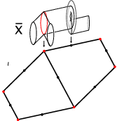
Now note that since for any 2-torus, the two curves along which the annuli are attached meet at a single point, the singular fibration has a section . Let denote the cone on . We now form the identification space obtained by attaching to along .
By construction, we have that the fundamental group of is precisely the right angled artin group associated to (simply choose the cone point of as the basepoint and for each vertex of let be the loop which runs from to , along the edge , around the circle associated to , and back along . Then one sees that the loops generate the fundamental group and the relations are precisely the commutator relations dictated by .)
We let denote the universal cover of and let denote the covering map. By denote . Given a torus in which is the fiber over the midpoint of an edge of , is a union of planes. Such planes are referred to as standard flats. For each edge of , let denote the annulus which is the closure of the union of fibers lying over the interior of . A component in of is called a standard strip.
We may obtain from by collapsing each annulus to a closed geodesic, and the cone on to a point; this defines a surjective piecewise linear map with contractible point inverses, and hence is a homotopy equivalence. Likewise we get a proper homotopy equivalence by collapsing the interval factor of each standard strip to a point, and collapsing each copy of in to a point.
Let denote the quotient of obtained by collapsing each standard flat to a point and each standard strip to an arc by projection onto the -factor. We refer to as the flat space associated to . All standard flats in are represented by points in , and we can think of as obtained from the (discrete) set of standard flats by connecting the dots in just the right way to obtain a very useful space (as we shall see).
Denote by the image of under the quotient map. There is an induced action of on ; let be the quotient map. Thus can be constructed from by collapsing the tori to points and collapsing the annuli to arcs, and therefore can be identified with the cone on . We will equip with the triangulation in which the base of the cone is the barycentric subdivision and is given the cone triangulation. Note that the image of in is the base of the cone. We will also equip with the triangulation obtained by pulling back via .
There are three types of vertices in :
- •
vertices of which are obtained from crushing flats to points are called flat vertices (in these correspond to the subdivision vertices in ),
- •
vertices of which are the cone points of copies of are called cone vertices, and
- •
the remaining vertices are called singular vertices; these are the vertices which correspond to the original vertices of
An arc joining two flat vertices which consists of two neighboring edges in is called an full edge of .
The action of on is simplicial, the stabilizers of flat vertices are isomorphic to , the stabilizers of the full edges are infinite cyclic, and . Thus this action endows with the structure of a (simple) complex of groups, in which the underlying complex is .
We endow and with a polyhedral metric as follows. Each torus fiber is given the structure of a flat square 2-torus, in which each of the designated curves along which fiber annuli are attached has length 1. The standard annuli are viewed as quotients of the unit square with a pair of opposite edges identified. Thus has the structure of locally square complex. Therefore, we just need to metrize the attached cone . Note that each 2-simplex in is of the form , where is the cone vertex, is the midpoint of an edge and is a vertex of . We endow such a simplex with the metric of an isosceles right triangle whose legs have length 1, so that the right angle is at the vertex . It is now easy to check that the space satisfies the condition (i.e. the links have no loops of length less than ). Note further that given an edge of , the cone on now consists of precisely two isosceles right triangles, forming a unit cube, so that in fact, has the structure of a locally square complex.
Consequently, is a square complex. Since is built out of copies of , we can similarly endow with the structure of a square complex (for a discussion of links see Observation 5.4 below). From now on, we will abuse notation slightly and refer to simply as or simply .
Theorem 5.1 (No flats in flat space).
The flat space is Gromov hyperbolic.
Proof.
Fix a small . Perturb the metric on by replacing each Euclidean triangle by a triangle with constant curvature whose angles are at , at and at . Since has no cycles of length it follows that this is a metric on which is quasi-isometric to the original metric. ∎
To summarize what we have done so far, we have the following.
Proposition 5.2.
The RAAG acts on by isometries and the following holds:
- (1)
has the structure of a square complex, with each square having two singular vertices, one flat vertex and one cone vertex.
- (2)
The quotient space is . We will denote the quotient map by . We lift the labeling of the vertices of (flat, cone, singular) to the vertices of via .
- (3)
There is a fundamental domain for the action of such that is a homeomorphism. We will identify .
- (4)
Stabilizers of flat vertices are .
- (5)
Stabilizers of singular vertices are .
- (6)
Stabilizers of cone vertices are trivial.
From the point of view of complexes of groups, we can say the following.
Observation 5.3.
- •
is an ordered simplicial complex (after adding cone-to-flat diagonals in all squares), with cone vertex initial, and flat vertices terminal (i.e. the edges are oriented from cone to singular to flat).
- •
, as an orbispace, is with the trivial label on the cone vertex, on the singular vertices, and on the flat vertices.
Observation 5.4.
- •
The link in of every cone vertex is .
- •
The link in of every flat vertex is (the join of two infinite countable sets of vertices) and the stabilizer is acting in the obvious way: translates one by 1 and fixes the other , and fixes the first and translates the second by 1. In particular, the complement of the set of all flat vertices in is connected.
- •
The link in of every singular vertex is the join where is the link of the image vertex in . The stabilizer fixes and translates . The link of in is .
Each singular vertex has two natural objects associated with it: the track and the singular star. We describe these below.
5.2. The singular star associated to a singular vertex
Fix a singular vertex . Consider its star in . By Observation 5.4, can be identified with the star of in (barycentrically subdivided) . Thus is the union of all edges with one vertex at and the other vertex flat. We call the singular star associated to . Recall that the parallel set of a geodesic line in a space is the union of all geodesic lines parallel to . The vertex represents a geodesic line in and its parallel set will be denoted by .
Observation 5.5.
Recall that is the quotient map. Then . Conversely, every parallel set in of a standard line (i.e. a line in a standard strip) arises in this way for a suitable singular vertex . Moreover, the parallel set is the union of flats and strips that coarsely contain the given standard line. Abstractly, a parallel set in is isomorphic to where is the universal cover of the 1-complex obtained from by wedging a circle to every vertex other than .
The image of a parallel set in under the quotient map will be referred to as a parallel set in (even though it is not the union of lines parallel to a fixed line). It is a subcomplex of , and the quotient by the stabilizer is .
Observation 5.6.
The intersection between and a nontrivial translate of it is contained in a singular star.
5.3. The track associated to a singular vertex
Again let be a singular vertex. Let be the edges that have one endpoint at and the other endpoint flat (thus the singular star is the union of the ’s). Then contains squares that have as a vertex. These squares can be enumerated so that is one of the sides of , . Note that by construction, these squares share a common edge that is incident to and whose other endpoint is the cone point, so that is distinct from the edges . Let be the hyperplane in transverse to ; this is well-defined since is a square complex, see Section 2.2. This is the track associated to .


Observation 5.7.
Recall that is the quotient map.
- •
is a collection of hyperplanes in . Each hyperplane is a convex subset of .
- •
Conversely, any hyperplane in is a component of for a suitable singular vertex .
Also denote by the closure of the component of that contains . Define the thickened track associated to to be
Observation 5.8.
- •
is a product neighborhood of , that is, .
- •
Let be a component of . Then contains a unique component of . Moreover, , where is the cone on with cone point .
- •
Under this identification, the pointwise stabilizer of acts on by fixing and the cone point, and translating the base of the cone.
Lemma 5.9.
- •
Every parallel set in separates . The set of complementary components is acted on freely and transitively by the subgroup fixing the parallel set pointwise.
- •
For any two distinct cone vertices in there is a parallel set that separates them.
Proof.
A parallel set has a product neighborhood as described in Observation 5.8. It follows from the simple connectivity of that the connected components of are in bijective correspondence with the connected components of ; the latter are in bijective correspondence with the subgroup fixing pointwise. For the second assertion, consider the geodesic joining the two vertices. This geodesic must cross some hyperplane, and hence some component of some (see Observation 5.7). The associated parallel set separates between the two cone vertices (see Observation 5.8). ∎
5.4. Coarse distance and parallel sets
We will be interested in paths and loops in ; these will correspond to sequences of standard flats in . There is a straighforward notion of distance between standard flats. Suppose that and are standard flats. The flats and correspond to two vertices in . Note that since is a bipartite graph, the usual path distance in between is even; let denote half this path distance in . We will be interested in a somewhat different notion of distance on , called coarse distance, which we now describe. We say that the coarse distance between and is 1, , if they coarsely intersect in a line, or equivalently, if belong to the same parallel set (cf. Lemma 2.2). We will say that , if their exists a sequence of standard flats such that and is the smallest number for which there exists such a sequence. Note that this then defines a metric on the set of flat vertices of . The reason this metric is natural is that it is preserved by quasi-isometries: the binary relation on of belonging to the same parallel set is quasi-isometry invariant, by Lemma 2.2 and Theorem 4.5.
The metric can be seen directly in as follows. Suppose that and are two full edges of meeting at a flat vertex . We say that and define a legal turn at if and have cyclic stabilizers with trivial intersection. Otherwise, they have the same cyclic stabilizer and we say that they define an illegal turn at . Now suppose that and are two flat vertices of . Suppose that is a full edge path in joining and . Then the coarse length of , is computed by counting the number of legal turns along and adding 1. Thus, the coarse distance between vertices is simply the minimal coarse length of a path between them.
If a path in has no legal turns in it, then in fact all the flat vertices along it correspond to flats which are all contained in the same parallel set. We call such a path a stalling path. The union of all stalling paths containing a given singular vertex is thus a parallel set in ; it corresponds in to the union of all flats and strips coarsely containing a given singular line.
6. Dual disk diagrams
We consider as a square complex. Let denote the union of hyperplanes in . We call a component of a block. Notice that each block contains a unique vertex of . Suppose that is a closed full edge path in . Then extends to a map . Now we may make transverse to the hyperplanes of . Thus is a union of embedded arcs and simple closed curves in , where each arc and closed curve is a component of the preimage of a single hyperplane. As in [Sag95], one may assume that there are in fact no simple closed curves and that each pair of arcs meets in at most a single point. Since is a 2-complex, we may further assume that there are no triangular regions: every collection of three arcs contains a disjoint pair. The pair is called a dual disk diagram for . Sometimes we will abuse notation and just refer to as the dual disk diagram. In [Sag95] it is shown that one can get from any diagram to any other through a sequence of triangular moves. Since there are no triangles, we see that the dual disk diagram is unique.
A region of refers to the closure of a component of . Note that each region is associated to a vertex of , namely the vertex whose block the region is mapped to. By a boundary region we mean a region that intersects . Regions that are not boundary regions are called internal regions. The union of all internal regions is called the core of the diagram. By a corner of we mean a triangular region bounded by two arcs of and a subarc of . A corner corresponds to running around the corner of a square of . Since is a path of full edges, this means that the corner of the square is a flat vertex and the turn at the vertex is a legal turn.
We now need to discuss some complications which can occur in general disk diagrams, but which will not appear in our setting, because our boundary map may be assumed to be an embedding.
6.1. Spurs
A spur of consists of a collection of nested arcs, each disjoint from all other arcs, so that one of the arcs has endpoints on neighboring boundary edges (this arc bounds a region with no curves or arcs in it) ; see figure below.
In this case, we see that the original full edge path has some backtracking. Since we will always be dealing with paths that have no backtracking, we can assume that there are no spurs.
![[Uncaptioned image]](0708.1937v1/spur.png)
6.2. Separating cells
Suppose that the intersection of a closed cell with the boundary of of has two distinct connected arc components , so that separates . Then the path represented by is not embedded. To see this, note that since is a path of full edges, and must each contain a vertex, and these vertices must map to the same vertex in . Because we will be dealing with embedded paths, we can assume that there are no separating cells.
The upshot of the above is that if the edge loop is embedded, then the disk diagram associated to it has no spurs or separating cells. An embedded full edge loop will be called a cycle.
Recall that there are three types of vertices: singular, flat, and cone vertices. Since each region of is mapped to a block, which is uniquely associated to a vertex of , we have three types of regions, which we also call singular, flat and cone regions.
Observation 6.1.
Every square in has two diagonally opposite singular vertices, one cone vertex and one flat vertex.
![[Uncaptioned image]](0708.1937v1/square.png)
Below is an example of a dual disk diagram. The yellow cells are the boundary cells and the remaining cells form the core.
![[Uncaptioned image]](0708.1937v1/diagram.png)
Observation 6.2.
Since corners cannot contain singular vertices, all corner regions are flat regions. Also, all cone regions are interior.
Observation 6.3.
Observation 6.1 can be transported to the disk diagram to tell us what types the regions are; around each intersection point of two arcs in the diagram, we have two diagonally opposite singular regions, one cone region and one flat region. In particular, this tells us that (under our standing assumption that our paths are embedded) the core is always not empty.
Observation 6.4.
If is an arc of the disk diagram, then by Observation 6.1, we see that the regions immediately to one side of alternate singular and cone regions, while the other side of alternate singular and flat vertices. The latter sequence of regions gives us a stalling path in . Thus the vertices associated to this sequence of regions all lie in the same parallel set.
6.3. Existence of 1-shells or 2-shells (by the seashore).
Following McCammond and Wise, we define a boundary region of a disk to be an -shell if it has internal edges. In the example above, the core of the diagram has four 2-shells. Since the core of the diagram is a C(4)-T(4) complex, we can apply Greendlinger’s lemma. We give a slightly different statement suited to our needs and we for the sake of completeness, we include a proof here (for deeper delvings into such results see [MW02]).
Lemma 6.5.
Let be a disk tiled by polygons in such a way that every interior vertex is incident to at least 4 polygons and so that each polygon has at least 4 sides. Then one of the following holds.
- (1)
(i.e. there is one 0-shell)
- (2)
there are at least two 1-shells
- (3)
there is at least one 1-shell and at least two 2-shells
- (4)
there are at least four 2-shells
Proof.
A corner of is an unordered pair of adjacent edges. Thus an -gon has corners (assuming ). We say that a corner of is contained in if the interiors of the corresponding two edges do not intersect any other ’s. Denote by the number of sides of and by the number of corners of contained in .
View each as a square complex with squares so that curvature is concentrated at one interior vertex. The excess angle at this vertex is . Thus the total interior excess is at least
(it might be larger if there are interior verices incident to polygons).
The boundary deficit is for each corner, i.e. at most
(it might be smaller if there are boundary vertices incident to polygons). Recall that Gauss-Bonnet says:
Thus
and hence
The statement now follows quickly. To each assign the score of points. The inequality says that the sum of all points is . If is assigned 4 points, it is a 0-shell. If it is assigned 2 points it is a 1-shell, and if it is assigned 1 point it is a 2-shell. (An interior triangle would get 1 point but we are assuming there are no triangles. All other polygons get a nonpositive number of points.) ∎
Remark 6.6.
Suppose that there are precisely two 1-shells and no 2-shells. Then the polygons can be renumbered so that and are 1-shells and and share an edge iff . In other words, the polygons form a ladder.
6.4. Shells, short cuts and taut cycles
A cycle is said to have an i-cut if there are flat vertices on such that the coarse length of any path along the cycle between and is greater than , but for which there exists full edge path of length in joining and . A cycle is said to be taut if there exists no -cut with .
Now suppose that is a disk diagram for and let be its core. If is not a single cell, then by Lemma 6.5, has a 1-shell or a 2-shell. As we see in the figure below, we then obtain a 1-cut or a 2-cut for .

Thus we obtain the following lemma.
Lemma 6.7.
(Diagrams for taut cycles) Suppose that is a taut cycle. Then the diagram for has a core consisting of a single cell.
7. Rigidity of taut cycles
The aim of this section is to prove the the quasi-isometric preservation of taut cycles. Recall that if is a quasi-isometry, Theorem 4.5 tells us that standard flats are coarsely preserved by . Since no two standard flats are coarsely equivalent, induces a bijection on the flat vertex set of . Moreover, since coarse equivalence is preserved by quasi-isometries, we have that is preserved.
Theorem 7.1 (Taut cycle rigidity).
Suppose that and are as above. Then carries taut cycles to taut cycles. In particular, full edges that lie along taut cycles are carried to full edges.
We first prove a lemma that tells us that “quasi” cuts of length at most 3 actually give 1-cuts or 2-cuts.
Lemma 7.2 (quasi-cuts yield cuts).
Let be a cycle. Suppose that there exist non-adjacent flat vertices and along , subdividing into two paths and . Suppose further that and are joined by a path so that
- (1)
- (2)
and are the only flat vertices of which lie in .
Then is not taut.
Proof.
We give the argument when . The argument when is similar and indeed simpler. So we suppose that is broken up by two flat vertices and into three stalling subpaths and as in Figure 5

We let denote a dual disk diagram for the loop . Note that by assumption, this loop is indeed a cycle. We will apply Lemma 6.5 to . Now we must consider some cases.
Case 1: and are both longer than 1. Since there are no corners along stalling sections of , it follows that is not a single cell so we are in cases 2,3, or 4 of Lemma 6.5. Now a shell gives at least two consecutive corners along . It follows that if a shell produces corners along , it is either a sequence of corners that begins at or and continues into or the sequence of corners is simply the pair of corners at and (in this case, is of length 1).
There exist 1-shells (case 2 or 3 of Lemma 6.5). Let us suppose we have a 1-shell in . Now a 1-shell produces a sequence of corners of length at least three, so it cannot occur at and . Also, both of the endpoints of the 1-cut produced by this shell cannot be along the non-stalling section of , for otherwise would not be taut. Thus, one of the endpoints of the 1-cut must be along the stalling sections or . But since these stalling section can only have a corner at and , the 1-cut provides a 2-cut between or and some vertex in the non-stalling section (see Figure 6). Thus is not taut and we are done.

There exist no 1-shells (case 4 of Lemma 6.5). In this case there are at least four 2-shells. Since only two of these can produce corners at the vertices and , and only one can produce corners at and , we must have a 2-shell which produces a 2-cut in the non-stalling section, namely along . This produces a 2-cut for and we are done.
Case 2: Only one of has length 1. Assume without loss of generality that has length 1, and is longer. We proceed as in Case 1. If there exist 1-shells, there are at least two 1-shells or a 1-shell and two 2-shells. It follows that one of them cannot be along . As before, these shells cannot occur entirely along . Thus we are in the case in which there are only two -shells, ; that is, we have two 1-shells. One of these must have its first corner at and we get a 2-cut as in Figure 6.
If we have only 2-shells, then there are 4 of them, and hence one of them must occur entirely along the , producing a 2-cut for , contradicting the tautness of .
Case 3: both and have length 1. Now if does not have a corner at both and , then we may proceed as before. So suppose that there are corners both at and . We now return to our original loop . Let be the flat vertex immediately adjacent to along and let be the flat vertex immediately adjacent to along . Let be the vertex along immediately adjacent to . We define and similarly as neighboring vertices of . Now since there is a corner at , it follows that the path is non-stalling. Thus, the path is a stalling path. Similarly, the path is a stalling path. ( See Figure 7.)

We thus let be the subarc of spanned by and , and let be . We then consider a dual disk diagram for and we are back in Case 1 with replaced by and replace by . ∎
Proof of Theorem 7.1.
Suppose that are the flat vertices along a taut cycle . Let . We know that , so that we can choose a full edge geodesic joining to , such that flat vertices along it lie in the same parallelism class. We then join the ’s together to get a closed loop . We claim that this loop is a cycle. First of all, by construction, the ’s are embedded, and at the ’s we have turns, so that there is no backtracking. Secondly, if distinct ’s met along a vertex which was not one of the endpoints, then we could apply Lemma 7.2 to conclude that is not taut. So now consider a dual disk diagram for for and as usual let denote the core of . We claim that consists of a single cell.
If has more than one cell, we would then have an arc in which separates into two regions, each of which contains a 1-shell or 2-shell of . Now by Observation 6.4, there would be a stalling path joining non-adjacent vertices and of . Now if we have and , for some , then we have that and we apply Lemma 7.2 to conclude that was not taut. Now if , then let be a closest such vertex to and be a closest such vertex to . Letting and . We see that the path satisfies the conditions of Lemma 7.2. We can apply Lemma 7.2 in a similar manner when only one of the ’s is in .
We thus have that consists of a single cell. This means that in fact the define a closed edge loop . Now we wish to show that this loop is taut. Suppose not. Then we have a 1-cut or a 2-cut of . Pulling such a cut back via gives a quasi-cut as in Lemma 7.2 thus implying that is not taut, a contradiction. ∎
8. -rigidity
We next need to argue that if are two standard flats in that intersect in a line, then their images intersect in a line as well. A priori, we only know that they intersect coarsely in a line, i.e. that they belong to the same parallel set. If there is a taut cycle that crosses both and then the fact that is a line follows from taut cycle rigidity. However, there are pairs of flats where there are no such taut cycles. This is of course the case if the graph contains valence 1 vertices, but there are no such vertices by our standing assumption on . For a more subtle failure see the example below.
8.1. Lemmas about graphs
Definition 8.1.
Let be an embedded cycle in the defining graph . An -shortcut is an edge-path in of length whose endpoints are in and whose distance in is .
Definition 8.2.
A cycle is tight if it does not admit any 1-shortcuts nor any 2-shortcuts.
Remark 8.3.
If is a cycle in , we can lift it to a cycle in the barycentric subdivision . Then is tight in iff is taut in .
Example 8.4.
Let be the atomic graph obtained from the 1-skeleton of a dodecahedron by doubling along one of the pentagons representing a face. Then every tight cycle is contained in one of the two copies of the dodecahedron, so that a pair of edges that share a common vertex but are not contained in the same dodecahedron give rise to flats that intersect but are not both crossed by a tight cycle.
Definition 8.5.
Let be a vertex of and the link of in . The Whitehead graph at is the graph whose vertex set is and (represented by edges with initial vertex ) are connected by an edge iff there is a tight cycle in that enters along and leaves along .
In the above example, the Whitehead graph at every valence 3 vertex is the complete graph (i.e. a triangle), while at the valence 4 vertices it is obtained from the complete graph by removing an edge (i.e. it is a square with one diagonal).
Lemma 8.6.
is connected iff is not a cut vertex.
Proof.
It is clear that is disconnected if is a cut vertex. For the converse, suppose is disconnected, and let be the vertices of one of the components of , and let be all the other vertices of . Suppose is not a cut vertex. Then there are embedded cycles in that enter along some and leave along some . Let be a shortest such cycle. We claim that is tight. To see this, suppose is an -shortcut for for . Using the fact that has no -cycle, it follows that one may replace a subpath of with to obtain a shorter cycle which contains some and some . Thus some is connected to some in , a contradiction. ∎
Lemma 8.7.
An atomic graph contains no cut vertices, or separating closed edges.
Proof.
Let be either a vertex or a closed edge, and suppose is a vertex. Note that if is a connected component, then cannot be contained in the the closed star of , because it would then lie in a single edge of , which clearly contradicts the assumption that every vertex has valence at least . ∎
Lemma 8.8.
Suppose the edges of an atomic graph are colored in three colors, black, white, and gray, and the following holds:
- (1)
any two gray edges share a vertex, and
- (2)
the edges of any tight cycle are either all black or gray, or they are all white or gray.
Then the edges of are either all black or gray, or else they are all white or gray.
Proof.
Suppose not. Thus there is an edge colored black, and there is an edge colored white. All gray edges have a vertex in common (by assumption (1) and because there are no triangles). Let be the union of all (closed) gray edges. We now claim that does not separate . Indeed, take . If then can be joined by a path missing and hence missing . Say . If is a vertex, then it is adjacent to and it is incident to an edge different from (since otherwise would be a separating edge). Thus can be joined by a path in the complement of to the complement of . If is not a vertex, then it is an interior point of some edge and it can again be joined by a path in the complement of , first to and then to the complement of as before. Similar considerations apply to and our claim is proved.
Now join and by a path missing . Thus all edges along this path are black or white, and there is a vertex along this path where color changes from black to white. Therefore all edges incident to are black or white and at least one is black and at least one is white. By Lemma 8.6 there is a tight cycle passing through and at crossing one white and one black edge. But this contradicts our assumption (2). ∎
Lemma 8.9.
Let be graphs with no vertices of valence and no cycles of length . Suppose is a bijection of the sets of edges of , such that
- •
if share a vertex then share a vertex.
Then there is a graph isomorphism that induces .
Proof.
Let be a vertex of . Consider the set of all edges in that contain . By our assumptions on , and any two of the edges share a vertex. Since has no cycles of length it follows that there is a unique vertex contained in all . Define . By construction, if span an edge then span an edge. Thus is a simplicial map. Reversing the roles of provides a simplicial map and it easy to see that and are identity. ∎
8.2. -rigidity
The following is the main theorem in the paper. It says that the flat space is a quasi-isometry invariant of the RAAG . The notation should be self-explanatory, e.g. .
Theorem 8.10.
Let be two atomic graphs. Let be a quasi-isometry between the associated RAAGs. Then there is a label-preserving isometry between the associated flat spaces such that for each standard flat (i.e. a flat vertex) we have that is contained in a Hausdorff neighborhood of the flat .
In particular, takes each cone in isometrically to a cone in , and .
Proof.
By Theorem 4.5 we have a function defined on the set of flat vertices and satisfying the statement about the Hausdorff neighborhood. This map is a bijection. We now extend this map to an isometry.
Step 1. Let be the fundamental domain (see Proposition 5.2(2)). We claim that takes all flat vertices in into a translate of the fundamental domain . By Theorem 7.1 we know that sends all flat vertices along a taut cycle in into a single cone (and this cone is unique, see Observation 5.6). Since every flat vertex in lies along a taut cycle it suffices to prove that there is a cone that contains the images of the flat vertices along any taut cycle in .
So suppose this is not true, and that for two different taut cycles in the images of the flat vertices are contained in different cones . Choose a parallel set that separates between and (see Lemma 5.9) so that we can write with , and . Now color the edges (i.e. the flat vertices) of into black, white or gray according to whether they are mapped into , or . Note that any two gray edges share a vertex (the corresponding flats coarsely intersect in a line; for edges of this happens only when the edges share a vertex). Now by Lemma 8.8 we see that all flat vertices in are mapped to either or to contradicting our choices.
Thus, after composing with an element of , we may assume that maps the flat vertices in to flat vertices in . By considering the inverse map, restricts to a bijection between the sets of edges of and .
This analysis can be applied to any translate of . As a result of Step 1, we can extend to the cone vertices so that it induces a bijection between the sets of cone vertices and any adjacent pair of a flat and a cone vertex maps to an adjacent pair.
Step 2. Now consider restricted to the “base of the cone”, that is, the map . Apply Lemma 8.9 to deduce that extends to an isomorphism . Adjacent edges map to adjacent edges since only in this situation the corresponding flats coarsely intersect in a line, so the lemma applies.
Step 3. It remains to extend to the singular vertices. Let be a singular vertex, say in . Then there is a unique way to define so that preserves adjacency with the flat vertices in (this is Step 2). We need to verify that when we regard as a vertex in a different cone we obtain the same . There are cones that contain (see Proposition 5.2) and all these cones also contain all flat vertices adjacent to , so the claim follows. ∎
9. The proofs of corollaries 1.7, 1.8, and 1.9
Proof of Corollary 1.7. Suppose and are atomic graphs, and is a quasi-isometry. Let be the bijection provided by Theorem 1.6. Pick and let . Then establishes a bijection between the standard geodesics (respectively standard flats) passing through and the standard geodesics (respectively standard flats) passing through . This induces an isomorphism of the defining graphs. ∎
Proof of Corollary 1.8. Let be an isomorphism. Then we obtain an isometric action , which is discrete and cocompact. Hence by the fundamental lemma of geometric group theory, there is a -equivariant quasi-isometry
Let be the bijection furnished by Theorem 1.6.
Consider a standard flat . By Theorem 1.6, there is a standard flat such that maps bijectively to , and respects the product structures. Since is equivariant with respect to the stabilizer of , it follows that the induced mappings and are also -equivariant. Since acts transitively on , , , and , the map is the restriction of an isometry . Hence is the restriction of an isometry . ∎
Proof of Corollary 1.9. Let be a homotopy equivalence. Then induces an isomorphism and we may lift to a quasi-isometry
which is -equivariant (where we identify and using the isomorphism above). By Corollary 1.8 there is a -equivariant isometry at bounded distance from , and this descends to an isometry
which is homotopic to .
∎
10. Further implications of Theorem 1.6
At first sight, one might think that the map in the conclusion of Theorem 1.6 must be the restriction of an isometry, since it preserves so much structure; however, this turns out not to be the case. In this section we single out part of the structure of the bijection which efficiently distinguishes between quasi-isometries, namely we associate with each parallel set a biLipschitz homeomorphism of a copy of the integers. In the next section we will see that any biLipschitz homeomorphism can arise this way.
Let be a quasi-isometry, where and are associated with atomic RAAG’s, and let be the map of Theorem 1.6.
Let and denote the collections of maximal standard product subcomplexes in and , respectively. Since and are atomic, each or is the parallel set for a standard geodesic. Therefore splits isometrically as a product of complexes .
Definition 10.1.
For each parallel set , we define to be the -factor in the splitting
and let to be the set of vertices of , equipped with the induced metric.
Lemma 10.2.
For every there is a such that maps bijectively to , preserving the product structure.
Proof.
Let be a standard geodesic parallel to the -factor of . Then Theorem 1.6 implies that is mapped bijectively by to , for some standard geodesic . Since any two geodesics , obtained this way are parallel, it follows that is contained in a parallel set. Applying the same reasoning to the inverse implies that for some .
Since preserves standard geodesics, it follows that preserves product structure. ∎
By abuse of notation we use to denote the induced bijection given by Lemma 10.2. By the lemma, for each , we obtain a bijective quasi-isometry , where the quasi-isometry constants are controlled by those of .
Lemma 10.3.
- (1)
If is an isometry, then is an isometry for every .
- (2)
If is induced by an element of the commensurator , then for every , the map is equivariant with respect to cocompact isometric actions on and .
Proof.
Assertion (1) is immediate.
There is an isomorphism where and are finite index subgroups, such that is -equivariant, where acts freely, cocompactly, and isometrically on via the isomorphism . Then is also -equivariant. Hence if stabilizes , then it also stabilizes the parallel set . In other words, the map restricts to a -equivariant mapping . Since acts cocompactly on , assertion (2) follows. ∎
11. Quasi-isometric flexibility and the proof of Theorem 1.10
The homomorphism is injective. Suppose . By Corollary 1.8 there is an isometry which induces , i.e. we identify with a subgroup of . If , then commutes with a finite index subgroup of , and therefore has bounded displacement,
If follows that maps each standard flat to itself. Since the intersection of the standard flats passing through a vertex is precisely , it follows that fixes every vertex, and is therefore the identity map.
The homomorphism is injective. Suppose . Then can be represented by an isomorphism , where the ’s are finite index subgroups of . Therefore there is a quasi-isometry which is -equivariant, where we identify with via , and use the corresponding action on the second copy of . If , then is at bounded distance from the identity. Letting be the bijection given by Theorem 1.6, we may argue as in the preceding paragraph to conclude that . It follows that .
has infinite index in . Pick a vertex , and a positive integer . Let be the homomorphism which sends the generator to , and the other generators to . Let be the kernel of , and be the -fold cover of given by . One may describe as follows. Begin with , which is a product , where is a bouquet of -circles, where is the number of vertices adjacent to . To obtain from , one glues on a copy of , where is the graph obtained by deleting and the edges incident to . To obtain , one first passes to the -fold cyclic cover of , and then glues on -copies of .
Let be the graph obtained by taking copies of , and gluing them together along the copies of . In fact is homotopy equivalent to ; to see this, map to by taking of the copies of and collapsing them to copies of (by collapsing the interval factors). In particular, is isomorphic to the RAAG . Since is not atomic, this shows that the atomic condition is not commensurability invariant among RAAG’s.
Note that the permutation group of the set acts isometrically on by permuting the copies of , and hence we get a homomorphism . For each element , we may lift the corresponding homotopy equivalence to a quasi-isometry which preserves a parallel set covering . Moreover, the induced map will be equivariant with respect to the action of on by translations, and descends to the permutation of corresponding to .
Now consider the collection of elements obtained this way, as varies over the positive integers, and varies over the permutation group of . If had finite index in , we could finite a finite collection such that for each there is a such that for some . This means that , and that
agrees with . However, by part 1 of Lemma 10.3, is an isometry. This clearly contradicts the fact that can come from any permutation of , for any .
Remark 11.1.
Let denote the group of isometries of covering the permutation action . Then there is a short exact sequence
Thus is commensurable with . However, there is no geometric action of on . This can be deduced by examining the subgroup of which stabilizes a parallel set , and observing that the induced action on is not conjugate to an isometric action.
has infinite index in . The construction is similar to the proof that .
Pick , and look at the infinite cyclic cover corresponding to the homomorphism which sends to and the other generators to . Then can be obtained from by gluing on infinitely many copies of . As in the preceding paragraphs, we may produce homotopy equivalences by “permuting the copies of ”. By lifting these homotopy equivalences we may obtain quasi-isometries which preserve a parallel set covering , and hence obtain a bijective quasi-isometry . It is not hard to see that any bijective quasi-isometry may be obtained in this way.
If were finite, there would only be finitely many possibilities for the ’s up to pre-composition by maps of the form , where comes from an element of the commensurator. In view of Lemma 10.3, this is clearly not the case.
References
- [Ahl02] A. R. Ahlin. The large scale geometry of products of trees. Geom. Dedicata, 92:179–184, 2002. Dedicated to John Stallings on the occasion of his 65th birthday.
- [Bas72] H. Bass. The degree of polynomial growth of finitely generated nilpotent groups. Proc. London Math. Soc. (3), 25:603–614, 1972.
- [BKS07] M. Bestvina, B. Kleiner, and M. Sageev. Quasiflats in -complexes. Preprint, 2007.
- [BM00] M. Burger and S. Mozes. Lattices in product of trees. Inst. Hautes Études Sci. Publ. Math., (92):151–194 (2001), 2000.
- [BN06] J. Behrstock and W. Neumann. Quasi-isometric classification of graph manifold groups. math.GT/0604042, 2006.
- [CCV] R. Charney, J. Crisp, and K. Vogtmann. Automorphisms of two-dimensional right-angled artin groups. math.GR/0610980.
- [CD95] Ruth Charney and Michael W. Davis. The -problem for hyperplane complements associated to infinite reflection groups. J. Amer. Math. Soc., 8(3):597–627, 1995.
- [Cha] Ruth Charney. An introduction to right angled Artin groups. arXiv, math.GR/0610668.
- [Dav98] Michael W. Davis. Buildings are . In Geometry and cohomology in group theory (Durham, 1994), volume 252 of London Math. Soc. Lecture Note Ser., pages 108–123. Cambridge Univ. Press, Cambridge, 1998.
- [Dro87] Carl Droms. Isomorphisms of graph groups. Proc. Amer. Math. Soc., 100(3):407–408, 1987.
- [Dun85] M. J. Dunwoody. The accessibility of finitely presented groups. Invent. Math., 81(3):449–457, 1985.
- [Gro81] M. Gromov. Groups of polynomial growth and expanding maps. Inst. Hautes Études Sci. Publ. Math., (53):53–73, 1981.
- [Gro87] M. Gromov. Hyperbolic groups. In “Essays in group theory”, pages 75–263. Springer, New York, 1987.
- [Gro93] M. Gromov. Asymptotic invariants of infinite groups. In Geometric group theory, Vol. 2 (Sussex, 1991), volume 182 of London Math. Soc. Lecture Note Ser., pages 1–295. Cambridge Univ. Press, Cambridge, 1993.
- [HM96] Jens Harlander and Holger Meinert. Higher generation subgroup sets and the virtual cohomological dimension of graph products of finite groups. J. London Math. Soc. (2), 53(1):99–117, 1996.
- [JŚ01] Tadeusz Januszkiewicz and Jacek Świa̧tkowski. Commensurability of graph products. Algebr. Geom. Topol., 1:587–603 (electronic), 2001.
- [KKL98] M. Kapovich, B. Kleiner, and B. Leeb. Quasi-isometries and the de Rham decomposition. Topology, 37(6):1193–1211, 1998.
- [KL97] M. Kapovich and B. Leeb. Quasi-isometries preserve the geometric decomposition of Haken manifolds. Invent. Math., 128(2):393–416, 1997.
- [KL07] B. Kleiner and B. Leeb. Induced quasi-actions: a remark. preprint, 2007.
- [KMLNR80] K. H. Kim, L. Makar-Limanov, J. Neggers, and F. W. Roush. Graph algebras. J. Algebra, 64(1):46–51, 1980.
- [KPS73] A. Karrass, A. Pietrowski, and D. Solitar. Finite and infinite cyclic extensions of free groups. J. Austral. Math. Soc., 16:458–466, 1973. Collection of articles dedicated to the memory of Hanna Neumann, IV.
- [Lau95] M. R. Laurence. A generating set for the automorphism group of a graph group. J. London Math. Soc. (2), 52(2):318–334, 1995.
- [MSW03] L. Mosher, M. Sageev, and K. Whyte. Quasi-actions on trees. I. Bounded valence. Ann. of Math. (2), 158(1):115–164, 2003.
- [MW02] Jonathan P. McCammond and Daniel T. Wise. Fans and ladders in small cancellation theory. Proc. London Math. Soc. (3), 84(3):599–644, 2002.
- [Sag95] Michah Sageev. Ends of group pairs and non-positively curved cube complexes. Proc. London Math. Soc. (3), 71(3):585–617, 1995.
- [Ser89] Herman Servatius. Automorphisms of graph groups. J. Algebra, 126(1):34–60, 1989.
- [Sta68] J. R. Stallings. On torsion-free groups with infinitely many ends. Ann. of Math. (2), 88:312–334, 1968.
- [Wis96] D. Wise. Non-positively curved squared complexes, aperiodic tilings, and non-residually finite groups. Princeton thesis, 1996.