Zero temperature conductance of parallel T-shape double quantum dots
Abstract
We analyze the zero temperature conductance of a parallel T-shaped double quantum dot system. We present an analytical expression for the conductance of the system in terms of the total number of electrons in both quantum dots. Our results confirm that the system’s conductance is strongly influenced by the dot which is not directly connected to the leads. We discuss our results in connection with similar results reported in the literature.
pacs
73.63.Kv; 73.23.-b; 72.15.QmI Introduction
Recent advances in the fabrication and precise control of nanoscale electronic systems lead to an increased interest in the study of many body effects in quantum dot structures. The Anderson single impurity model anderson was extensively explored to successfully understand electronic correlations in small single, or double quantum dot structures. In general, single or double quantum dot configurations provide the ideal systems to study many body effects. For example, single dot configurations allow the realization of the Kondo regime of the Anderson impurity singledot. On the other hand, double quantum dot (DQD) configurations provide the ideal candidate for the study of the many body effects associated to both Kondo effect and RKKY interaction doubledots. The connection of several quantum dots (QD) gives rise to remarkable phenomena due to the interplay of electron correlations and interference effects which depend on how the dots are arranged. One possible configuration is the double quantum–dot (DQD) system, where the dots are connected to the same leads and between them. Recently, Dias da Silva et al. 1 studied a DQD with one dot in the Kondo regime and the other close to the resonance with the connecting leads. One of the most interesting results reported in Ref. 1 is the finite temperature analysis of the parallel T-shape double dot configuration with one dot disconnected from the leads (Fig. 1) using the idea of interference between resonances. In such a configuration, the active dot A is directly connected to the left and right leads and to a side dot S. They showed that when the side dot S is coupled to the leads only through the active dot A, the Kondo resonance from the side dot S develops a sizable splitting even if there is no magnetic field in the system. This band filtering produced by the connected dot preserves the Kondo singlet and at finite temperature the magnetic moment is completely screened.
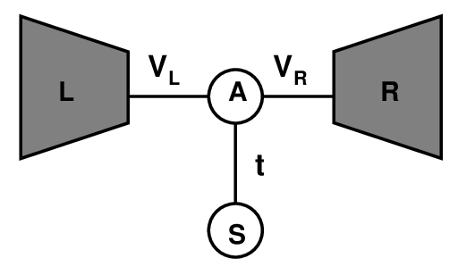
The calculation of system’s conductance is of major interest both for single and double quantum dots configurations. For double quantum dot configurations the problem was considered extensively using different methods, however, the results presented by different authors are in agreement only partially kim; tak; co; zi. The system’s electronic conductance is realized through the active dot A, however, the presence of the side dot S will influence the total conductance of the parallel T–shaped quantum dot system kim. The suppression of the system’s conductance at low temperatures can be understood if two possible conduction paths are considered, a direct path through the active dot A () and an indirect path through the side dot S (). New features have been pointed out by Takazawa et al. tak in connection with the inter–dot coupling strength and the values of the energies of the active dot and the energy of the side dot . For the case the occurrence of a non trivial suppression of the conductance was associated with a Fano–like effect between two distinct channels, i.e., the direct Kondo resonance of the active dot A and the indirect resonance via both the active and side dots. An interesting feature of the system was discussed by Cornaglia and Grempel co and by Zitko and Bonca zi using the new idea introduced in Ref. wiel known as the two-stage Kondo effect, a behavior obtained for a dot in a strong magnetic field. The T–shape DQD close to half–filling has a similar behavior for small inter–dot coupling , the possibility of a two-stage Kondo effect leading to a nonmonotonic behavior of the conductance as function of the gate voltage and magnetic field. At large inter–dot coupling the magnetic moments of the two quantum dots form a “local” molecular spin–singlet and the conductance varies monotonically at low temperature. One of the main results from co is the calculation of the conductance in terms of the spectral density of the active dot A interacting with the side dot S. The zero temperature conductivity depends on the total number of electrons in the two dots, i.e., the active dot A and the side dot S.
Here, we present a K calculation for the dc conductance of the T-shaped quantum dot system. Our analysis will start from a general Hamiltonian describing the possible interactions in the double quantum dot system, i.e., interactions inside each component dot, inter–dot interactions, and interactions with the reservoirs. Previous results obtained by Cornaglia and Gempel co give the system’s conductance in terms of the total electron density in the system. However, as we will prove later in the paper, there are additional contributions related to the inter–dot electron–electron interaction which were not included in Ref. co. We will also consider the system’s conductance in the presence of a magnetic field whose role is to remove the spin degeneracy for the possible bound states in the active and side dots. All our calculations are performed in the K limit, so finite temperature effects will be neglected. The relevance of temperature effects due to the different Kondo regimes can be evaluated by calculating the self energies of the electrons using the equation of motion method with an appropriate decoupling, however, the finite temperature conductance of the system will be the subject of another investigation cris.
II The Model
The general hamiltonian of the T–shape double quantum dot configuration is
| (1) |
Here, describes both the active A and side S dots
| (2) | |||||
where represents the on–site electron–electron Coulomb interaction and describes the coupling between the active and side dots. The operators and () are the standard electron creation and annihilation operators. The electrons in the left (L) and right (R) electrodes are described by
| (3) |
where the index ; () creates (annihilates) an electron with momentum and spin in the electrode of the configuration. The coupling between the T–shape DQD and the leads is described by the Hamiltonian which has the form:
| (4) |
All the properties of T-shape DQD configuration can be obtained from the Green function of the –electrons. The –electron’s Green function can be obtained by different methods including the equation of motion method (EOM) or the perturbation theory. In the following we will explore the EOM to extract the electronic Green function and thereafter the configuration’s total conductance.
The properties of the T-shape DQD can be expressed in terms of a Green-function matrix according to the Dyson equation
| (5) |
where is the noninteracting Green function
| (6) |
with and is the self–energy matrix as it results from the Coulomb electron–electron interactions, . In the most general form the self–energy matrix can be written as
| (7) |
a form which accounts both for electron–electron interactions in each of the two dots and for electron–electron interactions between the two dots of the configuration. The exact Green’s function and the self–energy of the system satisfy the Luttinger theorem:
| (8) |
where represents the trace of the matrix. The knowledge of the electronic Green’s function permits the calculation of the total electron density in the system as:
| (9) |
The above expression can be simplified to
| (10) |
III Conductance
Confinement of electronic systems in small quantum dot configurations may result in very interesting transport properties. Here, we calculate the T-shape DQD system’s transport properties following the general formalism introduced by Meir and Wingreen meir. According to Ref. meir the current through a quantum dot system in the presence of an external bias voltage is given by
| (11) | |||||
where represents the Fermi–Dirac distribution function, and
| (12) |
In the zero temperature limit, K, we can evaluate the conductance of the T-shape DQD configuration () as
| (13) |
where . The calculation of the system’s conductance as function of the total number of electrons () is relatively simple, and a general formula can be given as
| (14) |
where and are the renormalized energies of the bound states in the active, respectively side, quantum dots of the configuration. Eq. (14) is an exact result which shows that the dc conductance of the system depends on two coupling parameters, - the coupling between the active and side dots and - the coupling between the active dot and the leads, and the value of the system’s self–energy. Accordingly, the behavior of the system’s conductance depends on the selection of the constituent dots and on the external applied bias. For example, in Figure 2 we plotted the value of the relative conductance, , as function of the relative inter dot coupling for various values of the relative energy level of the side dot and a fixed value of the relative energy level in the active dot. Such graphic representations of the T-shape DQD conductance as function of various interaction energies in the system allow the optimal selection of the active and side dots. Our plotting assumes fixed values for the energy levels inside the active and side dot. This assumption may be questionable as for many-body effects in the system the initial energy of the bound states in the two component dots will be changed; however, in most of the real situations the corrections due to the self-energy on the value of the two bound states, and , are small, and in a first approximation they can be neglected. Tsvelik and Wiegmann calculated the self-energy due to the Coulomb interaction tsvelik and proved that the real part of the self-energy depends linearly on frequency . At , in the Fermi liquid approximation, the main contribution to the self-energy comes from the term and accordingly it can be neglected.

On the other hand Eq. (10) gives a direct relation between the system’s self energy and the total number of electrons in the constituent dots. As a result, the conductance of the T-shape DQD system can be expressed also using the total number of electrons in the active and side dots. A straightforward calculation, which implies Eqs. (10) and (14), gives
| (15) |
and in terms of the total number of electrons the system’s conductivity becomes
| (16) |
Note that depends also on the system’s self-energy, and implicitly on the total number of electrons in the system. However, for the side dot, which is not directly connected to the leads, the changed of the bound state energy is much smaller that for the active dot, and such a dependence can be neglected. Eq. (16) is an exact result which describe the dependence of the system’s dc conductance on the total number of conduction electrons. From the experimental point of view the total number of electrons in the system is controlled using the applied external bias.
In the absence of an external magnetic field, when the two considered dots are unpolarized (=) the normalized conductance can be written as
| (17) |
where is the total number of electrons in the active and side dots. It is easy to see that the zero temperature conductance of the T-shape DQD system vanishes when the total number of available electrons in the active and side dots is even. This result was already predicted in Ref. co. Our calculation for the system’s conductance also accounts for the intra and inter dots electron–electron interactions. For a finite occupancy of the T-shape DQD system, i.e., integer number of electrons occupy the two possible energy levels, the correction term will cancel ( for -integer). However, this fact is not an indication that the electron-electron interactions in the system can be neglected, the available number of electrons on the active and side dots being strongly dependent on these interactions and on the applied, external bias.
A different situation occurs when the degeneracy of the active and side quantum dots is removed. For example, when a small magnetic field is applied, the T-shape DQD becomes polarized and the possible energy levels become spin dependent. In this case, the system’s dc conductance becomes
| (18) | |||||
where represents the system’s magnetization. For any even number of electrons in the system (, , and ), the magnetization value reduces to the one presented in Ref. co for the case, i.e., . On the other hand, when the number of electrons in the system is odd, a different behavior of the magnetization should be expected, i.e., . Once again, the interaction term in the conductance will vanish for an integer number of electrons in the system.
IV Discussions
In this work we analyzed the conductance of a T-shape DQD. Our main result is a generalization of the unitary rule of the single-level Anderson impurity problem for the case of a T-shape DQD . The system’s conductance depends on various interactions inside the component dots, and on the value of the energy levels in the active and side dots. Tuning these interactions allow a direct control of the system conductance. We also presented a calculation of the system conductance in terms of the occupancy of the two possible energy levels in the active and side dots. A similar calculation was also presented in Ref. co, however, our result includes contributions related to the inter-dot interaction, . In the limit we recover the result presented in Ref. co. Additionally, we proved that such a term can be disregarded when the energy levels in the T-shape DQD system are occupied by an integer number of electrons. On the other hand, even at K or at small, but finite temperatures, when fluctuations are important, the occupancy of the energy levels can be non-integer, and in such situations the interaction correction to the system’s conductance becomes important. The differences between our calculation and the one presented in Ref. co are a consequence of how the general current passing through the system was calculated. The result presented by Cornaglia and Grempel co only accounts for the electron density in the active dot, and accordingly the conductance is calculated considering the inter-dot interaction small, the system behaving like a single dot with an electron occupancy . Such a result will be valid only in the limit .
Sweeping the gate voltage into and trough an odd valley in this model, corresponds to sweeping the energy of the active dot from above to below in the course of which the total number of electrons changes smoothly from to . We can obtain three different regimes for the system as function of various interaction parameters: (i) the “empty-orbital” when and ; (ii) the “mixed-valence” in which the number of electrons begin to increase due to strong charge fluctuations; and (iii) the “local moment” regime, in which the number of electrons approaches 1 and the local levels acts like a local spin in one of the dots, or in both. The latter regime can give rise to Kondo correlations, and the system has to be studied at finite temperature.
Our calculation is done in the K limit, however it may be extended to finite temperatures, K. In this limit, the imaginary part of the self-energy
| (19) |
when = and the real part of the self-energy is constant. The temperature scale, , is set by the Kondo effect and for the active dot can be calculated following the method proposed in Ref. kas.
The T-shape DQD system is a very promising quantum dot configuration, both from the fundamental physics and possible applications point of view. Systems involving single or multiple quantum dots may provide many opportunities for strong interaction effects studies. Also they may provide the optimal environment for the study of the Kondo effect, or of the Ruderman-Kittel-Kasuya-Yoshida interaction among local spins. Different other finite temperatures regimes can be considered by calculating the electronic self-energy using the equation of motion along with an appropriate decoupling cris.
References
- (1) P.W. Anderson, Phys. Rev. 124 (1961) 41.
- (2) S.M. Cronenwett, T.H. Oosterkamp , and L.P. Kouwenhoven, Science 281 (1998) 540.
- (3) N.J. Craig, J.M. Taylor, E.A. Lester, C.M. Marcus, M.P. Hanson, and A.C. Gossard, Science 304 (2004) 565.
- (4) L.G.G.V. Dias da Silva, N.P. Sandler, K. Ingersent, and S.E. Uolla, Phys. Rev. Lett. 97 (2006) 096603.
- (5) T.–S. Kim and S. Hershfield, Phys. Rev. 63 (2001) 245326.
- (6) K. Takazawa, Y. Imai, and N. Kawkami, J. Phys. Soc. Japan. 71 (2002) 2234.
- (7) P.S. Cornaglia and D.R. Grempel, Phys. Rev. B 71 (2005) 075305.
- (8) R. Zitko and J. Bonca, Phys. Rev. B 74 (2006) 045312.
- (9) W.G. van der Wiel, S. De Franceschi, J.M. Elzerman, S. Tarucha, L.P. Kouwenhowen, J. Motohisa, F. Nakajima, and T. Fukumi, Phys. Rev. Lett. 88 (2002) 126803.
- (10) Y. Meir and N.S. Wingreen, Phys. Rev. Lett. 68 (1992) 2512.
- (11) V. Kaschcheyevs, A. Aharony, and O. Entin–Wolman , Phys. Rev. 73 (2006) 125338.
- (12) M. Crisan, I. Grosu, and I. Ţifrea (in preparation).
- (13) A. M. Tsvelik and P. G. Wiegmann, Adv. Phys 32, 453 (1983).