Bound on the anomalous coupling from two-loop contribution to neutron electric dipole moment
Abstract
The two-loop contribution to the electric dipole moment (EDM) and the chromo electric dipole moment (CEDM) of an arbitrary fermion induced by the most general renormalizable coupling with complex left- and right-handed components ( and ) is calculated. The analytical expressions are numerically evaluated and the current experimental constraints on the electron, neutron and mercury atom EDMs are used to obtain a bound on the complex phase . It is found that the most stringent constraint, , arises from the neutron EDM.
, , ,
Although there is experimental evidence of CP violation, its origin still remains a mystery. In the standard model (SM), the only source of CP violation is the Cabbibo-Kobayashi-Maskawa (CKM) phase, which appears to be the origin of the CP violating phenomena observed in nondiagonal processes involving the and mesons [1]. On the other hand, as diverse studies had suggested [2], the CKM phase has a rather marginal impact on flavor-diagonal processes, such as the electric dipole moment (EDM) of elementary particles. For instance, the EDM of fermions arises up to three loops within the SM [3], thereby being extremely suppressed. It can be significantly enhanced, however, in several SM theoretical extensions, in which it can be induced at lower orders via new sources of CP violation. It means that any experimental signal associated with an EDM would point to new physics. Therefore, the EDM of light fermions, such as the electron and neutron, has been the subject of considerable interest in theories beyond the SM, such as supersymmetric models [4], multi-Higgs models [5], left-right symmetric models [6], and other theories [7]. Along these lines, a potential source of CP violation may be the coupling, whose study will be a top priority at the CERN large hadron collider (LHC). Such CP-violating effects would be induced via a complex phase arising from the simultaneous presence of both left- and right-handed components in the vertex, a scenario which is predicted indeed in several SM extensions. The purpose of this work is to calculate the two-loop contribution of the coupling to the EDM of a fermion. Although we will obtain a result valid for any charged fermion, our main goal is to use the experimental limits on the EDM of the electron and the neutron to constrain the complex phase associated with the anomalous vertex. As a byproduct, we will obtain the chromo electric dipole moment (CEDM) of and use the current experimental bound on the EDM of the mercury atom to constrain the anomalous part of the vertex.
The most general renormalizable coupling is given by the following Lagrangian
| (1) |
where are the usual left- and right-handed projectors and are unknown complex coefficients. The contribution to the on-shell vertex, which defines the electromagnetic properties of the fermion , is given, in the unitary gauge, via the Feynman diagrams shown in Fig. 1. Similar diagrams, with the photon replaced by a gluon, give rise to the CEDM. We will present the calculation of the vertex and then generalize the result to the coupling.
From the amplitude for the on-shell vertex we can obtain the EDM of , which is the term proportional to the Lorentz tensor structure . We will use the Feynman parameter technique to integrate over the arbitrary internal momenta. For the sake of completeness, we will present the most relevant details of the two-loop calculation in appendix A.

After solving the four-dimensional integrals arising from Fig. 1, the EDM of can be expressed as follows
| (2) |
where , is a quark color factor, and stands for the quadruple integral given in appendix A [Eq. (44)], which must be numerically evaluated in the most general scenario, namely, for internal and external fermions with non-negligible masses. On the other hand, in the approximation, which is suited for the purpose of our work as we are interested in evaluating the EDM of very light fermions, the parametric integral adopts the more simple form given in Eq. (46), which can be simplified further after some algebra:
| (3) |
with
| (4) |
It is not possible to integrate the function in terms of elementary functions, but it is straightforward to obtain a numerical solution due to the fact that is well-behaved in the corresponding domain.
It is useful to express the numerical value of the EDM and the the CEDM for a light fermion. Inserting the approximate value of the integral , we obtain for a very light fermion:
| (5) |
As for the CEDM of , , it follows easily from the above results. We just need to make the following replacements . Numerical evaluation gives:
| (6) |
We turn to analyze our results in the light of the current experimental limits on the EDM of fermions. Let be the experimental limit of the EDM of a fermion , which is not necessarily a light one. Then, our theoretical result for can be translated into the following bound on the complex phase:
| (7) |
This expression is exact as long as Eq. (46) is used for the parametric integral . In the case of a light fermion, we can use the result of Eq. (5).
We are now ready to constrain the phase . For this purpose, we will use the experimental data on the EDM of the electron, the neutron and the mercury atom.
The current experimental limit on the EDM of the electron is [8]:
| (8) |
Using this limit, we obtain the following bound
| (9) |
As far as the neutron is concerned, there are three different approaches to estimate its EDM [2]. In the chiral Lagrangian approach, is expressed in terms of the quark CEDMs, whereas in the QCD sum rule approach it is expressed as a combination of both quark EDMs and CEDMs. Due to the large discrepancies arising from these two approaches, it is convenient for the purpose of this work to estimate the neutron EDM using the non-relativistic quark model along with naive dimensional analysis for the quark CEDM contributions. In this approach, we have
| (10) |
where
| (11) |
with and being the respective QCD correction factor from renormalization group evolution. The CEDM contributions should be included as long as they are of similar size to those from the EDMs, otherwise they can be neglected. In our case, the quark CEDM is of similar size of the EDM, but its contribution to Eq. (11) is suppressed by more of one order of magnitude due to the factor . It is thus safe to neglect the CEDM contribution. On the other hand, currently the most stringent bound on the neutron EDM is [9]:
| (12) |
As usual, we take , with the neutron mass. The above Eqs. leads to a stronger bound than the one found from the electron EDM:
| (13) |
As for constrains on the EDM of diamagnetic atoms, the most stringent one can be obtained from the mercury atom. A constraint on the can be found following the approach of Ref. [10], in which the experimental constraint on the mercury EDM is translated into the bound cm. Explicit calculation shows however that the resulting upper constraint on is weaker than the one obtained from the electron EDM by about one order of magnitude. So we will not consider this constraint in this work. We can conclude that the most stringent bound is the one obtained from the neutron experimental data.
We now would like to compare our constraint with other ones appearing in the literature. It has been customary to express the left- and right-handed parameters in the following way:
| (14) | |||||
| (15) |
where and are real parameters. Moreover, . This parametrization of the vertex is simply the SM contribution (, ) plus an anomalous complex term expressed in polar form. It follows that our constraint (13) translates into
| (16) |
Constraints on these parameters have already been reported in the literature. Data from meson physics allowed the authors of Ref. [11] to impose the following limits:
| (17) | |||||
| (18) |
On the other hand, the CLEO Collaboration data on the decay have been used in Ref. [12] to constrain the right-handed parameters:
| (19) |
However, as pointed out in Ref. [12], this constraint is not sensitive to CP-violating effects, which are the ones we are interested in.
It is worth combining the above constraints to find the allowed region on the plane. Since Eq. (13) depends on four unknown parameters, we will assume appropriate values for . In particular, the bounds and have been derived from the decay [13]. These bounds are somewhat restrictive and thus larger values of these parameters are still possible. It is thus interesting to analyze the following scenarios: (i) and (ii). In the scenario our constraint is redundant as (18) gives a tighter constraint on . In Fig. 2 and 3 we have plotted the area on the plane allowed by the constraints (13) and (17)-(19) for various values of and . The surviving region obtained after combining all the constraints is also shown. It is easy to see that the CLEO constraint is very constraining on the parameter, although it is not useful to constrain the parameter, let alone the phase. The main advantage of our constraint is that it is useful to constraint the CP violating phase and it is expected to give a very stringent constraint on this phase once the experimental constraint on the neutron EDM is improved.
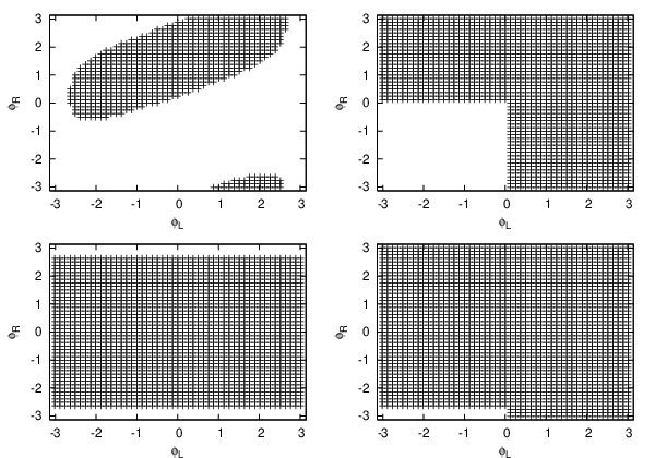
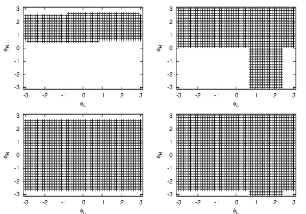
We would like to emphasize some advantages of our method for constraining the coupling. First of all, in obtaining our constraint no extra assumptions were made. In fact, although the result arises from a two-loop calculation, it is free of ultraviolet divergences and the expression given in Eq. (7) is exact since the parametric integral can be numerically evaluated for any external fermion, including even a very heavy one. Our result thus can be useful for predicting the EDM of the and leptons or the and quarks, for instance. In addition, our bound can be easily updated. Along these lines, in Ref. [14] a proposal was presented for improving the experimental limit of the EDM of the electron by orders of magnitude. This would lead to a bound on of the order of , which is of the same order of magnitude than that arising from meson physics. More recently, the nEDM Collaboration [15] has presented a proposal [16] to improve the current limit on the neutron EDM by orders of magnitude. This potential constraint would lower the bound on to the level of , which would be more stringent by about one order of magnitude than those obtained from meson physics and the CLEO data.
In closing we would like to emphasize the relevance of the present work. Important information on the origin of CP violation may be extracted from the measurement of the EDM of elementary particles. Several sources of CP violation are predicted in beyond-the-SM models, and the most stringent experimental limits imposed on the EDM of the electron or the neutron would allow us to asses their relative importance or eventually to rule them out. In this paper, we have studied the impact of a complex phase associated with the most general renormalizable coupling with both left- and right-handed components on the EDM of an arbitrary fermion. For the sake of completeness, the calculation of the two-loop amplitude was analyzed to some extent. The resultant expression can be straightforwardly used to predict the sensitivity of the EDM of a light or heavy fermion to a complex phase appearing in the coupling. In particular, our theoretical result was numerically evaluated in the scenario of a light fermion and the outcome was combined with the experimental limits on the EDM of light fermions to obtain an inequality that can be easily updated to constrain the coupling. Using the most recent experimental constraints on the EDM of the electron and the neutron, it was found that the latter gives the most stringent bound on the complex phase, which is one order of magnitude less stringent than those obtained from meson physics. We would like to emphasize however that our bound could be improved by about two orders of magnitude if the neutron EDM is measured with more precision at a near future, as recently proposed [15].
Acknowledgments. We acknowledge financial support from CONACYT and VIEP-BUAP (México).
Appendix A The two loop calculation
Using the SM Feynman rules and the one induced by the Lagrangian (1), the amplitude for the coupling can be written as:
| (20) |
where is the two-loop vertex function, which is given by
| (21) | |||||
with the electric charge of the quark in units of the positron charge, the mass of the internal fermion that couples to the boson and the fermion, and
| (22) | |||||
| (23) |
| (24) | |||||
| (25) |
| (26) | |||||
| (27) | |||||
This amplitude generates contributions to all the form factors associated with the on-shell vertex, but we are only interested in the term proportional to . The latter can be isolated after the identity is used. After some algebra, the contribution to the EDM of can be written as
| (28) |
where is the sine of the weak angle. Note that the integrals in dimensions were written in four dimensions as they are free of ultraviolet divergences.
We will proceed to solve the two-loop amplitude. Using Feynman parameters for the integral over , one obtains
| (29) | |||||
where
| (30) | |||||
| (31) |
with and
| (32) | |||||
| (33) | |||||
| (34) |
Once the integral over is done, Feynman parametrization for the integral over leads to
| (35) | |||||
where we have introduced the following notation: , , and
| (36) |
The EDM of can thus be written as
| (37) |
where we have introduced the dimensionless variables and
| (38) |
with
| (39) | |||||
| (40) | |||||
| (41) | |||||
| (42) | |||||
| (43) | |||||
We can further simplify the parametric integral . Explicit integration over leads to
| (44) |
where
| (45) | |||||
It is not possible to solve the integrals over nor analytically, so numerical evaluation would be necessary. However, a relatively simple expression can be obtained in the limit, which is a good approximation for the case of a light fermion doublet coupling to the boson. This is suited for the purpose of our work as we will use the experimental limits on the EDM of the electron and the neutron to constrain the coupling. In such an approximation, once the integral over and are done, the parametric integral reduces to
| (46) |
where
| (47) | |||||
with . The second term between the square brackets can be integrated straightforwardly, whereas the term with the logarithm cannot be integrated in terms of elementary functions. The final result is given in Eq. (3).
References
- [1] J. H. Christenson, J. W. Cronin, V. L. Fitch, and R. Turlay, Phys. Rev. Lett. 13, 138 (1964); J. Alexander et al. [Heavy Flavor Averaging Group (HFAG) Collaboration], hep-ex/0412073; A. Soni, hep-ph/0509180.
- [2] For a recent review, see M. Pospelov and A. Ritz, Annals. Phys. 318, 119 (2005).
- [3] M. E. Pospelov and I. B. Khriplovich, Sov. J. Nucl. Phys. 53, 638 (1991)[Yad. Fiz.53, 1030 (1991)]; E. P. Shabalin, Sov. J. Nucl. Phys. 28, 75 (1978)[Yad. Fiz. 28, 151 (1978)]; F. Hoogeveen, Nucl. Phys. B341, 322 (1990); D. Chang, W. Y. Keung, and J. Liu, Nucl. Phys. B355, 295 (1991).
- [4] R. Arnowitt, M. J. Duff, and K. S. Stelle, Phys. Rev. D43, 3085 (1991); Pran Nath, Phys. Rev. Lett. 66, 2565 (1991); Y. Kizukuri and N. Oshimo, Phys. Rev. D45, 1806 (1992); idem. 46, 3025 (1992); C. Hamzaoui, M. Pospelov, and R. Roiban, Phys. Rev. D56, 4295 (1997); T. Kadoyoshi and N. Oshimo, Phys. Rev. D55, 1481 (1997); T. Ibrahim and P. Nath, Phys. Rev. D57, 478 (1998); A. Bartl, T. Gadjdosik, W. Porod, P. Stockinger, and H. Stremnitzer, Phys. Rev. D60, 073003 (1999); A. Pilaftsis, Phys. Lett. B471, 174 (1999); L. Clavelli, T. Gajdosik, and W. Majerotto, Phys. Lett. B494, 287 (2000); D. Chang, W-F. Chang, and W-Y. Keung, Phys. Lett. B478, 239 (2000); C-S. Huang and L. Wei, Phys. Rev. D62, 016008 (2000); D. Chang, W-F. Chang, Mariana Frank, and W-Y. Keung, Phys. Rev. D62, 095002 (2000); K. Choi, E. J. Chun, and K. Hwang, Phys. Rev. D63, 013002 (2000); Y-Y. Keum and O. C. W. Kong, Phys. Rev. Lett. 86, 393 (2001); V. Barger, T. Falk, T. Han, J. Jiang, T. Li, and T. Plehn, Phys. Rev. D64, 056007 (2001); D. Chang, W-F. Chang, and W-Y. Keung, Phys. Rev. D66, 116008 (2002); U. Chattopadhyay, T. Ibrahim, and D. P. Roy, Phys. Rev. D64, 013004 (2001); T-F. Feng, X-Q. Li, J. Maalampi, and X. Zhang, Phys. Rev. D71, 056005 (2005); D. Chang, W-F. Chang, W-Y. Keung, Phys. Rev. D71, 076006 (2005); T-F. Feng, X-Q. Li, J. Maalampi, H-S. Song, Phys. Rev. D73, 116001 (2006); D. A. Demir and Y. Farzan, arXiv:hep-ph/0610181 (2006); S. Y. Ayazi and Y. Farzan, arXiv:hep-ph/0702149 (2007).
- [5] G. Beall and M. G. Deshpande, Phys. Lett. B132, 427 (1983); S. Weinberg, Phys. Rev. Lett. 63, 2333 (1989); G. Valencia, Phys. Rev. D41, 1562 (1990); S. M. Barr and A. Zee, Phys. Rev. Lett. 65, 21 (1990); J. F. Gunion and R. Vega, Phys. Lett. B251, 157 (1990); R. G. Leigh, S. Paban, and R-M. Xu, Nucl. Phys. B352, 45 (1991); D. Chang, W-Y. Keung, and T. C. Yuan, Phys. Rev. D43, R14 (1991); C. Kao and R-M. Xu, Phys. Lett. B296, 435 (1992); D. Bowser-Chao, D. Chang, and W-Y. Keung, Phys. Rev. Lett. 79, 1988 (1997).
- [6] G. Beall and A. Soni, Phys. Rev. Lett. 47, 552 (1981); G. Ecker, W. Grimus, and H. Neufeld, Nucl. Phys. B229, 421 (1983); J. F. Nieves, D. Chang, and P. B. Pal, Phys. Rev. D33, 3324 (1986); D. Chang, C. S. Li, and T.C. Yuan, Phys. Rev. D42, 867 (1990); F. Atwood, C. P. Burgess, C. Hamzaoui, B. Irwin, and J. A. Robinson, Phys. Lett. B256, 471 (1991); J.-M. Frere, J. Galand, A. Le Yaouanc, L. Pliver, O. Pene, and J.-C. Raynal, Phys. Rev. D45, 259 (1992); D. Chang, A.-G. He, W.-Y. Keung, B. H. J. McKellar, and D. Wyler, Phys. Rev. D46, 3876 (1992); M. Frank, Phys. Rev. D59, 055006 (1999); M.-C. Chen and K. T. Mahanthappa, Phys. Rev. D75, 015001 (2007).
- [7] S. M. Barr and A. Masiero, Phys. Rev. Lett. 58, 187 (1987); A. De Rújula, M. B. Gavela, and F. J. Vegas, Phys. Lett. B245, 640 (1990); J. F. Gunion and D. Wyler, Phys. Lett. B248, 170 (1990); A. S. Joshipura, Phys. Rev. D43, R25 (1991); D. Chang, K. Choi, and W.-Y. Keung, Phys. Rev. D44, 2196 (1991); M. J. Ramsey-Musolf, Phys. Rev. Lett. 83, 3997 (1999); Y. Liao and X. Li, Phys. Rev. D61, 076002 (2000); M. Pospelov and A. Ritz, Phys. Rev. D63, 073015 (2001); J. P. Archambault, A. Czarnecki, and M. Pospelov, Phys. Rev. D70, 073006 (2004); C. Dib, A. Faessler, t. Gutschet, S. Kovalenko, J. Kuchei, V. Lyubovitskij, and K. Pumsa-ard, J. Phys. G32, 547 (2006).
- [8] W.-M. Yao et al., J. Phys. G33, 1 (2006).
- [9] C. A. Baker et al., Phys. Rev. Lett. 97, 131801 (2006) [arXiv:hep-ex/0602020].
- [10] M. Pospelov, Phys. Lett. B 530, 123 (2002) [arXiv:hep-ph/0109044].
- [11] A. Abd El-Hady and G. Valencia, Phys. Lett. B414, 173 (1997).
- [12] F. Larios, M. A. Pérez, and C. P. Yuan, Phys. Lett. B457, 334 (1999).
- [13] K. Fujikawa and A. Yamada, Phys. Rev. D 49, 5890 (1994).
- [14] M. G. Kozlov, and A. Derevianko, Phys. Rev. Lett. 97, 063001 (2006).
- [15] The nEDM Experiment (M. D. Cooper and S. K. Lamoreaux spokespersons) http://p25ext.lanl.gov/edm/edm.html.
- [16] T. M. Ito, arXiv:nucl-ex/0702024 (2007).