Dark-State Polaritons in Single- and Double-$\Lambda$ Media

Several years ago, Fleischhauer and Lukin Lukin predicted the existence of a stable polaritonic excitation in $\Lambda$-type media [Fig. 1(a)] exhibiting electromagnetically-induced transparency (EIT) EIT. This excitation, which involves a vanishing population of excited states and was therefore dubbed the “dark-state polariton” (DSP), is a coherent quantum excitation whose evolution is governed by a classical control field. This provides a method for manipulating single-photon motion, including stopping light Phillips; Hau. The Fleischhauer-Lukin result was derived as a perturbation expansion of the field operator equations of motion in the strong control field limit. In a subsequent work, Juzeliūnas and Carmichael used a Bogoliubov-type transformation to diagonalize the model Hamiltonian exactly, and showed that the DSP can be understood as a part of a branch of slow polaritons occurring in systems containing a pair of atomic resonances Juz. These authors also emphasized the fact that the photonic part of the polariton mixes with atomic excitations possessing wavevectors differing by the wavevector of the control field. Thus, for instance, it is possible to reverse the direction of a polariton wavepacket by switching the direction of the control field.

In this paper, we derive the properties of the DSP using the Sawada-Brout technique SB. This can be thought of as a simplified version of the method used by Juzeliūnas and Carmichael, and we shall see how its results reduce to those of Fleischhauer and Lukin near resonance, which was not demonstrated in Ref. Juz. We then extend the analysis to a double-$\Lambda$ medium [Fig. 1(b)], which contains a DSP consisting of low-lying atomic excitations and photon states of two different frequencies Raczynski; Li. In both single- and double-$\Lambda$ systems, the DSP is protected against incoherent decay processes acting on the excited states, because it contains a vanishing population of these states. It has previously been shown that double-$\Lambda$ media can efficiently upconvert classical probe beams Korsunsky; Merriam, and a related four-wave mixing scheme has already been used in such systems to generate correlated photon pairs Kolchin; Braje; Balic; Thompson. Here, we point out that the DSP could be exploited to perform single-photon frequency conversion in a manner that preserves quantum coherence. Unlike semiclassical analyses in which the electromagnetic field is treated classically Korsunsky; Merriam, this theory applies to the single-photon regime. It may thus have applications in quantum information processing, such as for downconverting a member of an entangled photon pair to a frequency suitable for transmission over a telecommunications fiber. Unlike parametric conversion schemes exploiting optical nonlinearities, the relevant photons are up- or down-converted individually, instead of being split or recombined; the additional momentum and energy are supplied by the control fields.

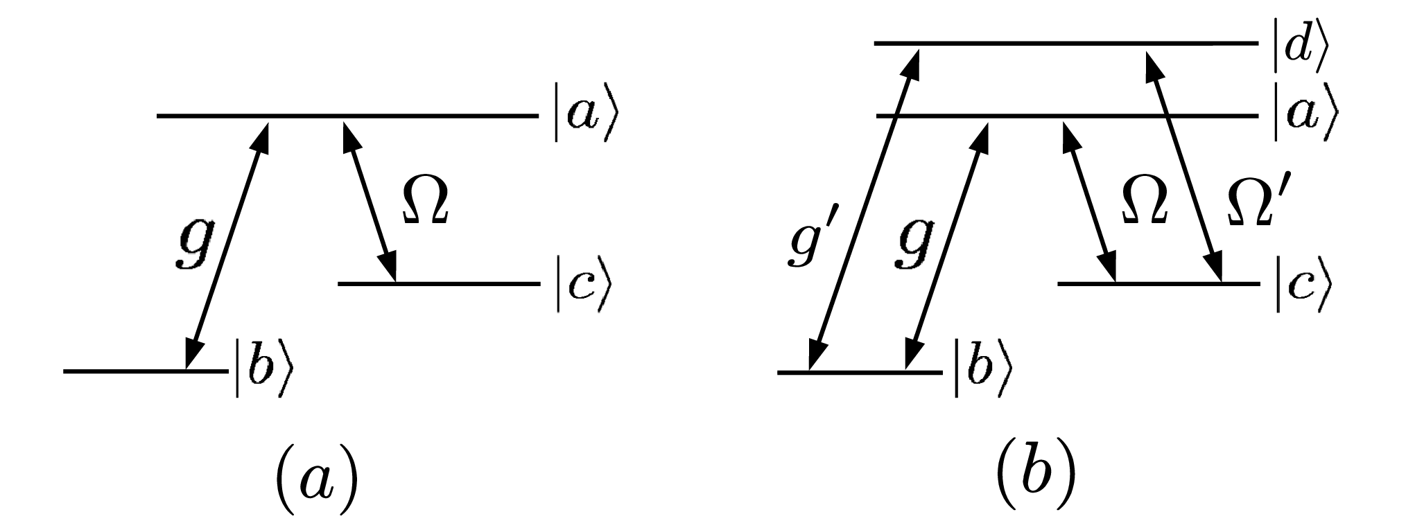
We begin by considering an $N$-atom gas with a single-$\Lambda$ level structure, shown in Fig. 1(a). The ground, excited, and metastable atomic states are respectively denoted by $\left|b\right\rangle$, $\left|a\right\rangle$, and $\left|c\right\rangle$, and their corresponding energies by $\hbar\omega_{b}$, $\hbar\omega_{a}$, and $\hbar\omega_{c}$. The atomic Hamiltonian is

with the sum performed over all atomic positions $r$. Here,

denotes a transition operator for the atom at position $r$. We also define Fourier-transformed operators, $\sigma^{ab}_{k}\equiv N^{-1/2}\sum_{r}\sigma^{ab}_{r}\,e^{ikr}$ etc. The photon Hamiltonian is

where $a_{k}^{\dagger}$ and $a_{k}$ are photon creation and destruction operators. The photons interact with the $ab$ transition through the minimal-coupling Hamiltonian

The coupling constant is $g\simeq\mathcal{P}\sqrt{2\pi N\omega_{ab}/\hbar V}$, where $\mathcal{P}$ is the dipole moment of the $ab$ transition, $\omega_{ab}\equiv\omega_{a}-\omega_{b}$, and $V$ is the cavity volume. For notational simplicity, we have used the rotating-wave approximation. Finally, we include a classical control field with strength (Rabi frequency) $\Omega$, frequency $\omega_{L}\sim\omega_{ac}$, and wavevector $k_{L}$:

Here, we have again discarded counter-rotating terms. We neglect the coupling between the photons and the $ac$ transition, which is negligible compared to the effects of the control field, and the coupling between the control field and the $ab$ transition, which is off resonance.

The time dependence in (5) can be removed by defining

where $H(t)\equiv H_{0}+\cdots+H_{3}(t)$, and

The Schrödinger equation $H(t)\left|\psi(t)\right\rangle=i\hbar\partial_{t}\left|\psi\right\rangle$ can be then rewritten as

Thus, we can extract solutions to the Schrödinger equation from the energy eigenstates of the time-independent Hamiltonian $H_{L}$. To obtain these, we look for a polariton excitation operator $A^{\dagger}$ such that

The polariton is long-lived provided the omitted terms are negligible SB. If the initial state of the system is its (zero photon) ground state, $A^{\dagger}$ should be a mixture of $a^{\dagger}$, $\sigma^{ab}$, and $\sigma^{cb}$. Below, we list the commutation relations of these three operators with $H_{L}$. We have removed terms involving $\sigma^{ba}$, $\sigma^{aa}$, $\sigma^{ca}$, and $a_{k}$; since these operators give zero when acting on the ground state, this introduces no additional error for single-polariton excitations. Similarly, we have replaced $\sigma^{bb}_{k}$ with $\sqrt{N}\delta_{k0}$. Thus,

Let us now look for excitation operators of the form

where the band index $n$ enumerates the different polariton species. The c-numbers $\phi^{j}_{nk}$ are determined by inserting (13) into (9) and using (10)-(12). This gives three self-consistency equations that can be written as

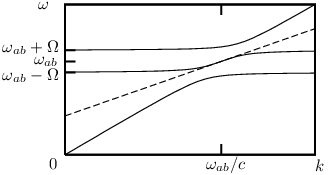
The form of the effective Hamiltonian in (14) is familiar from semiclassical analyses of EIT. Fig. 2 shows the bandstructure in the absence of loss, similar to the one given in Ref. Juz. For simplicity, let us assume that $\omega_{L}=\omega_{ac}$. The asymptotic eigenfrequencies far from resonance are $c|k|$ and the eigenvalues of the upper-left $2\times 2$ submatrix in the effective Hamiltonian, in this case $\omega_{ab}\pm\Omega$. Exactly at resonance ($|k|=\omega_{ab}/c$), there is an eigenvector $\propto[0,1,-\Omega/g]$, and for slightly detuned $k$ this eigenvector continues into ones where the $\sigma^{ab}$ component is nonzero but small. These solutions—“dark-state polaritons”—are thus insensitive to incoherent decay processes acting on $\left|a\right\rangle$. The stability of the exactly-resonant DSP is limited only by the lifetime of the metastable state $\left|c\right\rangle$, which we shall assume to be longer than the time-scale of any relevant experiment. For off-resonant DSPs, the decay rate is only quadratic in the detuning: upon replacing $\omega_{a}$ with $\omega_{a}-i\Gamma_{a}$ in (14), one finds that the imaginary part acquired by $\omega_{k}$ is $\sim\Gamma_{a}|\Delta/\Omega|^{2}$ (for $\Omega\gg g$), where $\Delta\equiv c|k|-\omega_{ab}$. The other two polariton branches correspond to “bright” polaritons that contain significant $\left|a\right\rangle$ population and are thus strongly affected by losses. As in Ref. Lukin, we neglect Langevin noise effects, which do not influence the adiabatic evolution of the DSPs.

Expanding around $\omega=\omega_{ab}$ yields a limiting solution for the DSPs:

Eq. (15-17) agree with the solution derived by Fleischhauer and Lukin using a perturbation expansion in $1/\Omega$ Lukin. In our formalism, the fact that decreasing $\Omega$ reduces the polaritonic group velocity can be intuitively understood as the result of “squeezing” the bandwidth of the middle polariton band. An interesting property of the DSP solution is that it does not depend on the energies of the underlying $\Lambda$ system, only the detuning of the control field and the coupling parameters $g$ and $\Omega$.

Finally, we can extract the solutions to the original Schrödinger equation using (8). For a polariton with quantum numbers $(n,k)$, the state at time $t$ is

The $\sigma^{cb}$ component in (18) has a different frequency and wavevector compared to the rest of the polariton. This property does not, however, destabilize the polariton: in a wavepacket constructed of a superposition of DSPs, the photonic and $\sigma^{cb}$ components possess different phase factors but share a single envelope.

The preceding derivation holds regardless of the angle between the input photon and the control beam. The direction of $k_{L}$ only enters into the choice of excitation operator $\sigma_{k-k_{L}}^{cb}$ occurring in the polariton operator (13), and plays no role in the eigenproblem (14) that yields the state amplitudes and polariton energy.

By switching between two non-collinear control beams, it is possible to coherently rotate the photon wavevector, by an angle of up to $2\sin^{-1}(\omega_{ac}/\omega_{ab})$, where the plane of rotation is specified by the polarization of the control field. A special case of this has been discussed by Juzeliūnas and Carmichael: when $\omega_{b}\approx\omega_{c}$, one can coherently backscatter the photon by inserting a photon with $k\sim k_{L}$, which mixes with a $\sigma^{bc}$ excitation with wavevector $k-k_{L}\sim 0$, and switching the control field to $-k_{L}$. The $\sigma^{bc}$ excitation then mixes into a photon of wavevector $k-2k_{L}\sim-k$ Juz.

Suppose we add a second excited state, $\left|d\right\rangle$, as shown in Fig. 1(b). A second control beam couples $\left|d\right\rangle$ to $\left|c\right\rangle$, and for simplicity we assume that the two control beams have parallel polarization vectors. The $d\leftrightarrow a$ transition is assumed to be forbidden. One of the reasons this “double-$\Lambda$” system is interesting is that it can be used to upconvert or downconvert probe beams, as experimentally demonstrated by Merriam et. al. Merriam and other groups. It can be shown, using the Fleischhauer-Lukin formalism, that this type of level structure supports a DSP Li. As we shall see, this DSP arises naturally from the present method as a $5\!\times\!5$ generalizion of (14).

The Hamiltonian, $H^{\prime}(t)$, contains four new terms. The first, $\sum_{r}\omega_{d}\sigma^{dd}_{r}$, gives the energy of the $\left|d\right\rangle$ states. Next, we introduce a second photon field with operators $b_{k}^{\dagger}$ and $b_{k}$, and Hamiltonian $\sum_{k}\hbar c|k|b_{k}^{\dagger}b_{k}$. (There is really only one photon field, but this trick is permissible since the atom-photon coupling becomes negligible far away from the EIT resonances.) Finally, we add interaction terms analogous to (4) and (5), with $\left|d\right\rangle$, $b_{k}$, $g^{\prime}$, and $\Omega^{\prime}$ replacing $\left|a\right\rangle$, $a_{k}$, $g$, and $\Omega$ respectively.

The control field interaction Hamiltonian (5) and its analog for the $dc$ transition oscillate at different frequencies, so the transformation (6)-(7), which works by rotating $\left|c\right\rangle$, cannot eliminate the time dependence. We can overcome this difficulty with a transformation that instead rotates the $\left|a\right\rangle$, $\left|d\right\rangle$, and photonic states. Let

where $H^{\prime}(t)$ is our new Hamiltonian, and

This once again allows us to write the Schrödinger equation as $i\hbar\partial_{t}\left[U_{L}^{\prime}(t)\left|\psi(t)\right\rangle\right]=H_{L}^{\prime}\left[U_{L}^{\prime}(t)\left|\psi(t)\right\rangle\right]$, where $H_{L}^{\prime}$ is time-independent. We look for excitation operators for $H_{L}^{\prime}$ of the form

The self-consistency equations for the parameters $\phi^{j}_{nk}$ take the same matrix form as (14), with effective Hamiltonian

The polariton created by (21) is a valid excitation because, as in the single-$\Lambda$ case, no extra non-negligible terms are generated by commutating this operator with the Hamiltonian. Let us now assume that the control fields are resonant, i.e. $\omega_{L}=\omega_{ac}$ and $\omega_{L}^{\prime}=\omega_{dc}$. For $|k+k_{L}|=\omega_{ab}/c$ and $|k+k_{L}^{\prime}|=\omega_{db}/c$, the effective Hamiltonian (22) has an eigenvector $\propto[0,0,1,-\Omega/g,-\Omega^{\prime}/g^{\prime}]$. The first two components of this eigenvector, corresponding to the two excited states, are identically zero, so this represents a DSP consisting of $\sigma^{cb}_{k}$ excitations and photons with wavevectors $k+k_{L}$ and $k+k_{L}^{\prime}$. It can be shown that no other linearly independent eigenvector with this property exists, so there is only one such DSP solution. The linearized DSP solution, analogous to (15)-(17), is

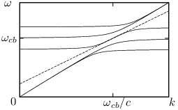
where $\delta k\equiv|k+k_{L}|-\omega_{ab}/c$ and $\delta k^{\prime}=|k+k_{L}^{\prime}|-\omega_{db}/c$. The polaritonic bandstructure, in the absence of loss, is shown in Fig. 3.

These results can be shown to be consistent with the single-photon limit of a semiclassical analysis of the double-$\Lambda$ medium given by Korsunsky and Kosachiov Korsunsky. In this one-dimensional model, where the electromagnetic field is treated classically, the Heisenberg equations of motion for the atomic system possesses a stationary “dark state” solution that is decoupled from the electromagnetic field and is stable against spontaneous emission. This dark state exists only if the background field (consisting of two probe beams and two control beams) obeys certain frequency, amplitude, and phase matching conditions. The frequency-matching condition is

where $\omega$ and $\omega^{\prime}$ are the respective frequencies of the probe beams resonant with the $ab$ and $db$ transitions. This equation is exactly satisfied by (21), for which $\omega=c(k+k_{L})$ and $\omega^{\prime}=c(k+k_{L}^{\prime})$. The physical meaning of (28) is particularly easy to deduce in the present theory: in the single-photon limit, the stationary state corresponds to a polaritonic solution of the form (21), for which the photonic components cannot take on arbitrary frequencies because they are coherently mixed via the atomic excitation $\sigma^{cb}_{k}$. The amplitude-matching condition for the semiclassical dark state is

where $\mathcal{P}$ and $\mathcal{P}^{\prime}$ are the dipole moments for the $ab$ and $db$ transitions, and $E$ and $E^{\prime}$ are the electric field amplitudes of the associated probe beams. The electric field amplitudes can be related to the quantum mechanical photon amplitudes $\phi^{4}$ and $\phi^{5}$ by

which can be verified by computing the expectation value $\langle|E|^{2}\rangle$ produced by each photon creation operator. With this identification, the linearized DSP amplitudes (26) and (27) satisfy (29). The third condition derived by Korsunsky and Kosachiov, which relates the phases of the four beams, is also satisfied by the DSP because, as shown by (26) and (27), the phases of the probe beams are locked to those of the control beams $\Omega$ and $\Omega^{\prime}$.

The dark state studied by Korsunsky and Kosachiov is a pure state of the atomic system, reflecting the fact that the electromagnetic field is treated classically Korsunsky. In contrast, the present model takes into account the coherent mixing between the quantum state of the probe field and the quantum state of the atomic medium: performing a partial trace of the DSP over the photonic Hilbert space yields a mixed atomic state. This mixing becomes important at the single-photon level, which is also potentially the regime of interest for quantum information processing. In the following section, we will examine how this mixing can be used to convert between the two photonic components of the double-$\Lambda$ DSP.

For a single-$\Lambda$ medium with a resonant control beam, inserting a photon with wavevector $k_{0}$, resonant with the $ab$ transition, gives rise to a DSP whose group velocity points in the same direction, independent of the direction of the control beam. This freedom to choose the direction of the control beam disappears in the double-$\Lambda$ case. Here, an incident photon $k_{0}$ mixes with another photon with wavevector $k_{1}=k_{0}-k_{L}+k_{L}^{\prime}$. Assuming both control beams are tuned to resonance, the resulting state overlaps with a DSP only if $|k_{1}|\simeq\omega_{db}/c$. Furthermore, the group velocity of the DSP is, from (23),

where $\hat{k}_{0}=k_{0}/|k_{0}|$ and $\hat{k}_{1}=k_{1}/|k_{1}|$. Therefore, a choice of $\hat{k}_{0}$ and $\hat{k}_{1}$ determines the directions of the two control beams (or, more generally, choosing any two of these directions determines the other two). As an aside, we note that the beam matching conditions forbid the choice $\hat{k}_{0}=-\hat{k}_{1}$, which would imply the possibility of a stationary wavepacket with nonzero control beams; however, if $\hat{k}_{0}$ and $\hat{k}_{1}$ are nearly antiparallel, (32) predicts that the control beam strengths can be tuned to produce a low group velocity.

In order to illustrate the mixing between the two photonic components in the DSP, let us fall back on the “trivial” one-dimensional case where all wavevectors are parallel, which satisfies the above beam matching conditions. Suppose we inject the photon $k_{0}$ at $t=0$, so that the quantum state is

where $k\equiv k_{0}-k_{L}$. Without losses, the state at time $t$ is

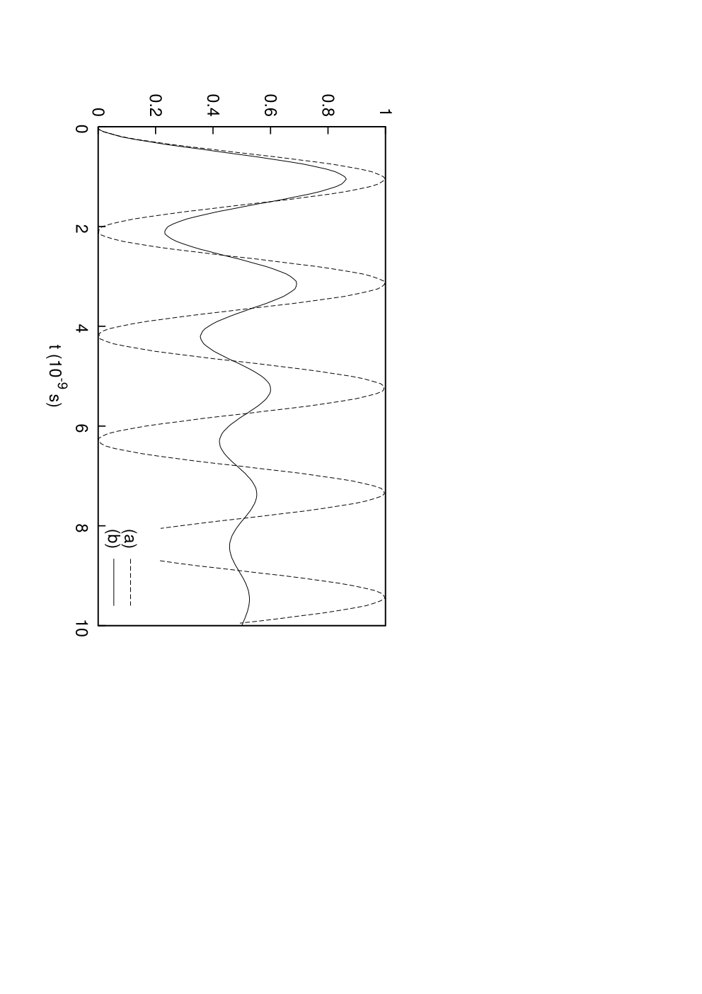
where the matrix $\mathcal{H}$ is defined in (22) and the omitted terms are the other polariton components. The result, shown in Fig. 4, is an oscillating upconversion amplitude $|\left\langle 0\right|b_{k+k_{L}^{\prime}}\left|\psi(t)\right\rangle|$ that can approach 100%. The effects of incoherent excited state decay, which can be modeled by replacing $\omega_{a}$ with $\omega_{a}-i\Gamma_{a}$ and $\omega_{d}$ with $\omega_{a}-i\Gamma_{d}$ in (22), are also shown in Fig. 4. Although the DSPs are protected against decay, damping still occurs because the incident photon generates a non-vanishing population of bright polaritons. When these exit the system (typically as off-axis photons), only the DSP remains.

A more efficient example of single-photon frequency conversion can be obtained by going from momentum space to real space and studying the behavior of polariton wavepackets. Let us define c-number fields $\Phi_{j}=\Phi_{j}(r,t)$ such that

Inserting (35) into the Schrödinger equation and using (22), we obtain a Schrödinger wave equation

If $\kappa$ is chosen such that $|\kappa+k_{L}|=\omega_{ab}/c$ and $|\kappa+k_{L}^{\prime}|=\omega_{db}/c$, then the DSP corresponds to values of $\Phi_{j}$ that are constant in space. For a wavepacket centered around $\kappa$ with bandwidth $\ll\omega_{ab},\,\omega_{db}$ (i.e., spatial width much longer than the optical wavelength, which is the usual slowly-varying envelope approximation), $\mathcal{H}$ takes on the intuitive local form

As in the single-$\Lambda$ case, the evolution of the polaritonic envelope is independent of the underlying double-$\Lambda$ frequencies, except through the coupling parameters $g$, $g^{\prime}$, $\Omega$, and $\Omega^{\prime}$. We again emphasize that this result is not perturbative; it holds for arbitrary values of $\Omega$ and $\Omega^{\prime}$, and depends only on the fact that the wavepacket is sufficiently broad. Generally, the coupling parameters can vary (smoothly) in space; for instance, a variation in $\Omega$ or $\Omega^{\prime}$ could be accomplished using a c.w. control beam with a non-uniform cross-sectional intensity profile. Such variations can be used to “adiabatically” transfer one photon population to another within a propagating DSP wavepacket, substantially improving the efficiency of the conversion process compared to the previous example.

Let us consider an effectively one-dimensional experimental setup where all relevant spatial variations occur in the $z$ direction. In particular, we must assume that the $x$ and $y$ edges are far enough away that boundary effects (which appear when the beams are not all collinear) are negligible. The incident envelope field $\Phi_{j}(z,t=0)$ is

Outside the sample ($z<0$ or $z>z_{0}$), all coupling parameters are zero. Within the sample ($0<z<z_{0}$), the functional forms of $\Omega(z)$ and $\Omega^{\prime}(z)$ are chosen so that $|\Omega|\gtrsim|g|\gtrsim|\Omega^{\prime}|$ near the entrance of the sample, which ensures that the DSP is dominated by the input photon; whereas $|\Omega^{\prime}|\gtrsim|\Omega|\gtrsim|g|$ near the exit, which ensures that the DSP is dominated by the converted photon. The result is shown in Fig. 5. For the given parameters, the converted photon amplitude is $\sim 0.9$ times the incident amplitude. The efficiency is limited by the available length of the double-$\Lambda$ medium. As shown in Fig. 6, a longer sample allows the $\Omega^{\prime}$ field to be varied more gently, generating fewer bright state polaritons and increasing the conversion efficiency.

In this paper, we have presented an analysis of single- and double-$\Lambda$ EIT systems based on a microscopic equation-of-motion technique. Within this formalism, the presence of a DSP corresponds to the existence of special eigenvectors of an effective Hamiltonian matrix, in which the entries corresponding to rapidly decaying excitations are identically zero, regardless of the strength of the control fields. The ability of the double-$\Lambda$ system to efficiently upconvert and downconvert photons, previously established in semiclassical four-wave mixing studies Korsunsky; Merriam, is retained in the coherent single-photon limit due to the existence of the DSP. The analysis can be further generalized to multi-$\Lambda$ systems, where one finds additional polaritonic bands similar to those in Fig. 3, with exactly one family of DSP solutions possessing vanishing excited state populations.

Throughout this paper, we have restricted our attentions to the single-polariton sector of the theory, which is valid only if the polaritons are much more dilute than the underlying atomic medium. The polariton operators (13) and (33) do not obey exact bosonic commutation relations, since the $\sigma$ operators are not bosonic operators; however, the corrections to the commutator vanish as $O(M/N)$, where $M$ is the number of atoms excited Hopfield. This condition is satisfied, for instance, in the experiments of Merriam et. al., where $M/N\sim 10^{-3}$ Merriam. The single-polariton sector has the advantage that the quantum state of the system can be expressed in terms of a simple wave equation, as in (36). Thus, once the $\sigma$ operators have been used to derive the effective Hamiltonian, the additional structure given by their non-trivial commuation relations disappears from the theory. Should one wish to study the limit where $M$ becomes comparable to $N$, this structure will have to be taken into account.

We would like to thank P. Bermel, S. E. Harris, J. Taylor, and V. Vuletic for helpful comments. This work was supported in part by the Army Research Office through the Institute for Soldier Nanotechnologies under Contract No. W911NG-07-D-0004, and by DOE Grant No. DE-FG02-99ER45778.

References

- (1) M. Fleischhauer and M. D. Lukin, Phys. Rev. Lett. 84, 5094 (2000); Phys. Rev. A 65, 022314 (2002).
- (2) S. E. Harris, Phys. Today 50 (7), p.36 (1997).
- (3) D. F. Phillips, A. Fleischhauer, A. Mair, R. L. Walsworth, and M. D. Lukin, Phys. Rev. Lett. 86, 783 (2001).
- (4) C. Liu, Z. Dutton, C. H. Behroozi, and L. V. Hau, Nature 409, 490 (2001).
- (5) G. Juzeliūnas and H. J. Carmichael, Phys. Rev. A 65, 021601(R) (2002).
- (6) K. Sawada, Phys. Rev. 106, 372 (1957); R. Brout, Phys. Rev. 108, 515 (1957).
- (7) A. Raczyński, J. Zaremba, and S. Zielśka-Kaniasty, Phys. Rev. A 69, 043801 (2004).
- (8) Z. Li, L. Xu, and K. Wang, Phys. Lett. A 346, 269 (2005).
- (9) E. A. Korsunsky and D. V. Kosachiov, Phys. Rev. A 60, 4996 (1999).
- (10) A. J. Merriam, S. J. Sharpe, M. Shverdin, D. Manuszak, G. Y. Yin, and S. E. Harris, Phys. Rev. Lett. 84, 5308 (2000).
- (11) P. Kolchin, Phys. Rev. A 75, 033814 (2007).
- (12) D. A. Braje, V. Balic, S. Goda, G. Y. Yin, and S. E. Harris, Phys. Rev. Lett. 93, 183601 (2004).
- (13) V. Balic, D. A. Braje, P. Kolchin, G. Y. Yin, and S. E. Harris, Phys. Rev. Lett. 94, 183601 (2005).
- (14) J. K. Thompson, J. Simon, H. Loh, and V. Vuletic, Science 313, 74 (2006).
- (15) J. J. Hopfield, Phys. Rev. 112, 1555 (1958).