Cosmic rays from thermal sources

For relativistic particles (where the rest mass $m$ can be neglected) the energy $E\sim p$ and the density of states of an ideal gas in three dimensions is given by $\omega(E)\propto E^{2}$. The flux $\Phi(E)$ can be then obtained straightforwardly from $P(E)$ and reads

where $N_{0}$ is normalization factor. For $E>>T$ we have power spectrum $\Phi(E)\propto E^{-\gamma}$ with the slope parameter $\gamma$ which in terms of parameter $q$ introduced above is $\gamma=(3-2q)/(q-1)$. In the case of CR this spectrum has the shape of broken power law $E^{-\gamma}$ which changes pattern in the region named as ”knee” with the slope $\gamma_{1}\simeq 2.7$ at energies below $\sim 10^{15}$ eV and $\gamma_{2}\simeq 3.1$ at energies between the ”knee” and the highest measurable energies $E\sim 10^{18}$ eV. In the language of the nonextensivity parameters it would mean that $q_{1}=1.213$ before and $q_{2}=1.196$ after the ”knee”, i.e., one can argue then that at the ”knee” one witnesses the change of fluctuation pattern.

As mentioned above the special role in converting exponential distribution to its $q$-exponential counterpart play fluctuations of the scale parameter provided in the form of gamma function. There are at least two scenarios leading to gamma distribution in $\beta$ mentioned above (here $\mu^{-1}=\beta_{0}(q-1)$ and $\nu^{-1}=q-1$):

• $(a)$

  temperature distribution of sources;

• $(b)$

  temperature fluctuations in small parts of a source.

In what concerns the first possibility notice that gamma distribution (9) is the most probable outcome of the maximalization of Shannon information entropy (1) under constraints that $\int f(\beta)d\beta=1$, $\langle\beta\rangle=\beta_{0}$ and (because distribution we are looking for is one sided, i.e., defined only for $\beta>0$) that $\langle\ln(\beta)\rangle=\ln\left(\nu\beta_{0}\right)$. However, this possibility is rather unlikely because in this case one expects that there is some cut temperature $T_{cut}$ such that $T<T_{cut}$, which would result in very characteristic rapid break in the CR energy spectrum, not observed in experiment.

To illustrate the second possibility let us suppose that one has thermodynamic system, different small parts of which have locally different temperatures, i.e., its temperature understand in the usual way fluctuates. Let $\xi(t)$ describes the stochastic changes of temperature in time and let it be defined by the white Gaussian noise ($\langle\xi(t)\rangle=0$ and $\langle\xi(t)\xi(t+\Delta t)\rangle=2D\delta(\Delta t)$). The inevitable exchange of heat which takes place between the selected regions of our system leads ultimately to the equilibration of temperature. As we have advocated in [5], the corresponding process of the heat conductance leads eventually to the gamma distribution $f(\beta)$ (9) with variance (7) related to the specific heat capacity $C_{V}$ of the material composing this system by

The change of fluctuation pattern in the ”knee” region mentioned before would therefore correspond in this case to abrupt change in the heat capacity of the order of $C_{2}/C_{1}=1.09$.

Can one expect something of this kind to happen in the astrophysical environment of the CR? In what follows we shall argue that, indeed, one can. Let us first notice that subject of temperature fluctuations in astrophysics is much-discussed problem nowadays. Its effect on the temperatures empirically derived from the spectroscopic observation was first investigated in [7] whereas in [8, 9, 10, 11] it was shown that temperature fluctuations in photoionized nebulea have great importance to all abundance determinations in such objects. It means that discussion of the heat capacity or, equivalently, the behavior of parameter $q$ defining the energy spectrum, is fully justified.

Let us concentrate therefore on the problem of heat capacity of astrophysical objects, in particular in neutron stars. In such objects one observes the following feature. The total specific heat of their crust, $C$, is the sum of contributions from the relativistic degenerate electrons, from the ions and from degenerate neutrons. In the temperature that can be reached in the crust of an acreating neutron star (which is of the order of $T\sim 5\cdot 10^{8}$ K and is below the Debaye temperature $T_{D}\sim 5\cdot 10^{9}$ K) we have $C_{ion}<C_{e}<C_{n}$. When the temperature drops below the critical value $T=T_{C}$ the neutrons become superfluid and their heat capacity $C^{sf}_{n}$ increases [12, 13],

At $T\sim 0.7T_{C}$ we have $C^{sf}_{n}\sim 1.1C_{n}$ what corresponds to the changes of spectral index by $\Delta\gamma\sim 0.5$. To summarize: one witnesses here the abrupt change in the heat capacity at some temperature.

Suppose now that we take seriously the conjecture expressed by eq. (10) that $C_{V}$ is directly connected with the parameter $q$. It means then that, the usual fluctuation pattern given by gamma distribution (9) should be replaced by it slightly modified version shown in Fig. 1, which is characterized by two nonextensivity parameters, $q_{1}$ and $q_{2}$. This change is assumed to be abrupt and taking place at some temperature $T_{cut}$ and it differs our proposition from what was proposed in [2], which from our point of view, corresponds to some form of composition of two (suitably normalized) such gamma functions with different $q$ each. Following our proposition one obtains the following flux of CR:

where $P_{q}(E)$ is given by eq. (5) and

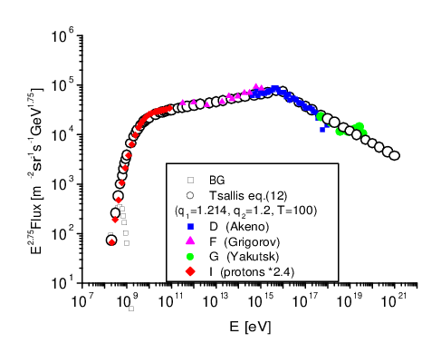
Our results are presented in Fig. 2. The ”knee” region is reproduced very well, however, the price to be paid is the need of suitable choice of energy at which fluctuation pattern changes (cf. Fig. 1)¹¹ 1 Two remarks are in order at this point. First, the nucleon superfluidity was predicted already in [14] and today pulsar glitches provide strong observational support for this hypothesis [15]. Nucleon superfluidity arises from the formation of Cooper pairs od fermions (actually in [16] also quark superfluidity from cooling neutron stars were investigated). Continuous formation and breaking of the Cooper pairs takes place slightly below $T=T_{C}$ (critical temperature $T_{C}$ is in the order $10^{9}-10^{10}$ K). The other, neutron stars are born extremely hot in supernova explosions, with interior temperatures around $T\sim 10^{12}$ K. Already within a day, the temperature in the cental region of the neutron star will drop down to $\propto 10^{9}-10^{10}$ K and will reach $10^{7}$ K in about $100$ years [17]. The first measurements of the temperature of a neutron star interior (core temperature of the Vela pulsar is $T\sim 10^{8}$ K, while the core temperature of PSR B0659+14 and Geminga exceeds $2\cdot 10^{8}$ K) allow to determine the critical temperature $T_{C}\sim 7.5\cdot 10^{9}$ K [18]..

As one can see in Fig. 2 we have obtained agreement with data for the whole range of CR energy spectrum but the price paid for this is, again, apparently too high value of the temperature parameter used, $T=100$ MeV. We have prone therefore to the same kind of criticism as we have applied to previous attempts in this field [2, 3]. The possible way out of this dilemma is to argue that the break in the original spectrum and connected with it phase transition occurs actually at much slower energies and that resultant spectrum is then accelerated to the observed energies - for example by the magneto-hydrodynamical turbulence and/or shock discontinuities (i.e., by the so called DSA mechanism, cf. [19]). The simplest version of this mechanism, as discussed in [20], implies that distribution function after the shock, $f_{after}(p)$, is related to the original distribution before the shock, $f_{before}(p)$ in the following way:

where $b=3r/(r-1)$. Here $p$ denotes the particle momentum, $r=\rho_{2}/\rho_{1}$ describes the compression of densities across the shock and $p_{min}$ denotes the minimal value of momenta. DSA mechanism transforms a $\delta\left(p-p_{0}\right)$ spectrum of relativistic particles in a power-like spectrum of the type $f(p)\propto p^{-b}$. For example, if one has initial spectrum of the form $\propto p^{-c}$ which encounters a shock with strength given by $b$ then eq. (13) shows that:

• •

  in the case of $b>c$ (which corresponds to the initial spectrum being softer than it would result from a $\delta$-function injected into the shock) one has $f_{after}\propto p^{-c}$, i.e., the acceleration does not change the shape of the spectrum;

• •

  in the case of $b<c$ (i.e., for the steep initial spectrum) one has $f_{after}\propto p^{-b}$, which coincides with result of injection of a $\delta$-function into the shock.

It can be then shown from eq. (13) that when an ensemble of shocks is encountered, the shape of the spectrum should be given by the strongest shock [20].

That such scenario is a priori plausible in the case considered here can be seen by the following argumentation. If the energy growth is given by

than from master equation

one gets the evolution equation

in the form of eq.(3) with energy dependent temperature parameter:

where we have used: $c=T_{0}^{-1}$, $a=q^{-1}$ and $b=(1-q^{-1})T_{0}^{-1}$. Energy dependent temperature parameter $T(E)$ in this form immediately leads to the energy distribution given by eq.(5). Notice that $q^{-1}$ plays here the role of the weight with which we select the constant (thermal) and linear (accelerating) terms in the equation describing the growth of energy. It means therefore that Tsallis distribution preserves its structure when subjected to the aforementioned acceleration scheme. The problem, which remains to be solved is whether the broken spectrum with the ”knee” structure can be suitably transformed in the same way. In particular, whether the ”knee” structure is preserved and how its position before the acceleration process is related to that actually observed.

To summarize this part: stochastic mechanisms of acceleration of CR particles (like acceleration on the fronts of shock waves or Fermi acceleration in turbulent plasmas, both analogous in some sense to Brownian motion) do not change the shape of the production spectra, but, unfortunately, they are not particularly effective, i.e., they do not lead to large increase of energy [21]. The increase of energy per one collision is of the order $\Delta E/E\sim u^{2}/c^{2}$, what for the plasma velocity $u\thickapprox 10^{6}-10^{7}$ cm/s gives $\Delta E/E\thickapprox 10^{-8}$ and leads to the mean relative increase of energy during the time life of Galaxy ($t\thickapprox 3\cdot 10^{17}$ s) only by factor $\langle\delta\rangle\thickapprox 3$. Fluctuation on the steep spectrum of accelerated particles result in additional increase of energy. Because of the multiplicative character of acceleration we have log-normal distribution of variable $\delta$, $P(\delta)d\ln\delta=\left(\sqrt{2\pi}\sigma\right)^{-1}\exp\left[-\left(\ln\delta-\ln\langle\delta\rangle\right)^{2}/2\sigma^{2}\right]d\ln\delta$, what results in shift of the spectrum of source on the energy scale by $\langle\delta\rangle^{(\gamma-1)/\gamma}\exp\left[(\gamma-1)^{2}\sigma^{2}/(2\gamma)\right]$, where $\sigma^{2}$ is variation of the distribution $P(\delta)$. For $\gamma\thickapprox\langle\delta\rangle\thickapprox\sigma^{2}\thickapprox 3$ we can obtain only order of magnitude shift of the energy spectrum.

References

- [1] J.R.Horandel, Astroparticle Phys. 21 (2004) 241.
- [2] C.Tsallis, J.C.Anjos and E.P.Borges, Phys. Lett. A310 (2003) 372.
- [3] C.Beck, Physica A331 (2004) 173.
- [4] C.Tsallis, J. Stat. Phys. 52 (1988) 479.
- [5] G.Wilk and Z.Włodarczyk, Phys. Rev. Lett. 84 (2000) 2770.
- [6] C.Beck, Phys. Rev. Lett. 87 (2001) 180601.
- [7] M.Peimbert, Astrohys. Journal 150 (1967) 825.
- [8] J.B.Kingdon and G.J.Ferland, Astrophys. Journal 506 (1998) 323.
- [9] K.Lai et al., Astrophys. Journal 644 (2006) 61.
- [10] L.Binette et al., Revista Mexicana de Astronomia y Astrofisica 39 (2003) 55.
- [11] Y.Zhang, B.Ercolano and X.W.Liu, Astronomy and Astroph. 464 (2) (2007) 631.
- [12] O.V.Maxwell, Astrophys. J. 231 (1979) 201.
- [13] N.Sandullescu, Phys. Rev. C70 (2004) 025801.
- [14] A.Migdal, Nucl.Phys. 13 (1959) 655.
- [15] D.Pines, Nuetron stars: theory and observation, Kluwer, Dordrecht (1991).
- [16] D.Page, M.Prakash, J.M.Lattimer and A.W.Steiner, Phys.Rev.Lett. 85 (2000) 2048.
- [17] A,.Burrows and J.M.Lattimer, Astrophys. Journal 307 (1986) 178.
- [18] A.A.Svidzinsky, Astrophys. J. 590 (2003) 386.
- [19] R.D.Blandford and J.P.Ostriker, Astrophys. J. 237 (1980) 793.
- [20] A.Ferrari and D.B.Melrose, Vistas in Astronomy 41 (1997) 259.
- [21] T.K.Gaisser, Cosmic Rays and Particle Physics, Cambridge University Press, Cambridge (1990).
- [22] See, for example, Fig. 3 in P. Fraundorf, Am. J. Phys. 71 (2003) 1142.
- [23] M.Borumand, R.Joynt and W.Kluźniak, Phys. Rev. C54 (1996) 2745.
- [24] D.G.Yakovlev and V.A.Urpin, Sov. Astron. Lett. 7 (2) (1981) 88.
- [25] J.Speth, L.Zamick and P.Ring, Nucl. Phys. A232 (1974) 1; P.Ring and J.Speth, Nucl. Phys. A235 (1974) 1010.
- [26] P.Haensel, Nucl. Phys. A301 (1978) 53.