Spectral evolution of non-thermal electron distributions
in intense radiation fieldsPreprint: horns@astro.uni-tuebingen.de
Affiliation: 1 Institute for Astronomy and Astrophysics Tübingen (IAAT)
Sand 1, D-72076 Tübingen, Germany
2 Max-Planck-Institut für Kernphysik, Saupfercheckweg 1, D-69117 Heidelberg, Germany
2 Max-Planck-Institut für Kernphysik, Saupfercheckweg 1, D-69117 Heidelberg, Germany
Abstract
Context. Models of many astrophysical gamma-ray sources assume they contain a homogeneous distribution of electrons that are injected as a power-law in energy and evolve by interacting with radiation fields, magnetic fields and particles in the source and by escaping. This problem is particularly complicated if the radiation fields have higher energy density than the magnetic field and are sufficiently energetic that inverse Compton scattering is not limited to the Thomson regime.
Aims. We present a simple, time-dependent, semi-analytical solution of the electron kinetic equation that treats both continuous and impulsive injection, cooling via synchrotron and inverse Compton radiation, (taking into account Klein-Nishina effects) and energy dependent particle escape. We use this solution to calculate the temporal evolution of the multi-wavelength spectrum of systems where energetic electrons cool in intense photon fields.
Methods. The kinetic equation for an arbitrary, time-dependent source function is solved by the method of Laplace transformations. Using an approximate expression for the energy loss rate that takes into account synchrotron and inverse Compton losses including Klein-Nishina effects for scattering off an isotropic photon field with either a power-law or black-body distribution, we find explicit expressions for the cooling time and escape probability of individual electrons. This enables the full, time-dependent solution to be reduced to a single quadrature. From the electron distribution, we then construct the time-dependent, multi-wavelength emission spectrum.
Results. We compare our solutions with several limiting cases and discuss the general appearance and temporal behaviour of spectral features (i.e., cooling breaks, bumps etc.). As a specific example, we model the broad-band energy spectrum of the open stellar association Westerlund-2 at different times of its evolution, and compare it with observations.
Conclusions. The technique we present enables simple, computationally efficient, time-dependent models of homogeneous sources to be constructed and compared with multi-wavelength observations.
Key Words.
Gamma rays: theory – Radiation mechanisms: non-thermal – Stars: Wolf-Rayet – (ISM) cosmic rays – open clusters and associations: individual: Westerlund 21 Introduction
The discovery of very high energy (VHE, GeV) gamma-rays from many different astrophysical sources (Völk 2006, for a recent review see) has motivated the construction of simple, physical models of the emission regions. An important ingredient in such models is the interaction of accelerated leptons with an intense ambient radiation field, especially by inverse Compton scattering. For example, the recent discovery of VHE emission from sources possibly associated with stellar clusters including Westerlund-2 (Wd-2) (Aharonian et al. 2007), Berk-87 (Abdo et al. 2007), and Cyg OB2 (Aharonian et al. 2002; Aharonian et al. 2005a) provides evidence for particle acceleration in an environment dominated by hot, massive stars driving fast winds, as well as supernova remnants evolving in a dilute, hot medium (Tang & Wang 2005). The detection of VHE gamma-rays from high mass X-ray binary systems like LS I+61 303 (Albert et al. 2006), LS 5039 (Aharonian et al. 2005b), and PSR B1259-63 (Aharonian et al. 2005c) adds another class of galactic sources where inverse Compton scattering is expected to be an important energy loss mechanism.
In addition to the VHE emission, these sources show evidence for non-thermal X-ray emission, which, in the case of Wd-2 and Cyg OB2, is also spatially extended (Townsley et al. 2005; Horns et al. 2007). Leptonic scenarios have been used both to predict and to model the multi-wavelength spectra (Kirk et al. 1999; Murata et al. 2003; Khangulyan et al. 2007; Hinton & Aharonian 2007), although hadronic models in which the gamma-rays are produced in nucleonic collisions also provide a natural explanation (Neronov & Chernyakova 2006; Horns et al. 2007; Bednarek 2007).
Improved modelling of these sources is clearly necessary in order to reach a better understanding of the mechanisms at work. However, even with drastic simplifications, such as the assumption of spatial homogeneity, and the ad hoc prescription of a distribution function of injected particles, such models can be quite complicated to construct. Furthermore, the need to investigate a large volume of parameter space makes it important to find computationally efficient algorithms.
The temporal evolution of a non-thermal electron distribution interacting with matter and photon fields has been studied in great detail in the past (see e.g. Ginzburg & Syrovatskii 1964; Felten & Morrison 1966; Blumenthal & Gould 1970; Mastichiadis & Kirk 1997; Sturner et al. 1997). The problem can be described by an integro-differential equation including all relevant energy loss mechanisms for electrons (e.g. Blumenthal & Gould 1970; Zdziarski 1989; Coppi 1992; Kusunose & Takahara 2005) which is however numerically quite difficult to treat. The problem can be simplified considerably by approximating the discrete jumps in energy suffered by an electron undergoing Compton scatterings as a continuous energy loss process. In this case, the kinetic equation reduces to a partial differential equation. This approximation, which is accurate in the Thomson limit, appears to be reasonably good also in the Klein-Nishina regime for a wide range of target photon distributions (Zdziarski 1989, see, e.g.,).
Analytical solutions to the electron kinetic equation have been found for special cases e.g., when continuous or impulsive injection is considered, with the electrons cooling radiatively through synchrotron and inverse Compton scattering in the Thomson limit as well as escaping from the system (Kardashev 1962). Although Klein-Nishina (KN) effects are well-known to have an interesting impact on the steady state spectra (Blumenthal 1971; Kirk et al. 1999; Dermer & Atoyan 2002; Moderski et al. 2005b, e.g.,) their inclusion in time-dependent models has so far necessitated a rather elaborate numerical treatment (Mastichiadis & Kirk 1997; Krawczynski et al. 2002). However, recently, a useful approximation for the treatment of the inverse Compton energy losses in an isotropic photon field, including the transition from Thomson to the KN regime has been presented (Moderski et al. 2005a). In this paper, we use this approximation to develop a semi-analytical solution for the electron kinetic equation. The numerical treatment of the time-dependent problem is thus reduced to a single quadrature. We use this method to discuss the temporal evolution of characteristic features in the electron distribution as a consequence of energy losses in the KN regime. These effects are of interest in the sources mentioned above, as well as in active galactic nuclei. The paper is structured in the following way: in §2, we derive our semi-analytical solution to the continuity equation describing the temporal evolution of an electron distribution suffering synchrotron, inverse Compton (including KN effects), and escape losses for an arbitrary, time-dependent injection spectrum. The necessary analytical calculations are summarized in Appendices A and B. Numerical results found using this method are presented in §3 and a specific application to the case of the stellar association Wd-2 is given in §4. We close the paper in §5 with a discussion of the results and comment on further refinements of the calculations.
2 Electron energy distribution
2.1 Formal solution of the kinetic equation
Assume a homogeneous source into which an unspecified acceleration process injects electrons at the rate , which subsequently cool and escape. The kinetic equation governing the evolution of the number of electrons in the source with Lorentz factors in the interval at time is:
| (1) |
In writing Eq. (1) we have assumed that each individual electron in the source loses energy continuously, according to (note that is defined to be positive) and has an energy dependent probability of escaping the source in a time interval . The continuous-loss approximation is appropriate for synchrotron radiation and for Compton scattering in the Thomson limit, as well as for collisional losses (“ionisation losses”) in a fully ionized plasma. In the case of Compton scattering in the Klein-Nishina regime, this approximation has been examined by several authors (Blumenthal 1971; Zdziarski 1989, e.g.,). Provided one is interested only in spectral features that appear in the transition region between the Thomson limit and the extreme Klein-Nishina limit, it appears to be justified. In addition, we assume that Eq. (1) is linear in , i.e., that the the emitted radiation has no further effect on the electron distribution, or on the electron injection function. This excludes situations encountered in compact sources in which feedback effects can be important (Katarzyński et al. 2006; Lightman & Zdziarski 1987; Stawarz & Kirk 2007, e.g.,), but is not a significant restriction for objects such as stellar clusters.
In the case discussed here, where the total energy-loss rate, , and the escape rate, , are independent of time, Eq. (1) can be solved by several standard methods, e.g., by means of the Green’s function for the homogeneous equation (Ginzburg & Syrovatskii 1964), or using Laplace transforms (Melrose 1980). Following Melrose 1980, we define the quantity that is the time required for an electron to cool from a Lorentz factor of to one of ():
| (2) |
and the quantity such that is the probability that an electron escapes whilst cooling from to :
| (3) |
This enables the solution to be written:
| (4) | |||||||
where and stand for the Heaviside and delta functions, respectively. On multiplying Eq. (4) by , it is straightforward to assign a physical interpretation to each term in this solution. Thus,
-
is the number of particles per unit time that cool across the Lorentz factor ,
-
is the rate at which particles injected with Lorentz factor between and arrive at time at a Lorentz factor , and
-
is the rate at which particles whose initial Lorentz factor lies between and arrive at Lorentz factor at time .
As we shall see below, the cooling rate is such that in the limit of large Lorentz factor, synchrotron losses always dominate: as . In this case, a finite time suffices for an electron to cool down to from an initially arbitrarily large Lorentz factor. Defining the function as the Lorentz factor at time of a particle whose initial energy was infinite, i.e.,
| (5) |
one can rewrite Eq (4) as
| (6) | |||||||
and
| (7) | |||||
where is defined (for ) by the relation
| (8) |
The exact functional form of Eqs. (6) and (7) is determined by the energy dependence of the radiation processes involved and the escape rate, as well as the injection function specified. As an illustration, we present the well-known case of constant injection of a power-law spectrum: , starting at with , where radiative cooling is due only to synchrotron emission: and no escape term is present (). In this case and . Eq. (6) then gives (see also Melrose 1980):
| (9) |
As implied by Eq. (9) the electron spectrum steepens from for to for with a break at that moves to lower energies as time progresses: the well-known “spectral ageing” effect.
For an injection function which is non-zero only within a range of the Lorentz factor
| (10) |
it is computationally more efficient to take account of this explicitly by modifying the integration limits in Eqs. (6) and (7). Specialising to , one finds:
| (11) | |||||
| for |
with for and . Here, the lower and upper integration limits are:
| (12) |
when , while
| (13) |
for .
The value of fulfill still Eq. (8), but
and are now defined by:
| (14) |
| (15) |
Eqs (14) and (15) describe the two breaks, and introduced in the evolved spectrum due to the existence in the injection spectrum of a minimum and a maximum Lorentz factor, and , respectively. with both of them moving to lower energies as the time evolves.
2.2 Energy loss and escape rates
In the continuous energy-loss approximation, the total energy loss rate of a relativistic electron (), averaged over an isotropic distribution and taking into account synchrotron cooling, inverse Compton scattering of the electrons on ambient photons, Coulomb losses and Bremsstrahlung emission (in a fully ionised hydrogen gas), is given by the formula:
| (16) | |||||
The coefficients, and , and the constants and are given by the following relations (Ginzburg & Syrovatskii 1964):
| (17a) | |||
| (17b) | |||
| (17c) | |||
| (17d) |
and
| (18a) | |||
| (18b) |
Here, is the Thomson cross-section, , are the total energy densities of the photon and magnetic fields, respectively, while , , and are the velocity of light in vacuum, the electron mass and charge, respectively. Finally, is the electron density in units of . In the case of ionization or Bremsstrahlung losses (in neutral hydrogen), the corresponding terms in Eq. (16) should be replaced by and .
The escape of particles from the source may be modeled in different ways. The simplest method is to assume that the “source” is a region of relatively strong magnetic field and high target photon density. When particles are carried out of this region by the motion of the background plasma they may not only leave the target fields behind, but may also undergo a sudden drop in energy due to adiabatic expansion. This scenario implies that the escape rate is independent of energy, being the reciprocal of the average time taken by a fluid element to cross the region at a given speed.
An alternative method, (which, however, does not take account of a possible energy loss) is to consider the particle transport as a diffusive process with the spatial diffusion coefficient , being either constant or a function of the energy of the particle or/and time, . A common practice is to calculate the spatial diffusion coefficient in the Bohm diffusion limit, which is defined by setting the step size of the random walk of a particle to be equal to the Larmor radius, (for relativistic electrons). In this case, and the escape rate from a spherical region with radial extension , is, therefore, directly proportional to the particle’s energy:
| (19) |
where .
2.3 Inverse Compton scattering
The function in Eq. (16) takes into account the full Klein-Nishina cross section for Compton scattering and is given by the relation:
| (20) |
where is the differential photon energy density: and is the dimensionless energy of a target photon of frequency . The kernel, , was first given by Jones 1965. It is important to note that this kernel, although originally derived for an isotropic field of target photons, is also valid for an anisotropic photon field, provided the average over an isotropic electron distribution is taken (see Kirk et al. 1999, Appendix A). A useful approximate expression in the limit , has recently been given by Moderski et al. 2005a:
| (21) | |||||
| for | |||||
and these authors also estimate the implications of Eq. (21) for the functional form of , for different photon energy distributions.
For a Planckian distribution of photon energies, the Compton energy losses for electrons are dominated by scatterings on photons with dimensionless energy . For , the function can therefore be approximated by treating the Planckian as a mono-energetic photon distribution (i.e., ). Using this approximation and Eq. (21) one finds:
| (22) | |||||
| with | |||||
| and | |||||
For a power-law radiation field (), can be written in the same general form as in Eq. (22), provided the values of the parameters and are suitably chosen. For and , inverse Compton losses in the KN limit are dominated by scatterings on photons with the highest () and the lowest () photon energies available, respectively. One may therefore write, for and for , respectively, with in each case.
In the intermediate case of the relevant photon energy range for scattering is broader () and one may use instead the so-called “Thomson edge” or “KN cut-off” approximation. In this range is still given by Eq. (22) with and , provided . Table 1 summarizes the values of the parameters and for the case of a black-body photon targets, as well as for power-law target photon fields.



The cooling timescale for electrons for the various energy loss mechanisms, assuming an environment where inverse Compton cooling in the Klein-Nishina limit is of importance, is shown in Fig. 1. The parameters used are cm-3, eV cm-3, K, and G, as expected in an environment dominated by hot and young stars which provide a relatively high temperature target photon field. The cooling time for Coulomb scattering and Bremsstrahlung losses is calculated assuming a fully ionised gas. This is a self-consistent assumption taking into account the high temperature and energy density of the ambient photon field, which is sufficient to ionize neutral hydrogen. The cooling time is dominated by different mechanisms in different energy ranges. At the lowest energies, Coulomb scattering (“ionisation loss”) is the fastest energy loss mechanism, whereas above approximately MeV, inverse Compton scattering in the Thomson regime takes over. For electron energies above a few GeV, the inverse Compton scattering becomes less efficient, because of the drop in the cross section. At energies larger than TeV, inverse Compton scattering is less efficient than synchrotron radiation, which remains the dominant mechanism at higher energies. Although the transition energies described depend on the choice of the parameters (, , , and ), the qualitative picture remains the same. It is interesting to compare the approximation for with the “exact” calculation shown in Fig. 1 (using the expression for given by Moderski et al. 2005a). The approximation slightly overpredicts , but is fairly accurate up to very high energies ( at eV, corresponding to ). However, as one can readily deduce from Fig. 1, the approximation for becomes inaccurate only in the regime where synchrotron losses are likely to dominate. Even in binary systems, where the radiation field density can be substantially higher than the value assumed in Fig. 1, the ratio of is unlikely to be larger than and, therefore, electrons with cool predominantly through synchrotron radiation.
| Photon distribution | ||
|---|---|---|
| Planck, temperature | ||
| power-law, | ||
| power-law, | ||
| power-law, |
2.4 Time dependent solutions for the particle distribution
For astrophysical environments with dilute plasma and fields of high energy density, the most relevant energy loss mechanisms for high energy electrons are synchrotron and inverse Compton radiation. Therefore, one may safely discard in this case the last two terms in Eq. (16) which then becomes:
| (23) |
where denotes the ratio of the photon field total energy density to the magnetic field energy density. Using Eqs. (22) and (23) we may write this in the general form:
| (24) |
where and are chosen from Table 1 for the appropriate target photon field. Taking into account Eqs. (19) and (24), the functions describing cooling time and escape probability given in Eq. (3) can be expressed as
| (25) | |||||
| (26) |
where the notation has been used. Note that for , remains finite, whereas diverges. Physically, this is because the synchrotron cooling rate, which goes as dominates at high Lorentz factor, so that the time taken to cool to from an arbitrarily large is finite. However, if, as in the case of Bohm diffusion, the mean free path of the electrons increases in proportion to , the probability of escape during this finite cooling time tends to unity as .
In Appendix A, we give the analytical form of the functions and assuming that (see Eq 19). For a power-law type photon energy spectrum with spectral index , these functions are given in closed form only for the special cases and , although a numerical evaluation is straightforward using Eqs (38) and (39). The analytical expressions have the advantage that the solution of Eq. (1) is reduced to the single quadrature given in Eqs (6) and (7) or (11).
In the Thomson limit for Compton scattering . Therefore, assuming , one has in Eqs. (25) and (26), and the functions and can be written down explicitly:
| (27) | |||||
| (28) | |||||
| and | |||||
| (29) | |||||
The solution of Eq. (1) follows from Eqs. (6) and (7). For :
| (30) | |||||||
where and, for :
| (31) |
The solution for a continuous power-law injection with finite energy spectrum is given in Appendix B.
In the case where the escape rate does not depend on the particle energy, , where Then, in the Thomson limit of Compton scattering is given, as before, by Eq. (28), and from Eq. (6) one finds:
| (32) | |||||||
for , and for :
| (33) | |||||
where the cooling time is the time taken for an electron to cool from infinite Lorentz factor to Lorentz factor . For , with a constant mono-energetic injection spectrum, , and for , Eq. (32) yields a steady-state solution:
| (34) |
This solution displays a cut-off towards lower Lorentz factors at as has been pointed out by Kardashev 1962.
3 Numerical results
3.1 Comparison with the steady state solution
Ignoring escape losses, Eq. 1 in the steady state limit, , becomes:
| (35) |
which is easily integrated to give:
| (36) |
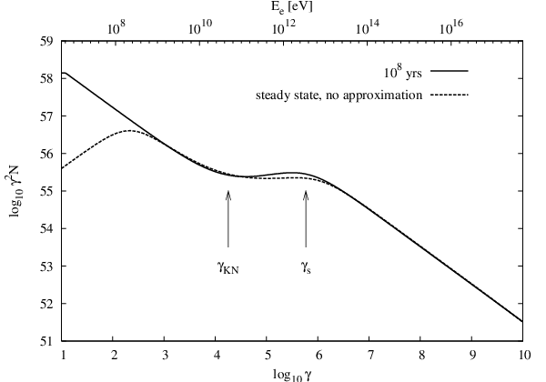
In this case it is straightforward to incorporate the general term for given by Eq. (16). In Fig. 2, we compare this solution with the time dependent solution obtained by using Eqs. (6) and (7) with the approximate cooling term given in Eq. (24). We take years, which is sufficiently large to allow a steady state to be achieved, and assume no particles are present initially, . In this figure, escape is neglected, , and the ratio of the energy density of the photon field to that of the magnetic field is . The remaining parameters are the same as in Fig. 1 Note that here, and in the following, we restrict our calculations to the case of a thermal distribution of target photons. The qualitative picture is similar to the case of a photon field following a power-law.
For , Coulomb losses harden the spectrum to . Since the time-dependent solution is based upon a “simplified” energy-loss term given in Eq. (23) neglecting the Coulomb energy losses, the two solutions deviate in this range. Between and , electrons cool predominantly via inverse Compton scattering in the Thomson limit. For values of , the drop in the inverse Compton scattering cross section in the Klein-Nishina regime leads to a spectral hardening until synchrotron losses become dominant for . The positions of and are indicated in Fig. 2. The slight deviation observed for is the result of the approximation used for given in Eqn. (21). From Fig. 2, it is obvious that (a) the approximation used to take the energy dependence of the inverse Compton scattering cross section into account follows quite well the exact calculation and (b) neglecting Coulomb losses mainly affects the low energy part of the spectrum.
3.2 Temporal evolution
The temporal evolution of for an arbitrary injection function can now be calculated. In the following we investigate the impact of the relevant parameters (). In order to demonstrate the effect of KN cooling on the temporal evolution, we plot in Fig. 3 the evolution of and as a function of time for two different temperatures ( K and K) which are representative for an environment dominated by hot stars or by re-processed emission from warm dust. For comparison, the evolution of and in the Thomson limit is depicted by thin lines. In both cases, the parameters have been chosen similar to the ones used above (G, eV cm-3 corresponding to , ) with and . The evolution of is dominated by slow cooling in the Thomson limit and therefore, the two lines are identical. For the high temperature environment (Fig. 3a), cools via synchrotron radiation until roughly 1 Myr, when the energy losses in the KN limit take over. Within a few hundred thousand years, the transition to Thomson-limit cooling takes place when . Qualitatively, the evolution of for a cooler photon field proceeds in a similar way (Fig. 3b). It is, however, important to note that the respective transitions occur much earlier. Whereas for K, synchrotron cooling prevails for about Myr, for K, Compton cooling in the KN regime is reached within a few hundred years.
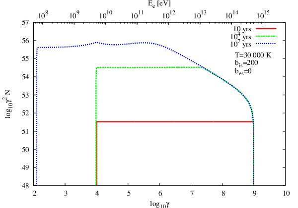
The effect on the temporal evolution of a particle distribution which is partially cooling via inverse Compton radiation in the KN limit, assuming continuous power-law electron injection with between and , neglecting escape losses () and with the environmental parameters described above is shown in Fig. 4. The solutions for , , and years, weighted with so that the injected spectrum appears constant, are compared with solutions found using expressions for the cooling valid in the Thomson limit (see Appendix B), which are depicted as thin lines.
The solutions for yrs (see also Fig. 3a) correspond to the case (the position of is marked by an arrow in Fig. 4). The solution taking KN effects into account shows a break such that for while for smaller , a slight deviation from the injection power-law can be observed which marks the onset of rapid energy loss in the KN regime. In the solution obtained in the Thomson limit, the break occurs at a smaller value of (see also Fig. 3a) which marks the transition from the uncooled part of the spectrum to the part which has already suffered from cooling. At the solution at a later time ( yrs), when , the flattened spectral shape presented earlier in the steady state solution (see Fig. 2), has already fully developed as a consequence of the large in the KN regime. The solution obtained in the Thomson limit and that obtained taking KN effects into account, agree with each other for , which marks the transition to cooling in the Thomson limit. Finally, for yrs, , and the further temporal evolution is well described in the Thomson limit.
In the next example, we consider a higher value of while keeping the same values for all other parameters as in the examples above. Fig. 5, shows for three different times: , , and years. The shape of the spectrum evolves, as expected, mainly due to synchrotron cooling for years. At later times (e.g., yrs), the spectrum shows a smooth transition between and at . For smaller values of , the spectrum remains almost flat, showing a slight peak at the position of . The overall shape of this evolved spectrum could, in principle, mimic the case of an uncooled spectrum up to TeV energies (depending on the value of ) with a softening at resembling a much younger source. Remarkably, for , the effect of cooling in KN is almost hidden when . For higher values of , a hard particle spectrum can be retained up to even higher values of than those shown here (see also next example).
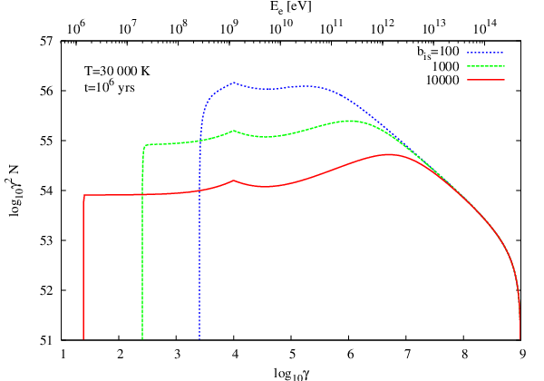
Changing the ratio of the photon and magnetic field energy densities () at fixed photon temperature influences the location of the transition between inverse Compton and synchrotron cooling. In Fig. 6, the effect of varying from values of 100 up to 104 is demonstrated. Increasing leads to more rapid cooling and a more pronounced spectral hardening as a result of inverse Compton cooling in the KN limit.
Finally, we consider the effect of particle escape via diffusive particle transport leaving a sphere with radius . In Fig. 7, the solution is shown for values of , , and at yrs (solid lines). For comparison, the solution of Appendix B in the Thomson limit is also shown (dashed lines). All other parameters are the same as in the previous example. As expected, the effect of escape losses leads to a reduction of total particle number. For escape losses are negligible, whereas for and , escape losses modify the solution considerably in comparison to the case of small . The solution taking KN effects into account shows a stronger relative suppression of particle numbers for than in the Thomson limit. This is a consequence of the fact that, in the KN case, radiative cooling is dominated by synchrotron losses for which implies that escape losses are relatively more important () than in the Thomson limit, where with . In general, when escape losses are important, the spectral features characteristic for cooling in the KN limit are suppressed, and the solution resembles that found in the Thomson limit. Asymptotically, for very large , radiative cooling is negligible and the two solutions converge.


4 Application to a stellar association: Westerlund 2
The discovery of VHE gamma-ray emission from young stellar associations like Westerlund 2 (Wd-2), Cyg OB2, and Berkeley 87 is providing first clear evidence that particle acceleration can occur in these systems. While the origin of the emission and the nature of the accelerated particles is not clear, it has been suggested that gamma-rays from stellar associations could be the decay product of neutral mesons in inelastic scattering of nuclei with the ambient medium (Torres et al. 2004; Bednarek 2007) or due to the excitation of giant resonances of nuclei by Doppler boosted UV photons (Anchordoqui et al. 2007b). Here, we calculate the broad band spectral energy distribution of Wd-2 at different stages of its evolution. The distance to this system is not very well constrained (Churchwell et al. 2004). A recent estimate places Wd-2 at kpc, with an age of Myrs, and a total mass of (Ascenso et al. 2007). While this distance estimate is based mainly on near infra-red photometry and colors, the spectroscopic investigation of the cluster and the light-curve of the binary system WR 20a has provided a larger distance estimate of kpc (Rauw et al. 2007). Another recent distance estimate is based upon the possible association of RCW 49 with a giant molecular cloud with a mass of at a kinematic distance of kpc (Dame 2007) For our calculations we adopt a distance of kpc and note that the larger distance would affect the total energetics, requiring a higher injection rate.
The angular extension, of the VHE gamma-ray emission region (Aharonian et al. 2007) implies a radial extension of . The total luminosity of the member stars of O-type has been estimated to be ergs s-1 (Rauw et al. 2007). However, it is well known that the number of UV photons emitted by the early cluster member stars is not sufficient to power the HII region RCW 49 in which Wd-2 is embedded. Based upon the estimates of Rauw et al. 2007, only % of the UV photons required to power RCW 49 can be attributed to known O stars. Therefore, the assumed luminosity of the early type stars is certainly a lower limit and the total luminosity could in fact reach values beyond ergs s-1. It is noteworthy, that the population of later type stars shows a rather flat projected spatial distribution even beyond a distance of pc (Ascenso et al. 2007) which would lead to a higher average energy density of the photon field. In addition to the stellar photons, re-processed emission from the dust present in Wd-2 and its surrounding will provide a contribution to the seed photon field for inverse Compton scattering which is however not included here and left for a more detailed modelling.
Taking into account just the total power emitted by the early type stars in the cluster, the average energy density of the hot photon field at a distance corresponding to the extension of the VHE gamma-ray source can be estimated as:
| (37) |
Based upon the extension of the VHE source of pc, eV cm-3. However, given the presence of additional (diffuse) UV photons implied by the ionisation state of RCW 49, we choose eV cm-3 as the average energy density and a temperature of K to characterise the target photon field. The magnetic field is set to G, placing it in approximate equipartition with the thermal energy density of the gas, assuming a source radius of pc. The injection rate is assumed to be constant in time with a total power of ergs s-1 following a power-law with between and . The required injection power can be compared, for example, with the total power injected by the stellar winds driven by the early type stars (mainly the Wolf-Rayet stars WR 20a&b) present in Wd-2 which has been estimated to be ergs s-1 (Rauw et al. 2007). If the emitting electrons are accelerated by these stellar winds, they must take roughly % of the kinetic power of the bulk flow.
In hadronic scenarios, on the other hand, the required efficiency is generally much larger, because of the relatively long cooling times involved. For example, inelastic proton-proton scattering producing , operates on a timescale of yrs ( denotes the ambient medium density), which is larger than the age of the accelerator, assuming this is limited to the maximum time that massive stars drive strong and fast stellar winds in their Wolf-Rayet phase (this lasts approximately, yrs, see also below). This implies that under most conditions, the efficiency required in hadronic models is close or larger than unity. A similar conclusion can be drawn for the case of gamma-ray production through photo-excitation of heavy nuclei, where the efficiency of acceleration of exclusively iron nuclei has to reach values in excess of (Anchordoqui et al. 2007a).
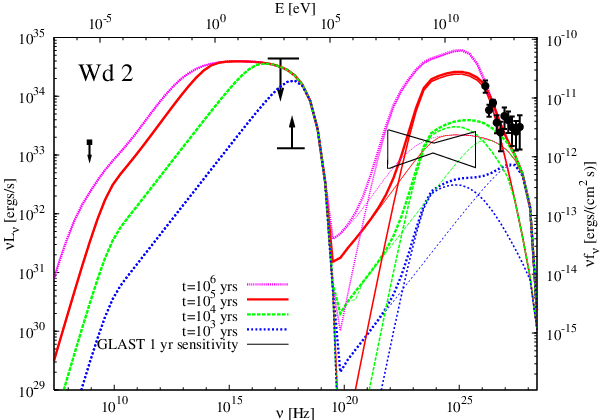
The electron distribution is computed for four different times , , , and years. The synchrotron and inverse Compton emissivities are calculated following the approach described in Appendix C and the resulting broad band spectral energy distribution (SED) is presented in Fig. 8. In addition to the UV photons from the early type stars, CMB photons are, of course, also present with an energy density . Although the energy loss due to inverse Compton scattering on these photons is negligible, they are nevertheless quite important for the total hard gamma-ray emission. This is because the inverse Compton scattering off UV photons is strongly suppressed, leading for sufficiently large to emissivities which are smaller than the contribution from scattering with CMB photons. We therefore include in the inverse Compton emissivity calculation the CMB photon field and show in Fig. 8, the total (heavy line width) inverse Compton emission as well as the contribution from UV photons (medium line width) and from CMB photons (thin line). It is interesting to note how the inverse Compton emission from the CMB photons dominates for young sources. With increasing age, the UV-related component at about TeV increases steadily until, after years — roughly the age of this stellar cluster — it exceeds the CMB-related contribution. This effect is due to the accumulation of electrons of Lorentz factor () within the source (see Fig. 5).
The model SED is compared in Fig.8 with VHE measurements (Aharonian et al. 2007) and with X-ray measurements Townsley et al. 2005 taken with Chandra (indicated as a lower limit) and earlier measurements taken with the Einstein X-ray telescope (Goldwurm et al. 1987) (indicated as an upper limit). Whereas the limited field of view of the Chandra observations may underestimate the total extended X-ray emission, the Einstein observations may overestimate the diffuse flux, because of the limited spatial resolution which does not allow the subtraction of the point sources present. In this figure we also show the total integrated radio flux of Jy at 843 MHz. This we consider as an upper limit which should not be exceeded by the non-thermal radio flux produced by the energetic electrons (Whiteoak & Uchida 1997). Overall, the model SED is in good agreement with the observations. The VHE energy spectrum is well reproduced for years, and the constraints from X-ray and radio measurements are not violated. It is interesting to note that for stars with , the Wolf-Rayet phase is expected to last up to roughly years (Maeder & Meynet 1987), which is consistent with the injection time required to match the data in this model. In contrast, an age of yrs would be too long for acceleration in a supernova remnant, a hypothesis which also has to contend with the fact that, so far, no indication for the presence of a supernova remnant associated with Wd-2 has been reported.
The predicted X-ray flux is quite close to the upper bound imposed by the Einstein measurements. However, it should be noted that this prediction is sensitive to the energy density in the target photon field — an increase by a factor of 2 in the energy density in the seed photon field (either from the late type stars and/or emission from dust) reduces the required injection power and, consequently, the predicted X-ray flux is also reduced by a factor of 2. We also indicate in Fig. 8 the one year flux sensitivity of the upcoming GLAST gamma-ray mission11 1 taken from www-glast.slac.stan.edu, official GLAST homepage. Our calculations predict that GLAST should easily detect the source. The combined energy spectrum of GLAST and H.E.S.S. would provide a broad band energy spectrum which in turn might allow one to infer, for example, the age of the source in the model scenario suggested here.
5 Conclusions
We have presented a method for computing the time-dependent electron distribution in the continuous energy loss limit for an arbitrary source function, under the assumptions of
- •
an isotropic electron distribution
- •
negligible ionization and Bremsstrahlung losses,
- •
time-independent energy losses by synchrotron radiation in a homogeneous magnetic field and
- •
by inverse Compton scattering off a spatially homogeneous mono-energetic or power-law energy distribution of target photons,
- •
an escape probability proportional to the particle energy, as expected for diffusion in the Bohm limit.
The key innovation of the model is that it utilises a simplified expression introduced by Moderski et al. 2005b for the inverse Compton scattering rate (including KN-effects) to construct explicit analytic expressions (see Appendix A) for the integrated cooling time (, Eq. 2)) and the integrated escape function (, Eq. (3)). This enables the electron distribution to be computed in a single quadrature.
The extension of this approach to include different energy dependencies of the escape probability would be relatively straightforward. However, the treatment of multiple and/or time-dependent target photon fields would probably require numerical evaluation of the functions and .
We have used this method to present an in-depth discussion of the properties of cooling electron distributions, and have identified features characteristic of cooling by inverse Compton scattering:
- 1.
The effect of “spectral ageing” observed in the Thomson limit is strongly modified. While in the Thomson limit, a well-defined spectral break changes position with time (cooling break), this spectral break is not evident anymore for , when KN effects are taken into account (see Fig. 4).
- 2.
- 3.
- 4.
The effect of particle escape modifies the observed energy spectra stronger for than for smaller values of which can lead to energy spectra resembling more the ones obtained in the Thomson limit (see Fig. 7).
We have illustrated our technique by applying it to high energy observations of the open stellar cluster Westerlund 2, and calculating the broad band emission spectrum. Comparing our results with the available observations, we have identified a consistent parameters set: , G, K, total injected power in electrons ergs s-1, distance=2.8 kpc, pc, , , . Although the uncertainty on the distance affects the values of some parameters (eg. , and total power), it is interesting to note that the suggested model of an electron accelerator embedded in the intense stellar radiation field which has been injecting a power-law type spectrum for the past few yrs, can account naturally for the observed gamma-ray spectrum, without violating the constraints derived from X-ray and radio observations. Furthermore, the rather long injection time favours acceleration in stellar winds of, for example, Wolf-Rayet stars over acceleration in supernova remnants. A leptonic scenario of gamma-ray production requires only a moderate fraction ( %) of the kinetic power of the stellar winds to be channelled into the acceleration of a non-thermal particle population. Hadronic models, on the other hand, need a rather high ambient gas density in order to keep the required efficiency below unity. The model presented here can be improved further by including a more realistic mixture of different temperature photon fields with different spatial extensions as observed in the vicinity of Wd-2 (including a dust component and later-type stars present in the system). However, it already makes testable order of magnitude predictions of the flux in the range accessible to the GLAST experiment.
Acknowledgements.
DH and KM acknowledge the support of the Eberhard Karls Universität Tübingen. This research has made use of NASA’s Astrophysics Data System.Appendix A Characteristic cooling and escape functions
The integrals in Eqs (25) and (26) can be rewritten as
| (38) | |||||
and
| (39) | |||||
where the indefinite integrals and can be expressed in terms of elementary functions for (negative) integer and half-integer values of .
In the case of black-body target photons, as well as for power-law photons with index , and , one has , and finds, for :
| (40) | |||||
where
,
,
,
,
,
,
and, for :
| (41) |
For the indefinite integral one finds, for :
| (42) | |||||
where
,
,
,
,
and, for :
| (43) |
In the case of a power-law distribution of target photons with , closed form expressions of the integrals can be found for the special cases and , corresponding to and , respectively. For :
| (44) |
| (45) |
whereas for one has for :
| (46) |
where
,
,
,
,
and, for :
| (47) |
Similarly, for the function we find, for :
| (48) |
where
,
,
and, finally, for :
| (49) |
Appendix B
For the case where accelerated particles start to inject from the central source at time with a power-law type finite energy spectrum:
| (50) |
undergoing synchrotron and inverse Compton losses in the Thomson regime: , and escaping from the system (with radius ) at a rate (see § 2.2), the solution of Eq. (1) splits into two branches,
depending on whether the maximum injected energy, has had enough time to “cool down” to a
value being smaller or larger than the minimum injected energy, .
If , then the solution reads:
| (51) |
If , one gets:
Appendix C Inverse Compton and synchrotron emissivities
The spectrum of photons scattered by an energetic electron from an isotropic photon gas which follows a differential photon number density has been derived e.g. by Blumenthal & Gould 1970 in the head-on collision approximation and is given by their Eqn.2.48:
| (53) |
with
| (54) |
and
| (55) |
The total inverse Compton spectrum from a distribution of electrons follows from the integration over and :
| (56) |
The emitted synchrotron power per unit frequency interval emitted by a single electron with pitch angle and magnetic field is given e.g. by Ginzburg & Syrovatskii 1964:
| (57) |
with the critical frequency:
| (58) |
and
| (59) |
A simple approximation of has been used for the calculations presented in this paper (see e.g. Melrose 1980):
| (60) |
This approximation provides a relative accuracy better than 1 per cent in the region of the maximum at , and still reasonable accuracy in the broad range of . The luminosity per unit frequency interval from an electron distribution is calculated by integration over :
| (61) |
We assume an isotropic magnetic field such that .
References
- Abdo et al. (2007) Abdo, A. A., Allen, B., Berley, D., et al. 2007, ApJ, 658, L33
- Aharonian et al. (2002) Aharonian, F., Akhperjanian, A., Beilicke, M., et al. 2002, A&A, 393, L37
- Aharonian et al. (2005a) Aharonian, F., Akhperjanian, A., Beilicke, M., et al. 2005a, A&A, 431, 197
- Aharonian et al. (2005b) Aharonian, F., Akhperjanian, A. G., Aye, K.-M., et al. 2005b, Science, 309, 746
- Aharonian et al. (2005c) Aharonian, F., Akhperjanian, A. G., Aye, K.-M., et al. 2005c, A&A, 442, 1
- Aharonian et al. (2007) Aharonian, F., Akhperjanian, A. G., Bazer-Bachi, A. R., et al. 2007, A&A, 467, 1075
- Albert et al. (2006) Albert, J., Aliu, E., Anderhub, H., et al. 2006, Science, 312, 1771
- Anchordoqui et al. (2007a) Anchordoqui, L. A., Beacom, J. F., Butt, Y. M., et al. 2007a, ArXiv e-prints, 706
- Anchordoqui et al. (2007b) Anchordoqui, L. A., Beacom, J. F., Goldberg, H., Palomares-Ruiz, S., & Weiler, T. J. 2007b, Physical Review Letters, 98, 121101
- Ascenso et al. (2007) Ascenso, J., Alves, J., Beletsky, Y., & Lago, M. T. V. T. 2007, A&A, 466, 137
- Bednarek (2007) Bednarek, W. 2007, ArXiv e-prints, 704
- Blumenthal (1971) Blumenthal, G. R. 1971, Phys. Rev. D, 3, 2308
- Blumenthal & Gould (1970) Blumenthal, G. R. & Gould, R. J. 1970, Reviews of Modern Physics, 42, 237
- Churchwell et al. (2004) Churchwell, E., Whitney, B. A., Babler, B. L., et al. 2004, ApJS, 154, 322
- Coppi (1992) Coppi, P. S. 1992, MNRAS, 258, 657
- Dame (2007) Dame, T. M. 2007, ArXiv e-prints, 707
- Dermer & Atoyan (2002) Dermer, C. D. & Atoyan, A. M. 2002, ApJ, 568, L81
- Felten & Morrison (1966) Felten, J. E. & Morrison, P. 1966, ApJ, 146, 686
- Ginzburg & Syrovatskii (1964) Ginzburg, V. L. & Syrovatskii, S. I. 1964, The Origin of Cosmic Rays (The Origin of Cosmic Rays, New York: Macmillan, 1964)
- Goldwurm et al. (1987) Goldwurm, A., Caraveo, P. A., & Bignami, G. F. 1987, ApJ, 322, 349
- Hinton & Aharonian (2007) Hinton, J. A. & Aharonian, F. A. 2007, ApJ, 657, 302
- Horns et al. (2007) Horns, D., Hoffmann, A. I. D., Santangelo, A., Aharonian, F. A., & Rowell, G. P. 2007, ArXiv e-prints, accepted for publication in A&A Letters, 705
- Jones (1965) Jones, F. C. 1965, Physical Review, 137, 1306
- Kardashev (1962) Kardashev, N. S. 1962, AZh, 39, 393
- Katarzyński et al. (2006) Katarzyński, K., Ghisellini, G., Svensson, R., & Gracia, J. 2006, A&A, 451, 739
- Khangulyan et al. (2007) Khangulyan, D., Hnatic, S., & Aharonian, F. 2007, Ap&SS, 212
- Kirk et al. (1999) Kirk, J. G., Ball, L., & Skjaeraasen, O. 1999, Astroparticle Physics, 10, 31
- Krawczynski et al. (2002) Krawczynski, H., Coppi, P. S., & Aharonian, F. 2002, MNRAS, 336, 721
- Kusunose & Takahara (2005) Kusunose, M. & Takahara, F. 2005, ApJ, 621, 285
- Lightman & Zdziarski (1987) Lightman, A. P. & Zdziarski, A. A. 1987, ApJ, 319, 643
- Maeder & Meynet (1987) Maeder, A. & Meynet, G. 1987, A&A, 182, 243
- Mastichiadis & Kirk (1997) Mastichiadis, A. & Kirk, J. G. 1997, A&A, 320, 19
- Melrose (1980) Melrose, D. B. 1980, Plasma astrophysics: Nonthermal processes in diffuse magnetized plasmas. Volume 2 - Astrophysical applications (New York, Gordon and Breach Science Publishers, 1980. 430 p.)
- Moderski et al. (2005a) Moderski, R., Sikora, M., Coppi, P. S., & Aharonian, F. 2005a, MNRAS, 364, 1488
- Moderski et al. (2005b) Moderski, R., Sikora, M., Coppi, P. S., & Aharonian, F. 2005b, MNRAS, 363, 954
- Murata et al. (2003) Murata, K., Tamaki, H., Maki, H., & Shibazaki, N. 2003, PASJ, 55, 473
- Neronov & Chernyakova (2006) Neronov, A. & Chernyakova, M. 2006, ArXiv Astrophysics e-prints
- Rauw et al. (2007) Rauw, G., Manfroid, J., Gosset, E., et al. 2007, A&A, 463, 981
- Stawarz & Kirk (2007) Stawarz, Ł. & Kirk, J. G. 2007, ApJ, 661, L17
- Sturner et al. (1997) Sturner, S. J., Skibo, J. G., Dermer, C. D., & Mattox, J. R. 1997, ApJ, 490, 619
- Tang & Wang (2005) Tang, S. & Wang, Q. D. 2005, ApJ, 628, 205
- Torres et al. (2004) Torres, D. F., Domingo-Santamaría, E., & Romero, G. E. 2004, ApJ, 601, L75
- Townsley et al. (2005) Townsley, L., Feigelson, E., Montmerle, T., et al. 2005, in X-Ray and Radio Connections (eds. L.O. Sjouwerman and K.K Dyer) Published electronically by NRAO, http://www.aoc.nrao.edu/events/xraydio Held 3-6 February 2004 in Santa Fe, New Mexico, USA, (E3.04) 10 pages
- Völk (2006) Völk, H. J. 2006, in IAU Symposium, Vol. 230, Populations of High Energy Sources in Galaxies, ed. E. J. A. Meurs & G. Fabbiano, 95–102
- Whiteoak & Uchida (1997) Whiteoak, J. B. Z. & Uchida, K. I. 1997, A&A, 317, 563
- Zdziarski (1989) Zdziarski, A. A. 1989, ApJ, 342, 1108