Entanglement Distribution in Pure-State Quantum Networks

Sébastien Perseguers Email: sebastien.perseguers@mpq.mpg.de Affiliation: Max-Planck–Institut für Quantenoptik, Hans-Kopfermann-Str. 1, D-85748 Garching, Germany J. Ignacio Cirac Affiliation: Max-Planck–Institut für Quantenoptik, Hans-Kopfermann-Str. 1, D-85748 Garching, Germany Antonio Acín Affiliation: ICFO-Institut de Ciències Fotòniques, Mediterranean Technology Park, E-08860 Castelldefels (Barcelona), Spain
ICREA-Institució Catalana de Recerca i Estudis Avançats, Lluis Companys 23, 08010 Barcelona, Spain Maciej Lewenstein Affiliation: ICFO-Institut de Ciències Fotòniques, Mediterranean Technology Park, E-08860 Castelldefels (Barcelona), Spain
ICREA-Institució Catalana de Recerca i Estudis Avançats, Lluis Companys 23, 08010 Barcelona, Spain Jan Wehr Affiliation: Department of Mathematics, The University of Arizona, Tucson, AZ 85721-0089, USA

October 31, 2007

Abstract

We investigate entanglement distribution in pure-state quantum networks. We consider the case when non-maximally entangled two-qubit pure states are shared by neighboring nodes of the network. For a given pair of nodes, we investigate how to generate the maximal entanglement between them by performing local measurements, assisted by classical communication, on the other nodes. We find optimal measurement protocols for both small and large 1D networks. Quite surprisingly, we prove that Bell measurements are not always the optimal ones to perform in such networks. We generalize then the results to simple small 2D networks, finding again counter-intuitive optimal measurement strategies. Finally, we consider large networks with hierarchical lattice geometries and 2D networks. We prove that perfect entanglement can be established on large distances with probability one in a finite number of steps, provided the initial entanglement shared by neighboring nodes is large enough. We discuss also various protocols of entanglement distribution in 2D networks employing classical and quantum percolation strategies.

pacs

03.67.-a, 03.67.Bg

I Introduction

Quantum Networks Cirac et al. 1997; Boozer et al. 2007 play a key role in quantum information processing. In such networks, quantum states can be prepared initially and shared between neighboring nodes (or stations), i.e. entanglement can be generated, and this resource is then to be used for quantum communication Ekert 1991; Bennett et al. 1993, or distributed quantum computation Cirac et al. 1999 involving arbitrary nodes of the network. One of the main tasks is then to design protocols that use the available quantum correlations to entangle two nodes of the network, and to optimize these protocols in terms of final entanglement and probability of success.

A set of quantum repeater stations, for instance (see Fig. 1a), can be considered as a 1D quantum network, where the aim is to establish quantum communication over large distances Briegel et al. 1998; Dür et al. 1999; Childress et al. 2005; Hartmann et al. 2007. It is well known that the simple entanglement swapping Zukowski et al. 1993 procedure can achieve this goal, but (except for the unrealistic case of perfect resources and operations) the probability of obtaining entanglement between the end-nodes of such a network decays exponentially with the number of repeaters. This problem can be overcome by the more sophisticated quantum repeaters protocols Briegel et al. 1998; Dür et al. 1999; Childress et al. 2005; Hartmann et al. 2007 which intersperse “connection steps” (entanglement swapping) with purification steps and require only polynomial decay, thus opening the way for feasible long-distance quantum communication.

In two-dimensional or higher dimensional lattices of large size, a perfect connection between any two nodes is possible with a probability that is strictly greater than zero, even with imperfect resources. This can be achieved by the so-called classical and quantum percolation strategies Acín et al. 2007, in which initially, or after some preparatory measurements, respectively, one converts all bonds into singlets with a probability $p$ . This result is very encouraging, but remains of little use for finite and small networks Keller et al. 2004; Eisaman et al. 2005. The aim of the present paper is twofold: first, we investigate and derive optimal local measurement protocols for simple networks of finite size. In particular, we consider certain 1D and 2D networks of nodes that consist of $z$ qubits, where $z$ is the number of neighbours. Neighboring nodes share partially entangled pure states. We apply then local quantum operations to the nodes, assuming that these operations are noiseless. We first address the question of optimal entanglement propagation, or in another words entanglement swapping, in small networks consisting of three or four nodes only. The insights obtained for these simple situations are then used as building blocks for larger 1D and 2D quantum networks, as well as networks with hierarchical geometry.

Our second aim is to discuss examples of hierarchical “diamond” and “tree” lattices in which perfect entanglement on arbitrary large distances can be achieved in a finite number of steps (measurements). Provided that sufficiently large but not necessarily maximal entanglement is present, we can convert connections along a given line into prefect singlets. Finally, we consider various kinds of percolation strategies: the one presented in Ref. Acín et al. 2007, which employs a change in the lattice connectivity due to quantum measurements, and a different one in a triangular lattice, where the optimal singlet conversion strategy is used. Both of these protocols essentially demonstrate that the quantum percolation thresholds are lower than their classical counterparts. Equally interesting we propose to use the optimal singlet conversion strategy to transform a square lattice into two independent square lattices of doubled size, for which the percolation probability is larger than in the original lattice.

Outline

In Section II we fix the notation and define the figures of merit used for evaluating the measurements efficiency: the concurrence (C), the so-called worst case entanglement (WCE) and the singlet conversion probability (SCP). In Sec. III we describe the strategies maximizing these quantities for some 1D networks, starting from a simple one-repeater configuration, consisting of two bonds with two imperfectly entangled pairs on them. Interestingly, there exists a strategy that conserves the averaged singlet conversion probability Bose et al. 1999; the protocols however does not scale with the number of repeaters, as expected. The second subsection of Sec. III deals with the problem of two repeaters, that is three bonds. Here the optimization of the SCP is much more complex: in some conditions we obtain that the optimal measurements do not correspond to a Bell measurement, i.e. von Neumann measurements in a Bell basis of orthonormal maximally entangled states. This result is somewhat analogue to the recent result by Modławska and Grudka Modławska and Grudka 2007, who have demonstrated that non-maximally entangled states can be better for the realization of multiple linear optical teleportation in the scheme of Knill, Laflamme and Milburn Knill et al. 2001. The last part of this section deals with large 1D network (i.e. in the limit of infinite size network). Here we prove that the probability of establishing entanglement over large distances decays exponentially. We present optimal strategies for the concurrence and the WCE, and upper bounds for the SCP.

In Sec. IV we turn to the simplest small network in 2D: a square. We obtain similar results as in the case of two repeaters in 1D, indicating that Bell measurements not always provide the best protocol. In Sec. V we apply the results of previous sections to networks of large size and hierarchical geometry, that is, lattices that iterate certain geometric structures, so that at each level of iterations the number of nodes, or the number of neighbors changes. We consider two kinds of hierarchical lattices: first we discuss the so-called “diamond” lattice, for which we prove that for sufficiently large initial entanglement, one can establish perfect entanglement on large scales (i.e. some lower levels of iteration) in finite number of steps. A somewhat simpler result holds for the simplest possible double Cayley tree lattice, in which in each step of iteration each bond branches into two. For such lattices, if the initial entanglement is large enough, perfect entanglement can be established at each level of iteration.

Finally, in Sec. VI we consider genuine 2D lattices. First, using similar method as in Sec. V we show that for a sufficiently broad strip of a square lattice, we can convert connections of a given line along the strip into a line of perfect singlets, provided, of course, that initially an imperfect, but sufficiently large entanglement is present. Second we reconsider percolation strategies and discuss the example of hexagonal lattice with double bonds from Ref. Acín et al. 2007, and a triangular lattice with variable bonds. In the first of these examples quantum measurements lead to local reduction of the SCP, but change the geometry of the lattice, increasing its connectivity and thus the classical percolation threshold. In the second example we use a protocol optimizing the SCP to transform the original lattice to a new one with the same geometry, but with a higher probability $p$ of getting a singlet on a bond. Similarly, we discuss a different type of strategy, where by using the optimal singlet conversion protocol we transform a square lattice into two independent square lattices with the same mean SCP as the initial one. We prove that the classical probability of connecting a pair of neighboring points in the initial lattice (two neighboring point from the two lattices) to another such pair is strictly larger for the case of two lattices. We conclude then in Sec. VII.

II Preliminaries: Notation and Basic Notions

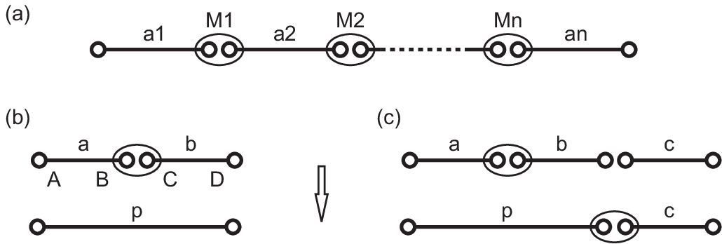
Refer to caption — Figure 1: Notation and examples of 1D networks: (a) the standard quantum repeater scenario; (b) entanglement swapping; (c) a two-repeater system.

A pure state of two qubits is represented by a solid line in the figures and is written (except when specified) as

\,|\alpha\rangle=\sqrt{\alpha_{0}}\,|00\rangle+\sqrt{\alpha_{1}}\,|11\rangle,

(1)

where $\alpha_{0}+\alpha_{1}=1$ and $\alpha_{0}\geq\alpha_{1}$ (it is assumed that local basis rotations are performed whenever necessary for the states to be written in that way). This defines the Schmidt decomposition of a pure state of two qubits, while $\alpha_{0}$ and $\alpha_{1}$ are their Schmidt coefficients.

II.0.1 Entanglement Swapping

A basic operation for propagating entanglement over larger distances is the so called “entanglement swapping”, see Fig. 1b. A POVM is described by $n$ positive operators $E_{m}\in M_{4}(\mathbb{C})$ satisfying the completeness relation $\sum_{m=1}^{n}E_{m}=\openone_{4}$ . Let

\rho_{m}=\tr_{BC}\big((\openone_{2}\otimes E_{m}\otimes\openone_{2})\,\,|\alpha\beta\rangle\negmedspace\langle\alpha\beta|\,\big)

be the resulting state of the measurement $M$ , which occurs with a probability $p_{m}=\tr(\rho_{m})$ . We consider in that paper projective measurements only, i.e. $n=4$ and $E_{m}=\,|u_{m}\rangle\negthinspace\langle u_{m}|\,$ for some normalized state $\,|u_{m}\rangle$ . For such measurements the smallest Schmidt coefficient of $\rho_{m}$ is $\lambda_{m}=\min\{\eig(\widetilde{\rho}_{m})\}/p_{m}$ , where $\widetilde{\rho}_{m}=\tr_{A}(\rho_{m})$ , or equivalently

\lambda_{m}=\frac{1}{2}\bigg(1-\sqrt{1-\frac{4\det(\widetilde{\rho}_{m})}{p_{m}^{2}}}\bigg).

(2)

Considering the following map from $\mathbb{C}^{2}\otimes\mathbb{C}^{2}$ to $M(\mathbb{C},2)$ :

\,|a\rangle=\sum_{i,j=0}^{1}a_{ij}\,|ij\rangle\quad\mapsto\quad\widehat{a}=\begin{pmatrix}a_{00}&a_{01}\\ a_{10}&a_{11}\end{pmatrix},

(3)

one can show that $\widetilde{\rho}_{m}$ is now equal to $X_{m}X_{m}^{\dagger}$ , with $X_{m}=\widehat{\alpha}\,\widehat{u}_{m}\,\widehat{\beta}$ .
The concurrence of a state $\varphi$ is by definition $C(\varphi)\equiv 2\,|\det(\widehat{\varphi})|$ . Therefore, the concurrence $C_{m}$ , the smallest Schmidt coefficient $\lambda_{m}$ and the outcome probability $p_{m}$ are explicitly given by


$\displaystyle C_{m}$	$\displaystyle=\frac{2\,\|\det(X_{m})\|}{p_{m}}=\frac{\sqrt{\alpha_{0}\alpha_{1}\beta_{0}\beta_{1}}}{p_{m}}\,C(u_{m}),$	(4a)
$\displaystyle\lambda_{m}$	$\displaystyle=\frac{1}{2}\left(1-\sqrt{1-C_{m}^{2}}\right),$	(4b)
$\displaystyle p_{m}$	$\displaystyle=\sum_{i,j=0}^{1}\alpha_{i}\beta_{j}\,\|\widehat{u}_{m,ij}\|^{2}.$	(4c)

We now turn to Bell measurements. Starting from the computational basis $\{\,|0\rangle,\,|1\rangle\}$ of a single qubit, we define the new orthonormal basis $\{\,|\negmedspace\uparrow\rangle,\,|\negmedspace\downarrow\rangle\}$

\begin{pmatrix}\,|\negmedspace\uparrow\rangle\\ \,|\negmedspace\downarrow\rangle\end{pmatrix}=U\begin{pmatrix}\,|0\rangle\\ \,|1\rangle\end{pmatrix},\quad U\in\mathcal{U}(2),

(5)

and the Bell vectors

\,|\Phi^{\pm}\rangle=\frac{\,|\negmedspace\uparrow\uparrow\rangle\pm\,|\negmedspace\downarrow\downarrow\rangle}{\sqrt{2}}\quad\text{and}\quad\,|\Psi^{\pm}\rangle=\frac{\,|\negmedspace\uparrow\downarrow\rangle\pm\,|\negmedspace\downarrow\uparrow\rangle}{\sqrt{2}}.

(6)

Two specific bases play a key role in this paper: the computational or “ZZ” basis, where the vectors $\,|\negmedspace\uparrow\rangle$ and $\,|\negmedspace\downarrow\rangle$ for both qubits are the eigenvectors of the Pauli matrix $\sigma_{z}$ , and the “XZ” basis, where the first basis is chosen as being the eigenvectors of $\sigma_{x}$ . Although we could in principle parameterize the Bell states in that way, calculations are much easier and clearer in the “magic basis” defined as Hill and Wootters 1997

(\widehat{\Phi}_{1},\,\widehat{\Phi}_{2},\,\widehat{\Phi}_{3},\,\widehat{\Phi}_{4})=(\openone_{2},\,-i\sigma_{z},\,i\sigma_{y},\,-i\sigma_{x})\,|\Phi^{+}\rangle,

(7)

which is nothing but the usual Bell basis with some specific phases. In this basis, the concurrence of a state $\,|\mu\rangle=\sum_{i=1}^{4}\mu_{i}\,|\Phi_{i}\rangle$ simply reads $C(\mu)=\big|\sum_{i=1}^{4}\mu_{i}^{2}\big|$ . It follows that the coefficients $\mu_{i}$ of a Bell state (whose concurrence is 1 by definition) have all the same phase; hence we can choose them as being real. Let a set of four such states $\{\mu_{m}\}$ , so that the matrix $(\mu_{m,i})$ belongs to $\mathcal{SO}(4)$ . Then the probabilities given in Eq. (4c) read

p_{m}=p_{\min}\left(\mu_{m,1}^{2}+\mu_{m,2}^{2}\right)+p_{\max}\left(\mu_{m,3}^{2}+\mu_{m,4}^{2}\right),

(8)

with

p_{\min}=\frac{\alpha_{0}\beta_{1}+\alpha_{1}\beta_{0}}{2}\quad\text{and}\quad p_{\max}=\frac{\alpha_{0}\beta_{0}+\alpha_{1}\beta_{1}}{2}.

(9)

We emphasize the fact that (given two states $\alpha$ and $\beta$ ), the outcome probabilities completely characterize a Bell measurement, since $\lambda_{m}$ depends only on $p_{m}$ for $C(u_{m})=1$ , see Eq. (4).

II.0.2 Figures of Merit

We describe here three figures of merit used to evaluate the usefulness of an entanglement swapping protocol: the concurrence, the singlet conversion probability (SCP) and the worst-case entanglement (WCE). All these figures of merit take value in the interval $[0,1]$ .

Concurrence

The average concurrence of a measurement $M$ is defined as

C_{M}=\sum_{m}p_{m}\,C_{m},

(10)

where $C_{m}$ is the concurrence of the outcome $m$ .

WCE

The idea of the WCE is to find a measurement optimizing the entanglement for all its outcomes. Taking the smallest Schmidt coefficient as the entanglement measure we define the WCE as

W_{M}=2\,\underset{m}{\min}\{\lambda_{m}\}.

(11)

SCP

We consider here the probability of conversion of a given state into a perfect singlet. A result of majorization theory Vidal 1999; Nielsen and Vidal 2001 tells us that a state $\,|\alpha\rangle$ (1) can be converted into a singlet by LOCC with maximal probability $2\,\alpha_{1}$ ; this is the “Procrustean method” of entanglement concentration described in Bennett et al. 1996. We define the average SCP for a measurement $M$ as

S_{M}=2\sum_{m}p_{m}\,\lambda_{m},

(12)

where $\lambda_{m}$ is the smallest Schmidt coefficient of the outcome $m$ . Since this figure of merit is used for different systems, we sometimes use the following notation for clarity:

S_{M}^{(N)}(\alpha_{1,0},\,\alpha_{2,0},\,\ldots,\,\alpha_{N+1,0}),

where $N$ means the number of repeaters of a 1D chain consisting of $N+1$ states $\alpha_{1},\,\alpha_{2},\,\ldots,\,\alpha_{N+1}$ , as depicted in Fig. 1a.

III 1D Networks

Before studying the two-dimensional networks, it is worth looking at systems made of one or two repeaters only. In fact, some interesting properties of these small systems can then be used in more elaborated strategies for larger networks. For instance, the important fact that the SCP does not decrease after one measurement (§III.1.3) allows one to get better results for the percolation on honeycomb lattices Acín et al. 2007. Another important and surprising result is that Bell measurements are not, in general, the measurements that maximize the SCP (§III.2.2), although they are the best ones for the average concurrence and the WCE. Previous results on 1D networks can also be found in Refs. Bose et al. 1998; Hardy and Song 2000.

III.1 One Repeater

We consider in this section a system consisting of two states $\alpha$ and $\beta$ joined by a single repeater, see Fig. 1b. We first prove a general statement on Bell measurements, and then describe the measurements that maximize our three figures of merit.

III.1.1 Bell Measurements and Outcome Probabilities

The following result is very useful when trying to maximize the SCP over the set of Bell measurements (the proof is given in App. A):

Result 1.

Outcome probabilities for a one-repeater Bell measurement

Let $\{x_{m}\}$ be four real numbers that add up to one and that lie in the interval $[p_{\min},\,p_{\max}]$ . Then there exists a Bell measurement whose outcome probabilities $p_{m}$ are equal to $x_{m}$ .

III.1.2 Maximizing the Concurrence and the WCE

It is clear from Eqs. (4a, 10) that any Bell measurement, i.e. $C(u_{m})=1\;\forall\,m$ , maximizes the average concurrence, and therefore

C_{\max}=2\sqrt{\alpha_{0}\alpha_{1}\beta_{0}\beta_{1}}.

(13)

The result of the maximization of the WCE is summarized in the following result:

Result 2.

Best WCE strategy for one repeater

The maximum value of $W$ for a one-repeater system is reached by the Bell measurement in the XZ basis, with

$W_{\max}=W_{\text{XZ}}=1-\sqrt{1-16\,\alpha_{0}\alpha_{1}\beta_{0}\beta_{1}}.$ (14)

Proof.

(By contradiction). The Bell states $\,|u_{m}\rangle$ in the XZ basis are given by the columns of the matrix

M_{\text{XZ}}=\frac{1}{2}\begin{pmatrix}-1&1&1&1\\ 1&-1&1&1\\ 1&1&-1&1\\ 1&1&1&-1\end{pmatrix},

hence $p_{m}=1/4$ and $2\lambda_{m}=1-\sqrt{1-16\,\alpha_{0}\alpha_{1}\beta_{0}\beta_{1}}\;\forall\,m$ . Now suppose that there exists a measurement $M$ described by the set $\left\{E_{m}=\,|u_{m}\rangle\negthinspace\langle u_{m}|\,\right\}_{m=1}^{n}$ , with $n\geq 4$ , such that $W_{M}>W_{\text{XZ}}$ . Then each $\lambda_{m}$ has to be strictly greater than the smallest Schmidt coefficient of the outcomes in the XZ basis. Thus, from Eq. (2)

\det(\widetilde{\rho}_{m})>p_{m}^{2}\,4\,\alpha_{0}\alpha_{1}\beta_{0}\beta_{1}\quad\forall\,m.

(15)

Since $\det(\widetilde{\rho}_{m})=\alpha_{0}\alpha_{1}\beta_{0}\beta_{1}\,|\det(\widehat{u}_{m})|^{2}$ , the summation over $m$ of the square root of Eq. (15) yields

\sum_{m=1}^{n}|\det(\widehat{u}_{m})|>2.

(16)

But the concurrence of a (normalized) state is smaller or equal than one, hence $2\,|\det(\widehat{u}_{m})|\leq\|u_{m}\|^{2}$ . Moreover, taking the trace of the completeness relation for the operators $E_{m}$ implies $\sum_{m=1}^{n}\|u_{m}\|^{2}=4$ . Therefore $\sum_{m=1}^{n}|\det(\widehat{u}_{m})|\leq 2$ , which is in contradiction with Eq. (16) and concludes the proof. $\square$

III.1.3 Maximizing the SCP

The following result gives the maximum value of the SCP for one entanglement swapping step:

Result 3.

Best SCP strategy for one repeater

The measurement that maximizes $S$ for a one-repeater configuration is the Bell measurement in the ZZ basis, and

$S_{\max}=S_{\text{ZZ}}=2\,\min\{\alpha_{1},\beta_{1}\}.$ (17)

Proof.

Two kinds of outcomes appear when performing a Bell measurement in the computational basis: two of the outcome probabilities are equal to $p_{\max}$ , while the other two are equal to $p_{\min}$ . Putting these values into Eq. (4) one finds the corresponding smallest Schmidt coefficients:

\lambda(p_{\max})=\frac{\alpha_{1}\beta_{1}}{2\,p_{\max}},\quad\lambda(p_{\min})=\frac{\min\{\alpha_{0}\beta_{1},\,\alpha_{1}\beta_{0}\}}{2\,p_{\min}},

(18)

whence $S_{\text{ZZ}}=2\,\min\{\alpha_{1},\beta_{1}\}$ . Consider now that we are allowed to perform some arbitrary unitary not only on $BC$ , but on $ABC$ . We are in presence of a bipartite system, and results of majorization theory apply: the SCP of this system is at most $2\,\beta_{1}$ . A similar construction for qubits $B$ , $C$ and $D$ tells us that the SCP is at most $2\,\alpha_{1}$ , so that the final SCP cannot exceed twice the minimum of $\alpha_{1}$ and $\beta_{1}$ . $\square$

Remark

Setting $\alpha=\beta$ , one sees that the SCP does not decrease after one entanglement swapping; this is the “conserved entanglement” described in Bose et al. 1999.

III.2 Two Repeaters

We consider a system of three states on which we perform two consecutive entanglement swappings, as shown in Fig. 1c, and we describe the measurements that maximize the three figures of merit.

III.2.1 Maximizing the Concurrence and the WCE

The maximization of these two figures of merit is trivial for a two-repeater configuration once one knows the results for the one-repeater system. First, any Bell measurement maximizes the average concurrence of the results of the two measurements. This will be generalized and proved for any number of repeaters in §III.3.1. Then, in order to maximize the WCE, we simply have to perform XZ measurements at both repeaters. In fact, if we perform any other measurement on the first repeater, then at least one resulting state $\varphi_{m}$ will be less entangled than the XZ results, and this reflects on the WCE of the second measurement (which has to be a Bell measurement in the XZ basis from Result 2).

III.2.2 Maximizing the SCP

After the first measurement, we get four resulting states $\,|\varphi_{m}\rangle$ with probabilities $p_{m}$ . From Result 3 we know that for any outcome, the second measurement has to be done in the ZZ basis. Hence, we have to find the first measurement $M$ that maximizes

S_{M}^{(2)}(\alpha_{0},\,\beta_{0},\,\gamma_{0})=2\,\sum_{m}p_{m}\,\min\{\varphi_{m,1},\,\gamma_{1}\}.

(19)

We first maximize this quantity over the set of Bell measurements (which, as we will see, leads to the best strategy for a large range of entangled states $\alpha$ , $\beta$ and $\gamma$ ), and then we present some numerical results showing that non-Bell measurements sometimes provide better results.

Bell Measurements

We fix the states $\alpha$ , $\beta$ and $\gamma$ and we consider the SCP as a function of the outcome probabilities only:

S(\{p_{m}\})=\sum_{m}\min\{f(p_{m}),\,g(p_{m})\}\equiv\sum_{m}h(p_{m}),

(20)

where $f(p)=2\gamma_{1}p$ and $g(p)=p-\sqrt{p^{2}-\alpha_{0}\alpha_{1}\beta_{0}\beta_{1}}$ . One can show that $g^{\prime}(p)<0$ and $g^{\prime\prime}(p)>0$ $\forall\,p\in[p_{\min},\,p_{\max}]$ . A typical plot of $h(p)$ is shown in Fig. 2, and the value $p^{*}$ at which the functions $f$ and $g$ cross each other is

p^{*}=\frac{1}{2}\sqrt{\frac{\alpha_{0}\alpha_{1}\beta_{0}\beta_{1}}{\gamma_{0}\gamma_{1}}}.

(21)

It is sufficient to maximize the function over the possible probability distributions, since Result 1 insures the existence of a Bell measurement leading to this optimal distribution; we recall that the probabilities have to be chosen in the interval $[p_{\min},p_{\max}]$ . Let us give two necessary conditions that have to be satisfied by the best probability distribution (they can be proven rigorously, but a look at Fig. 2 may be clearer):

•

if the set $\{p_{m}\}$ maximizes $S$ , then all probabilities lie either to the left of $p^{*}$ or to its right. In fact, suppose for example that $p_{1}+2\varepsilon<p^{*}<p_{2}-2\varepsilon$ , and choose $\tilde{p}_{1}=p_{1}+\varepsilon$ and $\tilde{p}_{2}=p_{2}-\varepsilon$ (with $0<\epsilon\ll 1$ as it should be). The constraints on these new probabilities are clearly satisfied if it was the case before, and a better SCP has been found.
•

if $p_{1}$ and $p_{2}$ are such that $p^{*}+2\varepsilon<p_{1}\leq p_{2}<p_{\max}-2\varepsilon$ , then the choice $\tilde{p}_{1}=p_{1}-\varepsilon$ and $\tilde{p}_{2}=p_{2}+\varepsilon$ gives rise to a strictly greater SCP (this comes from the convexity of $g$ ).

It is now simple to maximize the SCP of two repeaters, and one sees that the value $p^{*}$ , with respect to $p_{\min}$ and $p_{\max}$ , plays a crucial role in the choice of the best probability distribution. In fact, we have to distinguish four distinct cases; see results in Tab. 1. We notice that ZZ measurements lead to the maximum SCP whenever $p^{*}\leq p_{\min}$ , while the XZ ones are the best strategy for $p^{*}\geq 1/4$ . So far, we have maximized the SCP for two repeaters supposing that the first measurement was to be done on the states $\alpha$ and $\beta$ . But what happens if we start from the right side? It appears that the maximum SCP depends, in general, on the order of the measurements and that performing the first measurement where the states are more entangled yields better results.

value of $p^{*}$	$\{p_{m}\}$ maximizing $S^{(2)}$
^\| $p^{*}\leq p_{\min}$	$\{p_{\min},\,p_{\min},\,p_{\max},\,p_{\max}\}$
^\| $p_{\min}\leq p^{*}\leq(1-p_{\max})/3$	$\{p^{},\,p^{},\,p_{\max},\,1-2p^{*}-p_{\max}\}$
^\| $(1-p_{\max})/3\leq p^{*}\leq 1/4$	$\{p^{},\,p^{},\,p^{},\,1-3p^{}\}$
^\| $p^{*}\geq 1/4$	$\{1/4,\,1/4,\,1/4,\,1/4\}$

Table 1: Maximization of

S^{(2)}

over Bell measurements, see text for details.

General Measurements (Numerical Results)

The question is to check if some non-Bell measurements yield a better SCP than the results of the last paragraph. Since the concurrence of the states used for entanglement swapping can now take any value between 0 and 1, we cannot consider $S$ as a function of the outcome probabilities only. But for a fixed concurrence $C<1$ one sees that

\bar{g}(C,\,p)\equiv p-\sqrt{p^{2}-\alpha_{0}\alpha_{1}\beta_{0}\beta_{1}\,C^{2}}<g(p)\quad\forall\,p.

Writing the corresponding variables of non-Bell measurements with a bar, we have that $\bar{p}^{*}<p^{*}$ and $\bar{g}(C,\,\bar{p}^{*})<g(p^{*})$ . Therefore, one can check that Bell measurements are indeed the best ones, except, possibly, when $p_{\min}\leq p^{*}\leq(1-p_{\max})/3$ . The key fact about Bell measurements in that case is that we cannot chose three outcome probabilities to lie on $p^{*}$ , since the fourth one would be greater than $p_{\max}$ . But the range of possible outcome probabilities depends on the concurrence: for example, from Eq. (4c) and for $C(u_{m})=0$ , we have that $\bar{p}_{m}\in[\alpha_{1}\beta_{1},\,\alpha_{0}\beta_{0}]$ , or more generally

\bar{p}_{m}\in[\bar{p}_{\max},\,\bar{p}_{\min}]\supseteq[p_{\max},\,p_{\min}].

(22)

Hence, and this is confirmed by numerical results, a better strategy is to perform a measurement such that three outcomes probabilities are equal to $\bar{p}^{*}$ , and that the concurrences of the states are the largest ones satisfying $\bar{p}_{\max}=1-3\,\bar{p}^{*}$ . Our numerical evidence shows that Bell measurements do not always maximize the SCP, see Fig. 3.

III.3 Large 1D Chains

We consider the system of Fig. 1a that consists of $N$ repeaters joining $N+1$ states. For simplicity, we choose the states $\alpha_{i}$ as being identical: $\,|\alpha_{i}\rangle=\,|\varphi\rangle\;\forall\,i$ . We show in this section which strategies yield the optimal solution for the concurrence and the WCE, and for the SCP we give an upper bound to its maximum value and some results for XZ and ZZ measurements.

III.3.1 Maximizing the Concurrence and the WCE

A direct generalization of Eq. (4a) for $N$ repeaters yields for the concurrence Verstraete et al. 2004:

C^{(N)}=\sum_{\{m_{i}\}}2\,|\det\left(X_{\{m_{i}\}}\right)|,

(23)

where $X_{\{m_{i}\}}=\widehat{\varphi}\,\widehat{u}_{m_{1}}\,\widehat{\varphi}\ldots\widehat{u}_{m_{N}}\,\widehat{\varphi}$ , and the states $\,|u_{m_{i}}\rangle$ are associated with the measurement result $m_{i}$ of the $i$ -th repeater. Then the maximization of $C^{(N)}$ reads

\underset{M}{\max}\big\{C^{(N)}\big\}=|\det(\widehat{\varphi})|^{N+1}\ \max_{M}\Big\{\sum_{\{m_{i}\}}2^{N+2}\\ \Big|\det\big(\widehat{\Phi}\,\widehat{u}_{m_{1}}\,\widehat{\Phi}\ldots\widehat{u}_{m_{N}}\,\widehat{\Phi}\big)\Big|\Big\}=|2\,\det(\widehat{\varphi})|^{N+1},

(24)

where $\widehat{\Phi}=\openone_{2}/\sqrt{2}$ corresponds to a maximally entangled state. For states $\varphi$ which are not perfect singlets, the concurrence decreases exponentially with $N$ :

C_{\max}^{(N)}\sim(4\,\varphi_{0}\varphi_{1})^{N/2},\quad N\gg 1.

(25)

The same arguments as for the systems of one or two repeaters hold for the WCE, so that XZ Bell measurements have to be performed on each repeater in order to maximize it.

III.3.2 Maximizing the SCP

A similar formula as Eq. (23) for the average SCP is

S^{(N)}=\sum_{\{m_{i}\}}2\,\min\left\{\eig\left(X_{{m_{i}}}^{\phantom{\dagger}}X_{{m_{i}}}^{\dagger}\right)\right\}.

(26)

Contrary to the maximization of the concurrence, we cannot find here such an easy way to calculate the maximum value of $S$ , but we already can say a few words about the SCP for a 1D chain with a large number of repeaters:

•

Since $S$ is always smaller than or equal to $C$ , it is upper bounded by

$S_{\max}^{(N)}\lesssim(4\,\varphi_{0}\varphi_{1})^{N/2}$ (27)
•

After $N\gg 1$ measurements, the entanglement of the resulting states is expected to be, in average, very small, so that the SCP and the concurrence could be related by $S\approx C^{2}$ . Hence we may have the asymptotic behavior $S^{(N)}\sim(4\,\varphi_{0}\varphi_{1})^{N}$ .

Even if we do not have the protocol that maximizes the SCP, we present here three specific strategies, as the results are instructive. The first and simplest one consists in trying to convert each state into a singlet, and then to establish a perfect connection between the end-qubits of the chain. In the second strategy we perform XZ measurements at all stations, and from §III.1.2 we know that all resulting states have the same amount of entanglement. We indeed find the exponentional decay of the SCP related to the one of the concurrence. Finally, in App. B, we derive the explicit formula for ZZ measurements on a chain of any number of repeaters, which yields an decay of the SCP which is quite close to the upper bound given in Eq. (27). The asymptotic behaviors are summarized in Tab. 2.

	CS		XZ		ZZ
^\| $S^{(N)}$	$(2\,\varphi_{1})^{N}$	$<$	$(4\,\varphi_{0}\varphi_{1})^{N}$	$<$	$\frac{1}{\sqrt{N}}(4\,\varphi_{0}\varphi_{1})^{N/2}$

Table 2: Asymptotic behavior of the SCP for a 1D chain of

N\gg 1

repeaters. Three specific measurement protocols are studied: conversion of all states into singlets (CS), XZ and ZZ measurements.

IV The Simplest 2D Network: a Square

We study in this section a square made of four identically entangled states, see Fig. 4. This is clearly one of the simplest possible 2D networks. The operations we perform consist of three steps: a first measurement $M_{1}$ yielding some outcome $\alpha$ , then a measurement $M_{2}$ depending on $\alpha$ and giving another state $\beta$ , and finally a distillation of these two states to get a final state $\psi$ . The goal is of course to get $\psi$ as entangled as possible, given the states $\varphi$ .

IV.0.1 Distillation

Majorization theory Nielsen and Vidal 2001 tells us how entangled the state $\psi$ can be. Without loss of generality we choose $\alpha_{0}\geq\beta_{0}$ and the majorization criterion reads

\left(\alpha_{0}\beta_{0},\,\alpha_{0}\beta_{1},\,\alpha_{1}\beta_{0},\,\alpha_{1}\beta_{1}\right)\prec\left(\psi_{0},\,\psi_{1},\,0,\,0\right),

(28)

whose only non-trivial inequality is $\alpha_{0}\beta_{0}\leq\psi_{0}$ . Since we are looking for a state $\psi$ that is as entangled as possible, we know its greatest Schmidt coefficient:

\psi_{0}=\max\Big\{\frac{1}{2},\,\alpha_{0}\beta_{0}\Big\}.

(29)

IV.0.2 Maximizing the Figures of Merit

Arguments used for 1D networks still hold here, so that one has to perform Bell measurements and XZ measurements to maximize the concurrence and the WCE respectively. It is worth pointing out that a perfect singlet $\psi$ can be established with probability one after two XZ measurements and a distillation if $\varphi$ satisfies

\varphi_{0}\leq\varphi_{0}^{*}=\frac{1+\sqrt{1-\sqrt{2\left(\sqrt{2}-1\right)}}}{2}\approx 0.65.

(30)

Thus we consider that $\varphi$ is less entangled that $\varphi^{*}$ since we already know how to get a singlet for $\varphi_{0}\leq\varphi_{0}^{*}$ . We proceed in two steps for maximizing the SCP: we first look at the subproblem of maximization over the measurements $M_{2}$ for a given outcome $\alpha$ , and then we provide some numerical results for the whole square.

Second Measurement

We first notice that a singlet can be obtained by a XZ measurement with probability one if $\alpha_{0}\leq\alpha_{0}^{\star}\equiv\left(1+\sqrt{1-(4\,\varphi_{0}\varphi_{1})^{2}}\right)^{-1}$ . Then, labeling by $m$ the resulting states $\beta$ of the measurement $M_{2}$ , we can write the function to be maximized as

$\displaystyle S_{M}^{\triangle}$	$\displaystyle=2\sum_{m}p_{m}\left(1-\max\Big\{\frac{1}{2},\,\alpha_{0}\beta_{m,0}\Big\}\right)$
	$\displaystyle=2\,\alpha_{1}+\alpha_{0}\,2\sum_{m}p_{m}\,\min\Big\{\beta_{m,1},\,\frac{\alpha_{0}-\alpha_{1}}{2\,\alpha_{0}}\Big\}$
	$\displaystyle\equiv S_{\max}^{(0)}(\alpha_{0})+\alpha_{0}\,S_{M}^{(2)}\Big(\varphi_{0},\,\varphi_{0},\,\frac{1}{2\,\alpha_{0}}\Big),$	(31)

so that all results of Sect. III.2 can be applied. The three quantities $p_{\min}$ , $p_{\max}$ and $p^{*}$ used in that section are now $p_{\min}=\varphi_{0}\varphi_{1}$ , $p_{\max}=(\varphi_{0}^{2}+\varphi_{1}^{2})/2$ and $p^{*}=\varphi_{0}\varphi_{1}\,\alpha_{0}/(\alpha_{0}-\alpha_{1})$ . Since $p^{*}$ is greater than $p_{\min}$ for all states $\alpha$ and $\varphi$ , it follows that $S_{\max}^{\triangle}$ is reached by Bell measurements except when $p^{*}\in\,\left]p_{\min},\,(1-p_{\max})/3\right[$ .

First Measurement

The function to maximize over the measurements $M_{1}$ is

S^{\square}_{M_{1}}=\sum_{m}p_{m}\,S_{\max}^{\triangle}(\alpha_{m,0},\,\varphi_{0},\,\varphi_{0}).

(32)

For Bell measurements, since the Schmidt coefficient $\alpha_{m,0}$ depends on $p_{m}$ only, we can write $S^{\square}_{M_{1}}=\sum_{m}h(p_{m})$ . Here we make a slightly abuse of notation, since we again use $h(p)$ , as in §III.2.2. Actually, the shape and properties of the function $h(p)$ discussed here and in §III.2.2 are very similar. Therefore, all arguments used in that section for the maximization of the SCP apply here, too. The plot of $h(p)$ is shown in Fig. 5. The quantity that corresponds to $p^{*}$ is now written $p^{\star}$ and its value is

p^{\star}=\frac{\varphi_{0}\varphi_{1}}{2\sqrt{\alpha_{0}^{\star}\alpha_{1}^{\star}}},

where $\alpha_{1}^{\star}\equiv 1-\alpha_{0}^{\star}$ . With these definitions, one can check that for all $\varphi_{0}$ greater than $\varphi_{0}^{*}$ , we have $p_{\min}\leq p^{\star}(\varphi_{0})\leq 1/4$ and that $p^{\star}\rightarrow p_{\min}$ when $\varphi_{0}\rightarrow 1$ , whence the best measurements for nearly unentangled states $\varphi$ are the ZZ ones. As for the system of two repeaters, performing Bell measurements is not the best choice when it is not possible to get three of the four outcome probabilities to be equal to $p^{\star}$ (but this possible when $\varphi_{0}\leq\varphi_{0}^{\star}\approx 0.664$ , see Fig. 6). Finally, we summarize the results in Tab. 3, and the similarity with Tab. 1 is immediate.

value of $p^{*}$	$\{p_{m}\}$ maximizing $S^{\square}$
^\| $\varphi_{0}\rightarrow 1$	$\{p_{\min},\,p_{\min},\,p_{\max},\,p_{\max}\}$
^\| $\varphi_{0}\geq\varphi_{0}^{\star}$	$\{p^{\star},\,p^{\star},\,p_{\max},\,1-2p^{\star}-p_{\max}\}$
^\| $\varphi_{0}^{*}\leq\varphi_{0}\leq\varphi_{0}^{\star}$	$\{p^{\star},\,p^{\star},\,p^{\star},\,1-3p^{\star}\}$
^\| $\varphi_{0}\leq\varphi_{0}^{*}$	$\{1/4,\,1/4,\,1/4,\,1/4\}$

Table 3: Maximization of

S^{\square}

over Bell measurements, see text for details.

V Hierarchical Lattices

In this section we will apply directly the results of the previous sections to study establishment of entanglement over large scales in lattices with hierarchical geometry. These are lattices that iterate certain geometric structures, so that at each level of iteration the number of nodes or the number of neighbors changes. Unfortunately, we do not know how to find optimal strategies for such lattices; we restrict our considerations to show that one can establish perfect entanglement in a finite number of steps at some iteration level. This perfect entanglement can be swapped further to the lowest levels of iteration, i.e. to the largest scales, which can be considered as the largest geometrical distances. One should stress that classical percolation strategies work for hierarchical lattices as well as for 2D or 3D ones. Nevertheless, every percolation strategy relies on conversion of all bonds to singlets with a certain probability $p$ and then establishing a perfect entanglement between two nodes on the large scale with a probability $\theta^{2}(p)$ . The latter formula expresses the fact that both nodes have to belong to the percolating cluster, which happens for each of them independently with probability $\theta(p)$ Grimmett 1999. This probability is always smaller than one, except for the trivial case of $p=1$ .

V.1 “Diamond” Lattice

We start considering the so-called “diamond” lattice, which is obtained by iterating the operation presented in Fig. 7, in which a single bond (two qubits and one entangled state) is replaced by four bonds forming a diamond shape (four pairs of qubits and four entangled states). We prove that for sufficiently large initial entanglement, one can establish perfect entanglement on large scales (i.e. on some lower levels of iteration) in finite number of steps.

We assume that the lattice is formed by very many iterations, and that all bonds correspond to entangled states $\,|\varphi\rangle=\varphi_{0}\,|00\rangle+\varphi_{1}\,|11\rangle$ . Our aim is to perform measurements in a recursive way and demonstrate the for sufficiently small $\varphi_{0}$ it is possible to establish perfect entanglement on the lowest level of the iteration hierarchy, i.e. between the “parent” nodes $A$ and $B$ . In order to keep the form of the network unchanged during the recursive measurement we will apply the WCE strategy to the nodes analogue to $C$ and $D$ , staring from the highest (last) iteration level. After applying WCE we obtain with probability 1 a pair of entangled states $\,|\psi\rangle=\psi_{0}\,|00\rangle+\psi_{1}\,|11\rangle$ , with $\psi_{0}=(1+\sqrt{1-16\varphi_{0}^{2}\varphi_{1}^{2}})/2$ . This pair can then be distilled with probability 1 to a new two-qubit entangled state $\,|\varphi^{\prime}\rangle$ , see Eq. (29):

\varphi^{\prime}_{0}=\max\left\{\frac{1}{2},\,\frac{1}{4}\Big(1+\sqrt{1-16\varphi_{0}^{2}\varphi_{1}^{2}}\Big)^{2}\right\}.

Denoting now the SCP by $E=2\varphi_{1}$ , we rewrite the recursion as

E^{\prime}=2(1-\psi_{0}^{2})=1+(2-E)^{2}E^{2}/2-\sqrt{1-(2-E)^{2}E^{2}}.

This recursion (see Fig. 8) has one nontrivial unstable fixed point $E_{th}$ , and two trivial stable fixed points $\tilde{E}=0$ and $\tilde{E}=1$ . The latter is achieved in a finite number of steps provided the initial $E>E_{th}\approx 0.349$ . Note that $E_{th}$ is strictly smaller than $E^{*}=2(1-\varphi_{0}^{*})$ from Eq. (30). For $E\geq E^{*}$ , $E^{\prime}$ is equal to 1, i.e. the singlet is achieved in one step.

V.2 “Tree” Lattice

Similar results hold for the simplest possible “tree” lattice: a double Cayley tree lattice with branching factor two (see Fig. 9a).

Let us denote the initial SCP of all bonds by $E_{0}$ . The strategy is depicted in Fig. 9: the nodes in the middle of the tree perform the WCE. This prepares two two-qubit states between the neighboring nodes with the entanglement, measured by the SCP, equal to $E_{1}$ . These two states are then converted with probability 1 into a two-qubit state with $E=\min\{1,\,2(1-(1-E_{1}/2)^{2})\}$ , which will undergo recursive transformations (Fig. 9b). We perform then the WCE on one of the 3 connected bonds, and obtain $E_{\text{I}}=1-\sqrt{1-E_{0}(2-E_{0})E(2-E)}$ . Then, the WCE is applied to the remaining pair of bonds yielding $E_{\text{II}}=1-\sqrt{1-E_{0}(2-E_{0})E_{\text{I}}(2-E_{\text{I}})}$ . Finally, the optimal singlet conversion is applied to the pair of $E_{\text{II}}$ bonds obtained from the two different but neighbouring branches of the tree, yielding $E^{\prime}=\min\{1,\,2(1-(1-E_{\text{II}}/2)^{2})\}$ . The recursion relations can be rewritten as

E^{\prime}=F(E;E_{0}).

(33)

This recursion depends explicitely on $E_{0}$ . It is easy to see that since the WCE does not increase the SCP, the recursion (33) will have: i) only one trivial stable fixed point $\tilde{E}=0$ if $E_{0}<E_{th}$ ; ii) three fixed points otherwise: stable $0$ , unstable $\tilde{E}$ and stable $1$ otherwise. Here if we start with $E\geq E_{th}$ we will end up in one step with $E^{\prime}=1$ . The threshold value is obtained by solving the equation $1=2(1-(1-(1-\sqrt{1-E_{0}^{2}(2-E_{0})^{2}})/2)^{2})$ , and is given by

E_{th}=1-\sqrt{1-\sqrt{2(\sqrt{2}-1)}}\approx 0.7.

(34)

VI Genuine 2D Lattices

In this section we consider genuine 2D lattices when the number of nodes is big. On the one hand, we apply the methods and observations of the previous sections to these large lattices. On the other hand, we reconsider the various variants of the methods employing classical and quantum percolation techniques.

VI.1 “Centipede” in Square Lattice

As another example of the power of recursive measurement methods of the previous section, we consider a wide strip of a 2D square lattice and the “centipede” figure within it (see Fig. 10a). Let us denote the initial entanglement as $E_{0}$ , and the entanglement at the end bond of a “leg” by $E$ . We then apply the following measurement scheme to the ends of each of the legs of the centipede, see also Fig. 10: i) We apply the WCE to $E_{0}$ and $E$ , replacing these two bonds by one with $E_{\text{I}}=1-\sqrt{1-E_{0}(2-E_{0})E(2-E)}$ ; (ii) we repeat it with the other vertical bond obtaining thus a pair of states at the horizontal end of the leg: one with entanglement $E_{0}$ and the other with $E_{\text{II}}=1-\sqrt{1-E_{0}(2-E_{0})E_{\text{I}}(2-E_{\text{I}})}$ ; (iii) the resulting pair is then distilled with probability 1 to a two-qubit state with $E^{\prime}=\min\{1,\,2(1-(1-E_{0}/2)(1-E_{\text{II}}/2))\}=F(E;E_{0})$ . This situation is somewhat similar to the case of the tree lattice from the previous section, but not completely. The recurrence relation depends explicitly on $E_{0}$ and has always a nontrivial stable fixed point $\tilde{E}>E_{0}$ . This fixed point, however, is strictly smaller than 1, when $E_{0}$ is small. In the first case, although we do concentrate more entanglement along the “spine” we still have to face the problem that the spine is a 1D network, and will exhibit exponential decrease of probability of establishing the perfect entanglement for large distances Acín et al. 2007. On the other hand, the stable fixed point is simply $\tilde{E}=1$ , provided $E_{0}$ is large enough. In this case a perfect singlet is achieved in a finite number of steps, and the singlets from all legs can be concentrated at the spine of the centipede with probability 1. Obviously, all that implies that the width of the strip of the 2D lattice (equal to twice the length of the centipede leg) can be finite: it must be just larger than the number of steps necessary to get a perfect singlet.

The condition for the threshold value of $E_{0}$ is easy to derive: we have to put $E=1$ in the above recurrence and solve $1=2(1-(1-E_{th}/2)(1+\sqrt{1-E_{th}^{2}(2-E_{th})^{2}})/2),$ which gives $E_{th}\approx 0.649$ .

VI.2 Percolation Strategies

In Ref. Acín et al. 2007 we have pointed out that one possible strategy for entanglement distribution is to convert locally all bonds with probability $p$ into singlets and then perform entanglement swapping. This strategy can then be linked to classical percolation theory, so all the known results of this field can be applied to our quantum scenario. The natural question is whether the thresholds defined by classical percolation theory are optimal or entanglement percolation represents a related but different theoretical problem where new bounds have to be obtained. This of course equivalent to determine whether the measurement strategy based on SCP is optimal in the asymptotic regime. Here, we construct several examples that go beyond the classical percolation picture, proving that the classical entanglement percolation strategy is not optimal. The key ingredient for the construction of these examples is the measurement strategy previously obtained for the 1D one-repeater configuration that maximizes the SCP.

lattice	$p_{c}$
triangular	$p_{c}^{\vartriangle}$	$=2\,\sin(\pi/18)\approx 0.347$
square	$p_{c}^{\Box}$	$=0.5$
honeycomb	$p_{c}^{\hexagon}$	$=1-2\,\sin(\pi/18)\approx 0.653$

Table 4: Classical (bond) percolation thresholds

p_{c}

for some regular lattices.

VI.2.1 Honeycomb Lattice with Doubled Bonds

The first example (already discussed in Ref. Acín et al. 2007) considers a honeycomb lattice where each node is connected by two copies of the same two-qubit state $\,|\varphi\rangle$ , see Fig. 12a.

The simplest strategy consists in trying to convert all bonds of the doubled honeycomb lattice into singlets, and then applying the classical entanglement percolation. The percolation threshold of this doubled lattice is not difficult to calculate: at the critical point, the probability that, at each edge, at least one conversion is successful has to be equal to the percolation threshold of the simple honeycomb lattice; if both conversions are successful we simply discard one pair. We thus have $p_{c}^{\hexagon}=1-(1-2\varphi_{1})^{2}$ , hence the percolation threshold is (see Tab. 4)

2\varphi_{1}=1-\sqrt{2\,\sin\left(\frac{\pi}{18}\right)}\approx 0.411.

(35)

We define the classical entanglement percolation strategy as i) converting in the best possible way all bonds shared by two parties into one singlet and ii) applying the entanglement percolation. If, as above, the Schmidt coefficients of the two-qubit state are $\varphi_{0}\geq\varphi_{1}$ , the SCP of $\,|\varphi\rangle^{\otimes 2}$ is given by $p_{ok}=2(1-\varphi_{0}^{2})$ . We choose this conversion probability to be equal to the percolation threshold for the honeycomb lattice and get

2\varphi_{1}=2\left(1-\sqrt{\frac{1}{2}+\sin\left(\frac{\pi}{18}\right)}\right)\approx 0.358.

(36)

We now show that another strategy yields a better percolation threshold: some of the nodes, see Fig. 12a, perform the optimal strategy for the SCP, mapping the honeycomb lattice into a triangular lattice, as shown in Fig. 12b. What is important is that the SCP for the new bonds is exactly the same as for the initial state $\,|\varphi\rangle$ , that is $2\varphi_{1}$ . We choose it to be equal to $p_{c}^{\vartriangle}$ , so that

2\varphi_{1}=2\,\sin\left(\frac{\pi}{18}\right)\approx 0.347,

(37)

which proves that the classical entanglement strategy is not the best one.

VI.2.2 Asymmetric Triangular Lattice

The second type of examples, although less symmetric, is generic and has a totally different character than the previous one. For simplicity, we show the argument in the case of a triangular lattice, but the same reasoning can be applied to other geometries. Consider the triangular lattice of Fig. 13a. Solid lines correspond to two-qubit pure states $\,|\varphi\rangle$ while dashed lines correspond to states $\,|\tilde{\varphi}\rangle$ that are less entangled, i.e. $\tilde{\varphi}_{0}>\varphi_{0}$ . We choose the first state such that $p_{ok}=2\varphi_{1}$ satisfies $p_{c}^{\vartriangle}<p_{ok}<\sqrt{p_{c}^{\vartriangle}}$ . If $\,|\tilde{\varphi}\rangle=\,|\varphi\rangle$ , the classical entanglement percolation strategy works. However, we choose this second less entangled state such that its SCP is small enough to make the classical entanglement percolation impossible. This state always exists. Indeed, note that when $\varphi_{1}\to 0$ , these states can simply be removed from the lattice, and classical entanglement percolation fails because of $p_{ok}^{2}<p_{c}^{\vartriangle}$ . It is now rather straightforward to construct a successful entanglement percolation strategy: the state $\,|\tilde{\varphi}\rangle$ are discarded and the optimal strategy for the one-repeater configuration and the SCP is performed. The lattice is then mapped into a new triangular lattice keeping the conversion probability of the first, more entangled, state, see Fig. 13b. Classical entanglement percolation can now be applied to this new lattice, since $p_{ok}>p_{c}^{\vartriangle}$ .

VI.3 Doubling the Square Lattice

The final example deals with a square lattice and has yet another character. Here we replace every second pair of horizontal bond by a single one using the optimal SPC strategy, which as we know from Sec. III does not change the SCP on average, replacing, however, pure states by a known mixture. The same is done with every second pair of vertical bonds. In effect we replace the original square lattice by two disjoint lattices with the lattice constant twice bigger than the original one, but the same SCP (see Fig. 14). Now we consider the following problem: we are interested in establishing entanglement between any of the two neighboring nodes $A$ , $A^{\prime}$ and $B$ , and $B^{\prime}$ at large distances.

In the case of doubled lattices the calculation is simple: the pairs $(A,B)$ and $(A^{\prime},B^{\prime})$ belong to two disjoint lattices, and the probability that, say, $(A,B)$ belongs to the percolating cluster is equal asymptotically to $\theta^{2}(p)$ . The probability that at least one of the pairs belongs to the percolating cluster is thus

P_{\text{double}}=2\,\theta^{2}-\theta^{4}=\theta^{2}\;(2-\theta^{2}).

(38)

This probability has to be compared with the probability that at least one of the pairs $(A,B)$ , $(A^{\prime},B)$ , $(A,B^{\prime})$ or $(A^{\prime},B^{\prime})$ belongs to the percolating cluster in the original square lattice. The latter probability is asymptotically $\pi^{2}$ where $\pi$ is the probability that $A$ or $A^{\prime}$ (or equivalently $B$ or $B^{\prime}$ ) belongs to the percolating cluster $\cal C$ . Thus we have

	$\displaystyle\pi$	$\displaystyle=P[A\,\text{or}\,A^{\prime}\in{\cal C}]$
		$\displaystyle=P[A\in{\cal C}]+P[A^{\prime}\in{\cal C}]-P[A,A^{\prime}\in{\cal C}].$

In order to estimate the last term in the above expression, we use the FKG inequality (Fortuin et al. 1971, see also Grimmett 1999). To state it, we first define an event described in terms of a percolation configuration to be increasing if it has the property that, once it holds for a certain bond configuration, it holds for all configurations obtained by adding bonds to the initial one. FKG inequality says that any two such events are positively correlated. The events $\{A\in{\cal C}\}$ and $\{A\!\Connected\!A^{\prime}\}$ (“ $A$ and $A^{\prime}$ are connected by a path of maximally entangled bonds”) are clearly increasing and, since their intersection is the event $\{A,A^{\prime}\in{\cal C}\}$ , it follows that

P[A,A^{\prime}\in{\cal C}]\geq P[A\in{\cal C}]\,P[A\!\Connected\!A^{\prime}].

(39)

Denoting $P[A\!\Connected\!A^{\prime}]$ by $\tau$ , we thus have $\pi^{2}\leq\theta^{2}\;(2-\tau)^{2}$ . Therefore, doubling the square lattice is a better strategy than the classical percolation, i.e. $\pi^{2}\leq P_{\text{double}}$ , whenever

(2-\tau)^{2}\leq 2-\theta^{2}.

(40)

We believe that this inequality is fulfilled for all $p$ , and we show it when $p$ is just above the percolation threshold $p_{c}^{\Box}=0.5$ , so that $\theta$ tends to zero. To this aim we have to demonstrate that $2-\tau\leq\sqrt{2}$ . We may try to estimate $\tau$ from below by considering the six shortest trajectories connecting $A$ and $A^{\prime}$ : the most direct ones, two 2-edge paths, and the two pairs of 4-edge paths around the adjacent squares. One finds

\tau>2\,(p^{2}+2p^{4}-2p^{5})-(p^{2}+2p^{4}-2p^{5})^{2}.

Unfortunately, for $p=p_{c}^{\Box}$ this estimate is too small, since it gives only $2-\tau<1.473\ldots$ and adding further paths becomes then technically tedious. We therefore turn to the standard numerical Monte Carlo method, generating the shortest paths automatically while the longer ones are generated using the Monte Carlo sampling. For $p>p_{c}^{\Box}$ the convergence is exponential: if we plot a subsequent estimate of $\tau$ as a function of the maximum cluster size allowed in the Monte Carlo sampling, it approaches the final value exponentially fast for large clusters. As expected, the convergence is algebraic at $p=p_{c}^{\Box}$ : the estimate of $\tau$ approaches its final value as a power of the cluster size. A power law fit and a comparison with the values just above the percolation threshold give with a very good accuracy $\tau\simeq 0.687$ and hence $2-\tau\simeq 1.313<\sqrt{2}$ , q.e.d.

This is yet another result which does not have a classical analogue, showing how quantum mechanical measurements allow to increase percolation probability.

VII Conclusion

In this paper, we have considered the problem of entanglement percolation through pure-state quantum networks. We have first focused our investigations on small quantum networks. Even for these particularly simple systems, interesting and unexpected properties have been pointed out. One of the main result is the description of a Bell measurement by its outcome probabilities only (Result 1). This has allowed us to maximize the different figures of merit introduced at the beginning of the paper. We have shown, then, that Bell measurements do not yield in general the optimal protocol, even for a chain consisting of only two repeaters.

The results for small lattices have later be used as building blocks for entanglement percolation protocols in asymptotically large lattices. We have provided several examples illustrating some of the properties characterizing these lattices: recursive relations, classical entanglement percolation examples of lattices were quantum effects allow going beyond classical percolation.

In general, little is still known about the problem of entanglement percolation, that is, the distribution of entanglement through quantum networks. In the pure-state case, it would be interesting to derive lower bounds to the amount of entanglement between the nodes such that entanglement percolation is possible. The main question, however, is to extend these results to the mixed-state scenario, providing examples of entanglement percolation protocols for lattice with mixed-state bonds.

Acknowledgements.

We thank John Lapeyre who kindly supplied us with a high-precision numerical value of

P[A\!\Connected\!A^{\prime}]

in §VI.3. Much of this work was supported by the QCCC program, part of the Elite Network of Bavaria (ENB). We also acknowledge support from the cluster of excellence Munich Centre for Advanced Photonics (MAP), the Deutsche Forschungsgemeinschaft, the EU IP programs ‘SCALA’ and ‘QAP’, the European Science Foundation PESC QUDEDIS, and the MEC (Spanish Government) under contracts FIS 2005-04627, FIS 2004-05639 and Consolider QOIT.

Appendix A Proof of Result 1

We prove here that there always exists a Bell measurement which yields outcome probabilities $p_{m}$ equal to $x_{m}$ , when these values add up to one and lie in the interval $[p_{\min},\,p_{\max}]$ .

Proof.

(By contradiction). Let us write $\{\mu_{m}\}$ the four states of the Bell measurement in the magic basis. Because the matrix $(\mu_{m,i})$ is orthogonal, the conditions on $x$ are clearly necessary. In fact, we know from Eq. (8) that $p_{m}=p_{\min}\,k_{m}+p_{\max}\,(1-k_{m})$ with $k_{m}\in[0,1]$ . One of the four equations of the system $\{p_{m}\}=\{x_{m}\}$ will be dependent of the other three: if we can find three orthogonal vectors $\mu_{m}$ such that $p_{m}=x_{m}$ for, say, $m=1,2,3$ , then the fourth one is fixed (up to a sign) with, obviously, $p_{4}=x_{4}$ . Let us write these three states $\mu_{m}$ as

\mu_{m}=\big(\sqrt{k_{m}}\,\cos(\theta_{m}),\,\sqrt{k_{m}}\,\sin(\theta_{m}),\\ \sqrt{1-k_{m}}\,\cos(\omega_{m}),\,\sqrt{1-k_{m}}\,\sin(\omega_{m})\big),

where $k_{m}=(p_{\max}-x_{m})/(p_{\max}-p_{\min})$ . By construction, these vectors are normalized and satisfy $p_{m}=x_{m}$ . We now have to prove that there always exist some angles $\theta_{m}$ and $\omega_{m}$ such that these three vectors are orthogonal. Without loss of generality we order the $k$ ’s such that $1\geq k_{1}\geq k_{2}\geq k_{3}\geq k_{4}\geq 0$ . Since the probabilities add up to 1 and that $p_{\min}+p_{\max}=0.5$ we have

k_{1}+k_{2}+k_{3}+k_{4}=2.

(A.1)

Introducing the notations $k_{m}^{\prime}\equiv 1-k_{m}$ , $\theta_{a}\equiv\theta_{1}-\theta_{2}$ , $\theta_{b}\equiv\theta_{1}-\theta_{3}$ , $\omega_{a}\equiv\omega_{1}-\omega_{2}$ , $\omega_{b}\equiv\omega_{1}-\omega_{3}$ and using the identity $\cos(x)\cos(y)+\sin(x)\sin(y)=\cos(x-y)$ , the conditions of orthogonality read

\left\{\begin{array}[]{r@{\:=\:}l}0\>=\>&\sqrt{k_{1}k_{2}}\,\cos(\theta_{a})+\sqrt{k_{1}^{\prime}k_{2}^{\prime}}\,\cos(\omega_{a})\\ 0\>=\>&\sqrt{k_{1}k_{3}}\,\cos(\theta_{b})+\sqrt{k_{1}^{\prime}k_{3}^{\prime}}\,\cos(\omega_{b})\\ 0\>=\>&\sqrt{k_{2}k_{3}}\,\cos(\theta_{a}-\theta_{b})+\sqrt{k_{2}^{\prime}k_{3}^{\prime}}\,\cos(\omega_{a}-\omega_{b})\end{array}\right.

(A.2)

The cases $k_{m}=0$ or $k_{m}=1$ for some $m$ can be trivially solved, so we consider $k_{m}\neq 0$ and $k_{m}^{\prime}\neq 0$ . We have four parameters $\theta_{a,b}$ and $\omega_{a,b}$ which can be freely chosen in the interval $[0,\,\pi]$ , but the two inequalities $\sqrt{k_{1}k_{2}}\geq\sqrt{k_{1}^{\prime}k_{2}^{\prime}}$ and $\sqrt{k_{1}k_{3}}\geq\sqrt{k_{1}^{\prime}k_{3}^{\prime}}$ impose the constraints $\theta_{a}\in[\theta_{a}^{*},\,\pi-\theta_{a}^{*}]$ and $\quad\theta_{b}\in[\theta_{b}^{*},\,\pi-\theta_{b}^{*}]$ , with $\theta_{a,b}^{*}\in[0,\,\frac{\pi}{2}]$ such that $\sqrt{k_{1}k_{2}}\,\cos(\theta_{a}^{*})=\sqrt{k_{1}^{\prime}k_{2}^{\prime}}$ and $\sqrt{k_{1}k_{3}}\,\cos(\theta_{b}^{*})=\sqrt{k_{1}^{\prime}k_{3}^{\prime}}$ . Thus $\cos(\omega_{a}-\omega_{b})\in[-1,\,1]$ and $\cos(\theta_{a}-\theta_{b})\in[-\cos(\theta_{a}^{*}+\theta_{b}^{*}),\,1]$ . Then, one can verify that there always exists at least one solution of Eq. (A.2), except when $-\sqrt{k_{2}k_{3}}\,\cos(\theta_{a}^{*}+\theta_{b}^{*})>\sqrt{k_{2}^{\prime}k_{3}^{\prime}}$ , what never happens. In fact, suppose that this last inequality holds and rewrite it in terms of $k_{1}$ , $k_{2}$ and $k_{3}$ only. After some tedious algebra and using some trigonometric identities, one finds that the inequality $k_{1}+k_{2}+k_{3}>2$ holds, but this is in contradiction with Eq. (A.1), which concludes the proof. $\square$

Appendix B SCP of ZZ Measurements on a 1D Chain

Even if the number of outcomes grows exponentially with the number of repeaters, one can keep track of all of them in an efficient way. In fact, after any number $n\leq N$ of entanglement swappings in the ZZ basis, any possible resulting state has the form (up to local unitaries)

\,|m\rangle\equiv\frac{1}{\sqrt{\varphi_{0}^{m}+\varphi_{1}^{m}}}\left(\sqrt{\varphi_{0}^{m}}\,|00\rangle+\sqrt{\varphi_{1}^{m}}\,|11\rangle\right),\quad m\in\mathbb{N}.

We prove this by induction on $n$ , the case $n=0$ corresponding to the initial state $m=1$ . Suppose that the result holds and that we got the state $\,|m\rangle$ after $n<N$ measurements. It is easy to show from Eq. (18) that an entanglement swapping in the ZZ basis on $\,|m\rangle\otimes\,|\varphi\rangle$ is described by

\,|m\rangle\mapsto\begin{cases}\,|m+1\rangle&\text{with probability}\;p_{+}(m)\\ \,|\,|m-1|\,\rangle&\text{with probability}\;p_{-}(m),\end{cases}

(B.1)

where $p_{+}(m)=(\varphi_{0}^{m+1}+\varphi_{1}^{m+1})/(\varphi_{0}^{m}+\varphi_{1}^{m})$ and $p_{-}(m)=1-p_{+}(m)$ , q.e.d.

The first step to calculate the SCP of this protocol is to compute its variation after a ZZ measurement. Considering that the set $\{(p_{i},\,|m_{i}\rangle),\,i=1,\ldots,l\}$ describes all the resulting states of $n$ measurements, and writing $\lambda_{\pm}(m)$ the smallest Schmidt coefficient of $\,|m\pm 1\rangle$ , the new SCP reads

	$\displaystyle S_{\text{ZZ}}^{(n+1)}$	$\displaystyle=\sum_{i=1}^{l}p_{i}\,2\big(p_{+}(m_{i})\,\lambda_{+}(m_{i})+p_{-}(m_{i})\,\lambda_{-}(m_{i})\big)$
		$\displaystyle=S_{\text{ZZ}}^{(n)}-(\varphi_{0}-\varphi_{1})\>p(m=0,n),$		(B.2)

where $p(m=0,n)$ stands for the probability of getting the state $\,|m=0\rangle$ after $n$ measurements. Since this probability is not zero for $n$ odd only, it results that the SCP decreases for $n$ even only. We have now to calculate the probability $p(m=0,n)$ of getting a singlet after $n$ measurements: it is the weighted sum over all possible paths $\Gamma$ that go from the root node $m=0$ to the node $m=0$ at position $n$ in the tree drawn in Fig. 15. We notice that the weight, $w$ , depends on $n$ only and not on $\Gamma$ . This is indeed the fact since $p_{+}(m)\,p_{-}(m+1)=\varphi_{0}\,\varphi_{1}$ for all $m$ and because we have to go up in the tree as many times as we have to go down. Thus, for $n$ odd we have $w(n)=(\varphi_{0}\varphi_{1})^{(n+1)/2}$ and using basic combinatorial analysis one finds that $p(m=0,n)=(\varphi_{0}\varphi_{1})^{k}\binom{2k}{k}$ , with $k=\frac{1}{2}(n+1)\in\mathbb{N}$ . Finally, denoting by $[x]$ the integer part of $x$ , the general expression of the SCP for a chain of $N$ repeaters reads

S_{\text{ZZ}}^{(N)}=1-(\varphi_{0}-\varphi_{1})\,\sum_{k=0}^{[N/2]}(\varphi_{0}\varphi_{1})^{k}\binom{2k}{k}.

(B.3)

References

Cirac et al. (1997) J. I. Cirac, P. Zoller, H. Kimble, and H. Mabuchi, Phys. Rev. Lett. 78, 3221 (1997).
Boozer et al. (2007) A. D. Boozer, A. Boca, R. Miller, T. E. Northup, and H. J. Kimble, Phys. Rev. Lett. 98, 193601 (2007).
Ekert (1991) A. K. Ekert, Phys. Rev. Lett. 67, 661 (1991).
Bennett et al. (1993) C. Bennett, G. Brassard, C. Crepeau, R. Jozsa, A. Peres, and W. Wootters, Phys. Rev. Lett. 70, 1895 (1993).
Cirac et al. (1999) J. I. Cirac, A. K. Ekert, S. F. Huelga, and C. Macchiavello, Phys. Rev. A 59, 4249 (1999).
Briegel et al. (1998) H.-J. Briegel, W. Dür, J. I. Cirac, and P. Zoller, Phys. Rev. Lett. 81, 5932 (1998).
Dür et al. (1999) W. Dür, H.-J. Briegel, J. I. Cirac, and P. Zoller, Phys. Rev. A 59, 169 (1999).
Childress et al. (2005) L. Childress, J. Taylor, A. Sørensen, and M. Lukin, Phys. Rev. A 72, 052330 (2005).
Hartmann et al. (2007) L. Hartmann, B. Kraus, H.-J. Briegel, and W. Dür, Phys. Rev. A 75, 032310 (2007).
Zukowski et al. (1993) M. Zukowski, A. Zeilinger, M. A. Horne, and A. K. Ekert, Phys. Rev. Lett. 71, 4287 (1993).
Acín et al. (2007) A. Acín, J. I. Cirac, and M. Lewenstein, Nature Physics 3, 256 (2007).
Keller et al. (2004) M. Keller, B. Lange, K. Hayasaka, W. Lange, and H. Walther, Nature Physics 431, 1075 (2004).
Eisaman et al. (2005) M. D. Eisaman, A. André, F. Massou, M. Fleischhauer, A. S. Zibrov, and M. D. Lukin, Nature Physics 438, 837 (2005).
Bose et al. (1999) S. Bose, V. Vedral, and P. L. Knight, Phys. Rev. A 60, 194 (1999).
Modławska and Grudka (2007) J. Modławska and A. Grudka, arXiv:quant-ph/0708.0667 (2007).
Knill et al. (2001) E. Knill, R. Laflamme, and G. J. Milburn, Nature 409, 46 (2001).
Hill and Wootters (1997) S. Hill and W. K. Wootters, Phys. Rev. Lett. 78, 5022 (1997).
Vidal (1999) G. Vidal, Phys. Rev. Lett. 83, 1046 (1999).
Nielsen and Vidal (2001) M. A. Nielsen and G. Vidal, Quantum Inform. and Comput. 1, 76 (2001).
Bennett et al. (1996) C. H. Bennett, H. J. Bernstein, S. Popescu, and B. Schumacher, Phys. Rev. A 53, 2046 (1996).
Bose et al. (1998) S. Bose, V. Vedral, and P. L. Knight, Phys. Rev. A 57, 822 (1998).
Hardy and Song (2000) L. Hardy and D. Song, Phys. Rev. A 62, 052315 (2000).
Verstraete et al. (2004) F. Verstraete, M. A. Martín-Delgado, and J. I. Cirac, Phys. Rev. Lett. 92, 087201 (2004).
Grimmett (1999) G. Grimmett, Percolation (Springer-Verlag, 1999).
Fortuin et al. (1971) C. M. Fortuin, P. W. Kasteleyn, and J. Ginibre, Comm. Math. Phys. 22, 89 (1971).

value of $p^{*}$	$\{p_{m}\}$ maximizing $S^{(2)}$
^\| $p^{*}\leq p_{\min}$	$\{p_{\min},\,p_{\min},\,p_{\max},\,p_{\max}\}$
^\| $p_{\min}\leq p^{*}\leq(1-p_{\max})/3$	$\{p^{},\,p^{},\,p_{\max},\,1-2p^{*}-p_{\max}\}$
^\| $(1-p_{\max})/3\leq p^{*}\leq 1/4$	$\{p^{},\,p^{},\,p^{},\,1-3p^{}\}$
^\| $p^{*}\geq 1/4$	$\{1/4,\,1/4,\,1/4,\,1/4\}$