The observed temperature $T$ on the $2$-sphere is a random field that can be expanded on the spherical harmonic basis:

$$T(\theta,\phi)\;=\;\underset{l=0}{\overset{\infty}{\sum}}\;\underset{m=-l}{\overset{+l}{\sum}}\;a_{{l}{m}}\;Y_{l}^{m}(\theta,\phi)$$

(II.1)

where the $a_{{l}{m}}$ coefficients are random variables. With $\overrightarrow{\Omega}\equiv(\theta,\phi)$ one has¹¹ 1 The overbar means complex conjugation

$$a_{{l}{m}}\;=\;\int\limits_{S^{2}}T(\overrightarrow{\Omega})\;\overline{Y_{l}^{m}}(\overrightarrow{\Omega)}\;d\overrightarrow{\Omega}$$

(II.2)

$T(\overrightarrow{\Omega})$ is a real field so $\;\overline{a_{{l}{-m}}}=(-1)^{m}a_{{l}{m}}\;$ which is a consequence of the relation $\;\overline{Y_{l}^{-m}}=(-1)^{m}Y_{l}^{m}\;$.
The observed sky is a particular realisation of that random field. If one assumes uncorrelated $a_{{l}{m}}$ coefficients and isotropy, one has:

$$<\overline{a_{l\,m}}a_{l^{\prime}m^{\prime}}>_{ens}\;=\;\delta_{l\,l^{\prime}}\,\delta_{m\,m^{\prime}}\;C_{l}$$

(II.3)

where the $C_{l}$ are specified by the cosmological theory and the symbol $<>_{ens}$ means averaging over many sky realisations.

In practice, one observes a unique sky realisation and estimators of the power spectrum and the angular correlation function have to be constructed: instead of averaging over many sky realisations, we can use the sky isotropy hypothesis. The bias and variance of such estimators have to be computed.

We can have an estimation of the $a_{{l}{m}}$ by using (II.2). Then we get an estimator $\widehat{C}_{l}$ of the $C_{l}$ spectrum by averaging over $m$:

$$\widehat{C}_{l}\;=\;\frac{1}{2l+1}\;\underset{m=-l}{\overset{l}{\sum}}\;\mid{a_{{l}{m}}}\mid^{2}$$

(II.6)

For the whole sky, this estimator is unbiased:

$$<\widehat{C}_{l}>_{ens}\;=\;\frac{1}{2l+1}\;\underset{m=-l}{\overset{+l}{\sum}}<\overline{a_{{l}{m}}}\;a_{{l}{m}}>_{ens}\;=\;\frac{1}{2l+1}\;\underset{m=-l}{\overset{+l}{\sum}}C_{l}\;=\;C_{l}$$

We can compute the variance of the estimator:

$$\begin{array}[]{rcl}V(\widehat{C}_{l},\widehat{C}_{l^{\prime}})&=&<\widehat{C}_{l}\widehat{C}_{l^{\prime}}>_{ens}\;-\;<\widehat{C}_{l}><\widehat{C}_{l^{\prime}}>_{ens}\\ &=&\frac{1}{(2l+1)(2l^{\prime}+1)}\;\underset{mm^{\prime}}{\overset{}{\sum}}\;<a_{{l}{m}}\overline{a_{{l}{m}}}a_{{l^{\prime}}{m^{\prime}}}\overline{a_{{l^{\prime}}{m^{\prime}}}}>_{ens}\;-\;C_{l}C_{l^{\prime}}\end{array}$$

Provided that the $a_{{l}{m}}$ are gaussian random variables, their fourth order moments can be expressed with their second order moments and we get:

$$\begin{array}[]{rcl}V(\widehat{C}_{l},\widehat{C}_{l^{\prime}})&=&\frac{1}{(2l+1)(2l^{\prime}+1)}\;\underset{mm^{\prime}}{\overset{}{\sum}}\left(C_{l}C_{l^{\prime}}(1+\delta_{ll^{\prime}}\delta_{mm^{\prime}})\;+\;(-1)^{m+m^{\prime}}C_{l}C_{l^{\prime}}\delta_{ll^{\prime}}\delta_{m-m^{\prime}}\right)\;-\;C_{l}C_{l^{\prime}}\\ &=&\frac{1}{(2l+1)(2l^{\prime}+1)}\;\underset{mm^{\prime}}{\overset{}{\sum}}\left(C_{l}C_{l^{\prime}}\;+\;C_{l}^{2}\delta_{ll^{\prime}}\delta_{mm^{\prime}})\;+\;C_{l}^{2}\delta_{ll^{\prime}}\delta_{m-m^{\prime}}\right)\;-\;C_{l}C_{l^{\prime}}\\ &=&\frac{1}{(2l+1)(2l^{\prime}+1)}\;\underset{mm^{\prime}}{\overset{}{\sum}}\;2C_{l}^{2}\delta_{ll^{\prime}}\delta_{mm^{\prime}}\\ &=&\frac{2C_{l}^{2}}{2l+1}\;\delta_{ll^{\prime}}\end{array}$$

{boxitpara}

box 0.7

Thus the $\widehat{C}_{l}$ are unbiased and independants, they follow a $\chi^{2}$ distribution with $2l+1$ degrees of freedom and their variances are:

$$\sigma_{\widehat{C}_{l}}^{2}\;=\;\frac{2C_{l}^{2}}{2l+1}$$

(II.7)

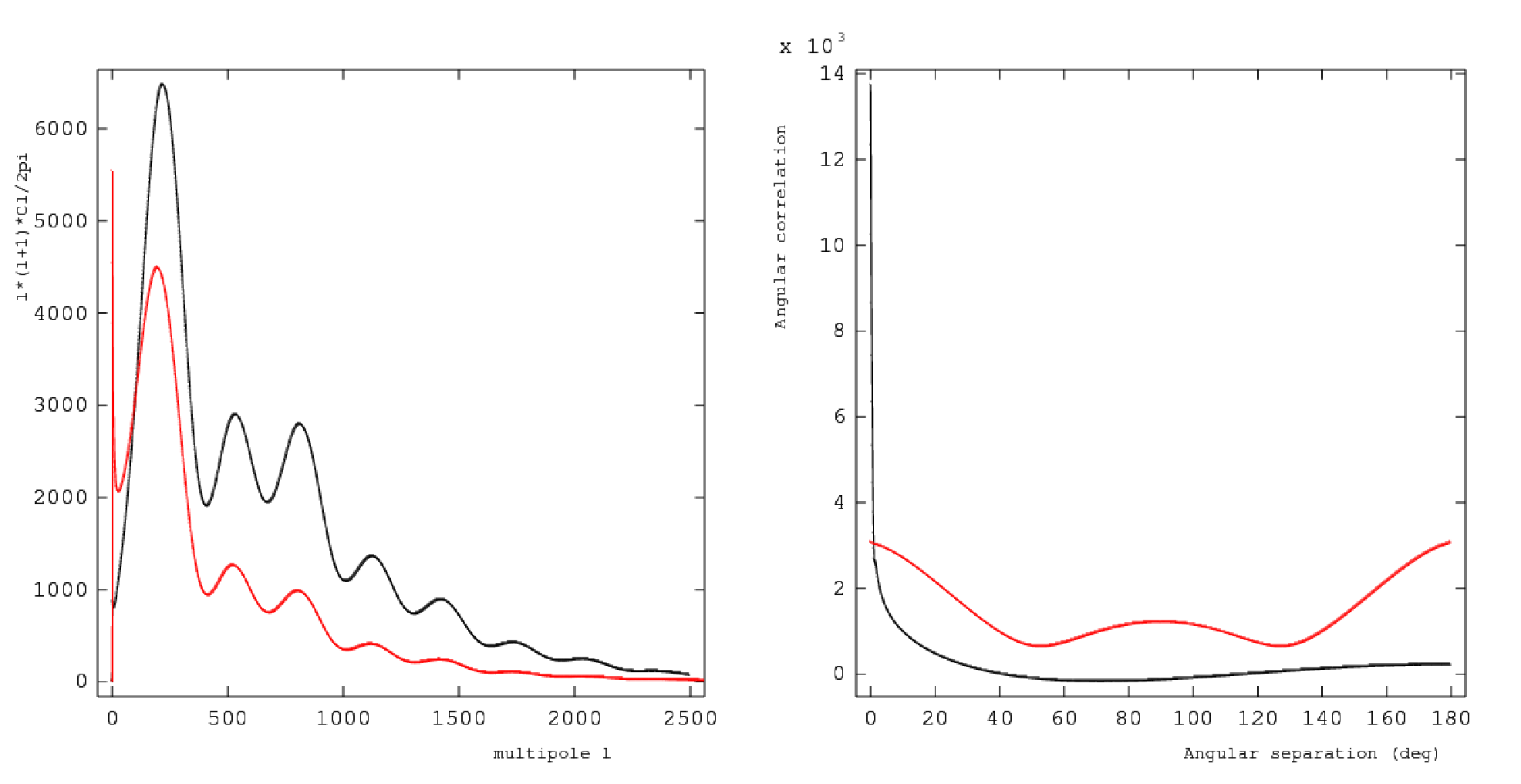
Figure 1 shows an example of a power spectrum $C_{l}$ and the variance of its estimator $\widehat{C}_{l}$ obtain with the CMBFAST code ([Seljak et al, 1996] and [Zaldarriaga et al, 2000]) with the standard set of cosmological parameters.

In order to obtain an estimator $\hat{\xi}$ of the angular correlation function, we can average over all pairs of directions $\;\overrightarrow{\Omega},\overrightarrow{\Omega^{\prime}}\;$ of the observed sky (keeping the angle $\gamma$ between them fixed):

$$\hat{\xi}(\gamma)\;=\;\frac{1}{\mathcal{N}(\gamma)}\;\int\limits_{S^{2}\times S^{2}}\;\overline{T}(\Omega_{1})T(\Omega_{2})\;d\Omega_{1}d\Omega_{2}\;\delta(\overrightarrow{\Omega_{1}}.\overrightarrow{\Omega_{2}}-\cos(\gamma))$$

with

$$\mathcal{N}(\gamma)\;=\;\int\limits_{S^{2}\times S^{2}}\;d\Omega_{1}d\Omega_{2}\;\delta(\overrightarrow{\Omega_{1}}.\overrightarrow{\Omega_{2}}-\cos(\gamma))$$

As $\;T(\Omega)\;=\;\underset{l,m}{\overset{}{\sum}}\;a_{{l}{m}}\;Y_{l}^{m}(\Omega)\;$, we get:

$$\hat{\xi}(\gamma)\;=\;\frac{1}{\mathcal{N}(\gamma)}\underset{l_{1},m_{1}}{\overset{}{\sum}}\underset{l_{2},m_{2}}{\overset{}{\sum}}\;\overline{a_{{l_{1}}{m_{1}}}}\;a_{{l_{2}}{m_{2}}}\;\int\limits_{S^{2}\times S^{2}}\;\overline{Y_{l_{1}}^{m_{1}}}(\Omega_{1})Y_{l_{2}}^{m_{2}}(\Omega_{2})\;d\Omega_{1}d\Omega_{2}\;\delta(\overrightarrow{\Omega_{1}}.\overrightarrow{\Omega_{2}}-\cos(\gamma))$$

The internal integral $\mathcal{I}$ is computed in appendix G and leads to the estimator value:

$$\begin{array}[]{rcl}\hat{\xi}(\gamma)&=&\frac{1}{\mathcal{N}(\gamma)}\underset{l_{1},m_{1}}{\overset{}{\sum}}\underset{l_{2},m_{2}}{\overset{}{\sum}}\;\overline{a_{{l_{1}}{m_{1}}}}\;a_{{l_{2}}{m_{2}}}\;2\pi\;\delta_{l_{1}l_{2}}\;\delta_{m_{1}m_{2}}\;P_{l_{2}}(\cos(\gamma))\\ &=&\frac{1}{\mathcal{N}(\gamma)}\underset{l,m}{\overset{}{\sum}}\;\overline{a_{{l}{m}}}\;a_{{l}{m}}\;2\pi\;P_{l}(\cos(\gamma))\end{array}$$

Averaging over realisations gives us:

$$\begin{array}[]{rcl}<\hat{\xi}(\gamma)>_{ens}&=&\frac{1}{\mathcal{N}(\gamma)}\underset{l,m}{\overset{}{\sum}}\;<\overline{a_{{l}{m}}}\;a_{{l}{m}}>_{ens}\;2\pi\;P_{l}(\cos(\gamma))\\ &=&\frac{1}{\mathcal{N}(\gamma)}\;2\pi\;\underset{l}{\overset{}{\sum}}\;(2l+1)C_{l}\;P_{l}(\cos(\gamma))\end{array}$$

Now $\mathcal{N}(\gamma)$ has to be computed. $\mathcal{N}(\gamma)$ is equal to the previously computed integral with $T(\Omega)=1$. So, replacing $T(\Omega)$ by $\sqrt{4\pi}Y_{0}^{0}(\Omega)$, or $a_{{l}{m}}=\sqrt{4\pi}\delta_{l0}\delta_{m0}$ and $C_{l}=4\pi\delta_{l0}$. As $P_{0}(\cos(\gamma))=1$, one finally obtains $\mathcal{N}(\gamma)\;=\;\mathcal{N}\;=\;8\pi^{2}$ and: {boxitpara}box 0.7

$$<\hat{\xi}(\gamma)>_{ens}\;=\;\xi(\gamma)\;=\;\frac{1}{4\pi}\;\underset{l}{\overset{}{\sum}}\;(2l+1)C_{l}\;P_{l}(\cos(\gamma))$$

(II.8)

The estimator $\hat{\xi}(\gamma)$ is unbiased.

Figure 1 shows the angular correlation function $\xi(\gamma)$ and the variance of its estimator $\hat{\xi}(\gamma)$.

Defining $K=\left(\frac{2\pi}{\mathcal{N}}\right)^{2}$, the covariance of the estimator is:

$$\begin{array}[]{l}\frac{1}{K}\;\left(<\hat{\xi}(\gamma)\hat{\xi}(\gamma^{\prime})>_{ens}\;-\;<\hat{\xi}(\gamma)>_{ens}<\hat{\xi}(\gamma^{\prime})>_{ens}\right)\\ \qquad\qquad\;=\;\underset{lm}{\overset{}{\sum}}\underset{l^{\prime}m^{\prime}}{\overset{}{\sum}}\;P_{l}(\gamma)\;P_{l^{\prime}}(\gamma^{\prime})<a_{{l}{m}}\overline{a_{{l}{m}}}a_{{l^{\prime}}{m^{\prime}}}\overline{a_{{l^{\prime}}{m^{\prime}}}}>_{ens}\\ \qquad\qquad\qquad\qquad\;-\;\underset{lm}{\overset{}{\sum}}\underset{l^{\prime}m^{\prime}}{\overset{}{\sum}}\;P_{l}(\gamma)\;P_{l^{\prime}}(\gamma^{\prime})<a_{{l}{m}}\overline{a_{{l}{m}}}>_{ens}<a_{{l^{\prime}}{m^{\prime}}}\overline{a_{{l^{\prime}}{m^{\prime}}}}>_{ens}\end{array}$$

As the temperature field is real, and provided that the $a_{{l}{m}}$ are gaussian random variables, one has:

$$\begin{array}[]{l}\frac{1}{K}\;\left(<\hat{\xi}(\gamma)\hat{\xi}(\gamma^{\prime})>_{ens}\;-\;<\hat{\xi}(\gamma)>_{ens}<\hat{\xi}(\gamma^{\prime})>_{ens}\right)\\ \quad\;=\;\underset{lm}{\overset{}{\sum}}\underset{l^{\prime}m^{\prime}}{\overset{}{\sum}}\;P_{l}(\gamma)\;P_{l^{\prime}}(\gamma^{\prime})C_{l}C_{l^{\prime}}(1+\delta_{ll^{\prime}}\delta_{mm^{\prime}})\;+\;\underset{lm}{\overset{}{\sum}}\underset{l^{\prime}m^{\prime}}{\overset{}{\sum}}\;P_{l}(\gamma)\;P_{l^{\prime}}(\gamma^{\prime})C_{l}^{2}\delta_{ll^{\prime}}\delta_{m-m^{\prime}}\\ \qquad\qquad\qquad\qquad\;-\;\underset{lm}{\overset{}{\sum}}\underset{l^{\prime}m^{\prime}}{\overset{}{\sum}}\;P_{l}(\gamma)\;P_{l^{\prime}}(\gamma^{\prime})C_{l}C_{l^{\prime}}\\ \quad\;=\;2\;\underset{l}{\overset{}{\sum}}\;C_{l}^{2}\;P_{l}(\gamma)\;P_{l}(\gamma^{\prime})\end{array}$$

Finally, by replacing $K$ by its value, we obtain: {boxitpara}box 0.7

$$<\hat{\xi}(\gamma)\hat{\xi}(\gamma^{\prime})>_{ens}-<\hat{\xi}(\gamma)>_{ens}<\hat{\xi}(\gamma^{\prime})>_{ens}\;=\;\frac{2}{(4\pi)^{2}}\underset{l}{\overset{}{\sum}}(2l+1)C_{l}^{2}\;P_{l}(\gamma)P_{l}(\gamma^{\prime})$$

(II.9)

The estimators of the angular correlation function values

in different directions are correlated.

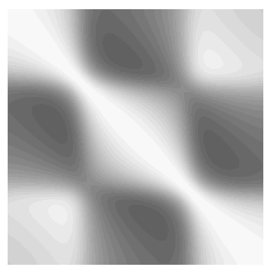
Figure 1 shows the correlation matrix of the angular correlation estimator $\hat{\xi}(\gamma)$.

There are two ways to compute the $C_{l}$ coefficients. Given a temperature field on the sphere, one can compute the $a_{{l}{m}}$ with (II.2) and then the $C_{l}$ using the unbiased estimator (II.6). Equation (II.2) is: $a_{{l}{m}}\sim\int\limits\;P_{l}^{m}(\cos(\theta))d\cos(\theta)\;\int\limits\;T(\theta,\phi)e^{-im\phi}d\phi$.
The inner integral is a Fourier transform which can be fastly computed with the Fast Fourier Transform (FFT) technics (see [Natoli et al, 1997]). Note that this is possible only if the pixels lie on isolatitude lines. The other way is to compute the angular correlation function $\hat{\xi}(\gamma)$, which is unbiased, and then use the second formula in ().

If the observed map is not the full sphere we can adapt these methods. For the first one we can still compute pseudo $a_{{l}{m}}$ by setting the temperature to zero outside the observation zone. This leads to a systematic bias that will be studied in section III. This also introduces correlations among the measured $C_{l}$ and increases their variances. Numerical calculations can be performed in the case where the map is a spherical cap. This is explored in section III and its last section presents detailed comparisons with simulations. This will show that the variance does not depend very much on the map shape. The evolution of the variance with the map size is interpreted in this section.

In section IV we shall discuss the use of the angular correlation function $\hat{\xi}(\gamma)$ measured on the observed map (so the angular separation $\gamma$ is limited to $\gamma_{lim}$). We will show that this quantity is still unbiased, as one intuitively guesses. One can still use the formula () to extract the $C_{l}$ but, since the correlation function is defined only on some interval $[0,\gamma_{lim}]$, the Legendre polynomials are no longer orthogonal. This introduces wild fluctuations in the $C_{l}$. This is cured by ”apodizing” the angular correlation function and will be described in section V.

Four appendices explain technical details to make these notes self contained.

The temperature field is measured on a piece $A$ of the sphere of solid angle $\Omega_{obs}$. We will study the following estimator for the $C_{l}$:

$$\widetilde{C}_{l}\;=\;\frac{1}{2l+1}\;\underset{m=-l}{\overset{l}{\sum}}\mid{\widetilde{a}_{{l}{m}}}\mid^{2}$$

(III.10)

where the $\widetilde{a}_{{l}{m}}$ are computed on $\Omega_{obs}$:

$$\widetilde{a}_{{l}{m}}\;=\;\int\limits_{\Omega_{obs}}T(\Omega)\times\overline{Y_{l}^{m}}(\Omega)\;d\Omega$$

(III.11)

The $\widetilde{C}_{l}$ will therefore represent an estimation of the spectrum of a temperature map which is set to zero outside the observed region. We define the function $W(\overrightarrow{\Omega})$ on the sphere such that $W=1$ on $A$ and $0$ anywhere else.
The temperature field under study is: $T^{\prime}(\Omega)\;=\;(T\times W)(\Omega)$.

The function $W$ can be expanded on spherical harmonics basis as:

	$\displaystyle W(\Omega)$	$\displaystyle=$	$\displaystyle\underset{l=0}{\overset{\infty}{\sum}}\;\underset{m=-l}{\overset{l}{\sum}}b_{{l}{m}}Y_{l}^{m}(\Omega)$		(III.12)
	$\displaystyle b_{{l}{m}}$	$\displaystyle=$	$\displaystyle\int\limits_{S^{2}}\;W(\Omega)\;\overline{Y_{l}^{m}}(\Omega)\;d\Omega\;=\;\int\limits_{\Omega_{obs}}\;\overline{Y_{l}^{m}}(\Omega)\;d\Omega$		(III.13)

Then the $\widetilde{a}_{{l}{m}}$ are:

$$\widetilde{a}_{{l}{m}}\;=\;\int\limits_{S^{2}}T(\Omega)W(\Omega)\;\overline{Y_{l}^{m}(\Omega)}\;d\Omega\;=\;\underset{l^{\prime},m^{\prime},l^{\prime\prime},m^{\prime\prime}}{\overset{}{\sum}}\;a_{{l^{\prime}}{m^{\prime}}}b_{{l^{\prime\prime}}{m^{\prime\prime}}}\int\limits_{S^{2}}Y_{l^{\prime}}^{m^{\prime}}Y_{l^{\prime\prime}}^{m^{\prime\prime}}\overline{Y_{l}^{m}}\;d\Omega$$

Using the property $\;\overline{Y_{l}^{m}}=(-1)^{m}Y_{l}^{-m}$:

$$\widetilde{a}_{{l}{m}}\;=\;\underset{l^{\prime},m^{\prime},l^{\prime\prime},m^{\prime\prime}}{\overset{}{\sum}}\;a_{{l^{\prime}}{m^{\prime}}}b_{{l^{\prime\prime}}{m^{\prime\prime}}}(-1)^{m}\int\limits_{S^{2}}Y_{l^{\prime}}^{m^{\prime}}Y_{l}^{-m}Y_{l^{\prime\prime}}^{m^{\prime\prime}}d\Omega$$

The integral over the sphere of the product of three spherical harmonics is ([Brink et al, 1962] and [Messiah, 1964]):

$$\int\limits_{S^{2}}Y_{a}^{\alpha}Y_{b}^{\beta}Y_{c}^{\gamma}\;\sin(\theta)d\theta d\phi\;=\;\sqrt{\frac{(2a+1)(2b+1)(2c+1)}{4\pi}}\begin{pmatrix}a&b&c\\ \alpha&\beta&\gamma\end{pmatrix}\begin{pmatrix}a&b&c\\ 0&0&0\end{pmatrix}$$

where $\;\begin{pmatrix}a&b&c\\ \alpha&\beta&\gamma\end{pmatrix}\;$ are the Wigner $3j$ symbols related to the Clebsch-Gordan coefficients by:

$$<ab\alpha\beta\mid c-\gamma>\;=\;(-1)^{a-b-\gamma}\sqrt{2c+1}\begin{pmatrix}a&b&c\\ \alpha&\beta&\gamma\end{pmatrix}$$

Recall that these coefficients are real.

$$\begin{array}[]{lcl}\widetilde{a}_{{l}{m}}&=&\underset{l^{\prime},m^{\prime},l^{\prime\prime},m^{\prime\prime}}{\overset{}{\sum}}\;a_{{l^{\prime}}{m^{\prime}}}b_{{l^{\prime\prime}}{m^{\prime\prime}}}(-1)^{m}\sqrt{\frac{(2l+1)(2l^{\prime}+1)(2l^{\prime\prime}+1)}{4\pi}}\begin{pmatrix}l^{\prime}&l&l^{\prime\prime}\\ m^{\prime}&-m&m^{\prime\prime}\end{pmatrix}\begin{pmatrix}l^{\prime}&l&l^{\prime\prime}\\ 0&0&0\end{pmatrix}\\ \overline{\widetilde{a}_{{l}{m}}}&=&\underset{L^{\prime},M^{\prime},L^{\prime\prime},M^{\prime\prime}}{\overset{}{\sum}}\;\overline{a_{{L^{\prime}}{M^{\prime}}}}\overline{b_{{L^{\prime\prime}}{M^{\prime\prime}}}}(-1)^{m}\sqrt{\frac{(2l+1)(2L^{\prime}+1)(2L^{\prime\prime}+1)}{4\pi}}\begin{pmatrix}L^{\prime}&l&L^{\prime\prime}\\ M^{\prime}&-m&M^{\prime\prime}\end{pmatrix}\begin{pmatrix}L^{\prime}&l&L^{\prime\prime}\\ 0&0&0\end{pmatrix}\\ \end{array}$$

	$\displaystyle\mid{\widetilde{a}_{{l}{m}}}\mid^{2}$	$\displaystyle=$	$\displaystyle\widetilde{a}_{{l}{m}}\overline{\widetilde{a}_{{l}{m}}}$
		$\displaystyle=$	$\displaystyle\underset{}{\overset{}{\sum}}\;\;\left(a_{{l^{\prime}}{m^{\prime}}}\overline{a_{{L^{\prime}}{M^{\prime}}}}\right)\left(b_{{l^{\prime\prime}}{m^{\prime\prime}}}\overline{b_{{L^{\prime\prime}}{M^{\prime\prime}}}}\right)\times\frac{2l+1}{4\pi}\sqrt{(2l^{\prime}+1)(2l^{\prime\prime}+1)(2L^{\prime}+1)(2L^{\prime\prime}+1)}$
			$\displaystyle\qquad\qquad\qquad\times\begin{pmatrix}l^{\prime}&l&l^{\prime\prime}\\ m^{\prime}&-m&m^{\prime\prime}\end{pmatrix}\begin{pmatrix}L^{\prime}&l&L^{\prime\prime}\\ M^{\prime}&-m&M^{\prime\prime}\end{pmatrix}\begin{pmatrix}l^{\prime}&l&l^{\prime\prime}\\ 0&0&0\end{pmatrix}\begin{pmatrix}L^{\prime}&l&L^{\prime\prime}\\ 0&0&0\end{pmatrix}$

where the sum runs on $l^{\prime},m^{\prime},l^{\prime\prime},m^{\prime\prime},L^{\prime},M^{\prime},L^{\prime\prime},M^{\prime\prime}$.

The $a_{{l}{m}}$ are random variables. We want to compute the average effect of finite size maps, therefore we shall perform the average over sky realisations (ensemble average²² 2 In the following, we will drop the subscript for ensemble average notations: $\;<\cdots>_{ens}\;\rightarrow\;<\cdots>$ ). Recalling equation (II.3), one obtains:

	$\displaystyle<\widetilde{C}_{l}>$	$\displaystyle=$	$\displaystyle\frac{1}{4\pi}\underset{m=-l}{\overset{l}{\sum}}\;\underset{l^{\prime},m^{\prime},l^{\prime\prime},m^{\prime\prime},L^{\prime\prime},M^{\prime\prime}}{\overset{}{\sum}}C_{l^{\prime}}b_{{l^{\prime\prime}}{m^{\prime\prime}}}\overline{b_{{L^{\prime\prime}}{M^{\prime\prime}}}}(2l^{\prime}+1)\sqrt{(2l^{\prime\prime}+1)(2L^{\prime\prime}+1)}$
			$\displaystyle\qquad\qquad\qquad\times\begin{pmatrix}l^{\prime}&l&l^{\prime\prime}\\ m^{\prime}&-m&m^{\prime\prime}\end{pmatrix}\begin{pmatrix}l^{\prime}&l&L^{\prime\prime}\\ m^{\prime}&-m&M^{\prime\prime}\end{pmatrix}\begin{pmatrix}l^{\prime}&l&l^{\prime\prime}\\ 0&0&0\end{pmatrix}\begin{pmatrix}l^{\prime}&l&L^{\prime\prime}\\ 0&0&0\end{pmatrix}$

Now, remark that the coefficients of the Wigner $3j$ symbol product do not depend on $m$ nor $m^{\prime}$, therefore one can use the orthogonality relations

$$\underset{\alpha\beta}{\overset{}{\sum}}\sqrt{(2c+1)(2c^{\prime}+1)}\begin{pmatrix}a&b&c\\ \alpha&\beta&\gamma\end{pmatrix}\begin{pmatrix}a&b&c^{\prime}\\ \alpha&\beta&\gamma^{\prime}\end{pmatrix}\;=\;\delta_{cc^{\prime}}\delta_{\gamma\gamma^{\prime}}$$

Defining:

$$\mathcal{B}_{l^{\prime\prime}}\;=\;\frac{1}{2l^{\prime\prime}+1}\underset{m^{\prime\prime}=-l^{\prime\prime}}{\overset{l^{\prime\prime}}{\sum}}b_{{l^{\prime\prime}}{m^{\prime\prime}}}\overline{b_{{l^{\prime\prime}}{m^{\prime\prime}}}}$$

(III.14)

we obtain: {boxitpara}box 0.7

$\displaystyle<\widetilde{C}_{l}>$

$\displaystyle=$

$\displaystyle\frac{1}{4\pi}\underset{l^{\prime},l^{\prime\prime}}{\overset{}{\sum}}C_{l^{\prime}}\mathcal{B}_{l^{\prime\prime}}(2l^{\prime}+1)(2l^{\prime\prime}+1)\begin{pmatrix}l^{\prime}&l&l^{\prime\prime}\\ 0&0&0\end{pmatrix}^{2}$

(III.15)

The expression of the $3j$ symbols can be found for instance in [Brink et al, 1962]. We found recently that this calculation has already been published in [Hivon et al, 2002].
The above equation provides the relation between the true $C_{l}$ and the average $<\widetilde{C}_{l}>$ over many sky realisations of the $\widetilde{C}_{l}$ coefficients measured over a patch $A$ of any shape of the sphere. This can be written in matrix form:

$\displaystyle\left[<\widetilde{C}_{l}>\right]\;=\;\left[M\right]_{ll^{\prime}}\times\left[C_{l^{\prime}}\right]\;\mbox{with}\;M_{ll^{\prime}}\;=\;\frac{2l^{\prime}+1}{4\pi}\;\underset{l^{\prime\prime}=0}{\overset{\infty}{\sum}}(2l^{\prime\prime}+1)\mathcal{B}_{l^{\prime\prime}}\begin{pmatrix}l^{\prime}&l&l^{\prime\prime}\\ 0&0&0\end{pmatrix}^{2}$

(III.16)

This result is valid for any weighting function $W$ on the sphere. The relation between the $\widetilde{C}_{l}$ and the $C_{l}$ is linear. The matrix $M_{ll^{\prime}}$ depends only on the map shape and not on the initial $C_{l^{\prime}}$ spectrum. Permutations of $2$ columns of the $3j$ symbols change their values by a phase ([Messiah, 1964]) so $\;(2l+1)M_{ll^{\prime}}=(2l^{\prime}+1)M_{l^{\prime}l}$. The $M_{ll^{\prime}}$ elements are positive or null.

When the full sky is observed, $\;\mathcal{B}_{l^{\prime\prime}}=\mathcal{B}_{0}\delta_{l^{\prime\prime}0}\;$ and the $3j$ symbols imply $l=l^{\prime}$ whence $M_{ll^{\prime}}$ is the identity matrix.
On the other hand, when observing a portion of the sky, each measured $\widetilde{C}_{l}$ is a mixture of the $C_{l}$ whose weights are given by the matrix $M_{ll^{\prime}}$.

The properties of the matrix are illustrated in figure 4. The bottom graphs show line $l=1500$ of matrix $M_{ll^{\prime}}$ for a $10\times 10\;deg^{2}$ map and lines $l=500,2400$ where the peaks have been shifted to $l^{\prime}=1500$ for easy comparison: the width of the peak is nearly constant with $l$, that is to say that the matrix is nearly band-diagonal.
The top graphs show the $M_{ll^{\prime}}$ element values of line $l=1500$ for maps of various size and shapes. As the map size decreases, the peak width gets larger and a given $\widetilde{C}_{l}$ measurement involves a larger band in $C_{l^{\prime}}$. The width of the peak is inversely proportionnal to the caracteristic width of the map and it does not depend very much on the shape provided it is not excessively elongated. This is somewhat equivalent to what we have in Fourier analysis on small intervals.
The $C_{l}$ are coefficients in the correlation function expansion (). The $P_{l}$ are orthogonal on $[0,\pi]$ and form a basis on this interval. On a partial map of characteristic size $\theta_{c}$ these functions are ”nearly orthogonal” if they differ by more than $\delta l\simeq\pi/\theta_{c}$: loosely speaking if they have not the same number of roots in that interval. Therefore, for a given correlation function, the $\widetilde{C}_{l}$ will be mixtures of the ”true” $C_{l}$ over a range $\simeq\delta l$.

If $\Omega_{obs}$ is the solid angle corresponding to the observed patch of the sky, using the completude relation for the spherical harmonics, we have for the $\mathcal{B}_{l}$ normalisation:

$\displaystyle\underset{l=0}{\overset{\infty}{\sum}}(2l+1)\mathcal{B}_{l}\;=\;\underset{l=0}{\overset{\infty}{\sum}}\;\underset{m=-l}{\overset{l}{\sum}}b_{{l}{m}}\overline{b_{{l}{m}}}\;=\;\int\limits_{S^{2}}\;\mid{W(\overrightarrow{\Omega})}\mid^{2}\;d\overrightarrow{\Omega}$

Until the end of this section, we assume that $W=1$ on $A$ and zero elsewhere. Thus we have:

$\displaystyle\underset{l=0}{\overset{\infty}{\sum}}(2l+1)\mathcal{B}_{l}\;=\;\Omega_{obs}$

(III.17)

The $\widetilde{C}_{l}$ are biased relative to the $C_{l}$ since one observes only a fraction of the sphere, the rest being $0$. Assuming that the function $T$ is isotropic, to compare the $\widetilde{C}_{l}$ with $C_{l}$ one has to take into account the sky coverage normalisation:

$$<\widetilde{C}_{l}^{R}>\;=\;\frac{4\pi}{\Omega_{obs}}\times<\widetilde{C}_{l}>\;=\;\underset{l^{\prime}}{\overset{}{\sum}}\;M_{ll^{\prime}}^{R}\times C_{l^{\prime}}\quad\mbox{where}\quad M_{ll^{\prime}}^{R}\;=\;\frac{4\pi}{\Omega_{obs}}M_{ll^{\prime}}$$

(III.18)

In the following, when talking about comparison between $\widetilde{C}_{l}$ and $C_{l}$, we will assume that the $\widetilde{C}_{l}$ have been renormalised as describe above.

Using the $3j$ orthogonality relation ([Messiah, 1964], appendix C relation $15b$) which gives $\quad\underset{l^{\prime}}{\overset{}{\sum}}(2l^{\prime}+1)\begin{pmatrix}l^{\prime}&l&l^{\prime\prime}\\ 0&0&0\end{pmatrix}^{2}=1\quad$ and equation (III.17) we get $\;\;\underset{l^{\prime}}{\overset{}{\sum}}\;M_{ll^{\prime}}^{R}=1$.
Therefore for a given $<\widetilde{C}_{l}^{R}>$, the sum of the weights of the $C_{l^{\prime}}$ is equal to one.

The $\mathcal{B}_{l}$ can be obtain using usual computer technics (see [Gòrski et al, 2005]). Then it is easy and fast to compute numerically the matrix $M_{ll^{\prime}}$ and check the systematic effect of finite size map.
The figure 2 shows the $\mathcal{B}_{l}$ spectrum and the $M_{ll^{\prime}}$ matrice for a $10\times 10\;deg^{2}$ square map.

We have tried to compute the variance of the $\widetilde{C}_{l}$ estimator following the same line of calculation. Although the result does not look like too complicated, it is of little use, because it would cost a lot of computer time to be numerically calculated in the general case. However it can be calculated in the simple case of a spherical cap domain.

If, in equation (III.11), we replace the temperature field by its expression (II.1), we get:

$$\widetilde{a}_{{l}{m}}\;=\;\underset{l_{1}m_{1}}{\overset{}{\sum}}\;a_{{l_{1}}{m_{1}}}\;B_{l_{1}m_{1}lm}$$

where we have set:

$$B_{l_{1}m_{1}lm}\;=\;\int\limits_{S^{2}}\;W(\overrightarrow{\Omega})\;Y_{l_{1}}^{m_{1}}(\overrightarrow{\Omega})\;\overline{Y_{l}^{m}}(\overrightarrow{\Omega})\;d\overrightarrow{\Omega}$$

Averaging over sky realisations and using equation (II.3), one gets (see details in appendix H):

$$<\widetilde{C}_{l}>\;=\;\frac{1}{2l+1}\;\underset{ml^{\prime}m^{\prime}}{\overset{}{\sum}}C_{l^{\prime}}\mid{B_{lml^{\prime}m^{\prime}}}\mid^{2}\qquad\mbox{for}\quad-l\leq m\leq+l\;,\;0\leq l^{\prime}<\infty\;,\;-l^{\prime}\leq m^{\prime}\leq+l^{\prime}$$

and provided that the $a_{{l}{m}}$ are gaussian random fields:

$$<\widetilde{C}_{l}\widetilde{C}_{L}>-<\widetilde{C}_{l}><\widetilde{C}_{L}>\;=\;\frac{2}{(2l+1)(2L+1)}\underset{m=-l}{\overset{+l}{\sum}}\;\underset{M=-L}{\overset{+L}{\sum}}\mid{\underset{l^{\prime}}{\overset{}{\sum}}C_{l^{\prime}}\underset{m^{\prime}=-l^{\prime}}{\overset{+l^{\prime}}{\sum}}B_{l^{\prime}m^{\prime}lm}\overline{B_{l^{\prime}m^{\prime}LM}}}\mid^{2}$$

The last two results are valid for any weighting function $W$ on the sphere. $W$ could include an additionnal weighting, for instance to treat border effects. The results of the former section can also be adapted to that case. Until the end of this section, we will assume that $W=1$ on $A$ and zero elsewhere.

This equation simplifies a lot if one considers a spherical cap centered at the north pole with border at polar angle $\theta_{c}$. Using $Y_{l}^{m}(\theta,\phi)\;=\;\lambda_{l}^{m}(\cos(\theta))\;e^{im\phi}\;$ (where $\lambda_{l}^{m}$ are the normalised associated Legendre polynomials), we get in this case:

$B_{lmLM}\;=\;2\pi\;\delta_{mM}\;B_{lLm}\qquad$ where³³ 3 We have $\;B_{ll^{\prime}m}\;=\;B_{l^{\prime}lm}\;=\;B_{ll^{\prime}-m}\in\mathbb{R}\;$, $\;B_{000}\;=\;\frac{1}{4\pi}\;(1-\cos(\theta_{c}))\;$, $B_{ll^{\prime}m}=0$ for $\mid{m}\mid>\min(l,l^{\prime})$.
From the relation $\;\underset{m}{\overset{}{\sum}}\overline{Y_{l}^{m}}(\overrightarrow{\Omega_{1}})Y_{l}^{m}(\overrightarrow{\Omega_{2}})=\frac{2l+1}{4\pi}P_{l}(\overrightarrow{\Omega_{1}}.\overrightarrow{\Omega_{2}})\;$ we get $\;\underset{m}{\overset{}{\sum}}\;B_{llm}\;=\;\frac{2l+1}{8\pi^{2}}\;\Omega_{obs}$ $\qquad B_{lLm}\;=\;\;\int\limits_{0}^{\theta_{c}}\;\lambda_{l}^{m}(\cos(\theta))\;\lambda_{L}^{m}(\cos(\theta))\;d\cos(\theta)$

Replacing in the general expression for the covariance, one obtains:

$\displaystyle<\widetilde{C}_{l}>\;=\;\frac{(2\pi)^{2}}{2l+1}\;\underset{m=-l}{\overset{l}{\sum}}\;\;\underset{l^{\prime}\geq\mid{m}\mid}{\overset{}{\sum}}\;C_{l^{\prime}}\;(B_{ll^{\prime}m})^{2}$

(III.19)

and for the covariance:

$$<\widetilde{C}_{l}\widetilde{C}_{L}>-<\widetilde{C}_{l}><\widetilde{C}_{L}>\;=\;\frac{2\;(2\pi)^{4}}{(2l+1)(2L+1)}\;\underset{m}{\overset{}{\sum}}\;\left(\underset{l^{\prime}\geq\mid{m}\mid}{\overset{}{\sum}}\;C_{l^{\prime}}\;B_{ll^{\prime}m}B_{Ll^{\prime}m}\;\right)^{2}$$

(III.20)

The $B_{ll^{\prime}m}$ coefficients could be computed by numerical integration but this would be very slow at high $l$. The calculations were done using recurrence relations.
The figure 3 shows the correlation matrix computed from the covariance formula above for a $10\times 10\;deg^{2}$ spherical cap.

Recurrence relations
In order to derive the following recurrence relations for the $B_{ll^{\prime}m}$ coefficients, we have used the usual recurrence relations among the normalised associated Legendre functions ([Gradshtein et al, 1980]) which imply integrals of the form⁴⁴ 4 We set $\;c=\cos(\theta_{c})\;$ and $\;x=\cos(\theta)$ $\;\int\limits_{1}^{c}x\lambda_{l}^{m}(x)\lambda_{k}^{m}(x)dx$. The latter integration can be in turn related to integrals of the type $\;\int\limits_{1}^{c}\lambda_{l}^{m}(x)\lambda_{k}^{m}(x)dx\;$ by evaluating $\;\int\limits_{1}^{c}(1-x^{2})(\lambda_{l}^{m}{{}^{\prime}}\lambda_{k}^{m}{{}^{\prime\prime}}+\lambda_{l}^{m}{{}^{\prime\prime}}\lambda_{k}^{m}{{}^{\prime}})dx\;$ and using the Legendre differential equation (where ^′ and ^′′ means first and second order derivations with respect to $x$). One gets:

$$\begin{array}[]{rcl}B_{l,l+1,m}&=&-c\lambda_{l}^{m}(c)\lambda_{l+1}^{m}(c)\;+\;\frac{\sqrt{(l+1-m)(l+1+m)}}{2(l+1)}\left(\sqrt{\frac{2l+3}{2l+1}}\;[\lambda_{l}^{m}(c)]^{2}\;+\;\sqrt{\frac{2l+1}{2l+3}}\;[\lambda_{l+1}^{m}(c)]^{2}\right)\end{array}$$

And for $\;\mid{k-l}\mid\geq 2$, setting $\;b=(l+1)(k-l)(k-m)$, one has:

	$\displaystyle b\times B_{lkm}$	$\displaystyle=$	$\displaystyle k\sqrt{\frac{2k+1}{2k-1}}\sqrt{\frac{2l+1}{2l+3}}\sqrt{\frac{k-m}{k+m}}\sqrt{\frac{l+1-m}{l+1+m}}(k-l-2)(l+1+m)\;B_{l+1,k-1,m}$		(III.21)
			$\displaystyle-\;(k-m)\left((l+1)c\lambda_{l}^{m}(c)-\sqrt{\frac{2l+1}{2l+3}}\sqrt{\frac{l+1+m}{l+1-m}}(l+1-m)\lambda_{l+1}^{m}(c)\right)\lambda_{k}^{m}(c)$
			$\displaystyle-\;\sqrt{\frac{2k+1}{2k-1}}\sqrt{\frac{k-m}{k+m}}\;\lambda_{k-1}^{m}(c)$
			$\displaystyle\qquad\times\left(k\sqrt{\frac{2l+1}{2l+3}}\sqrt{\frac{l+1-m}{l+1+m}}(l+1+m)c\lambda_{l+1}^{m}(c)-(k(l+1)-m^{2})\lambda_{l}^{m}(c)\right)$

This heavy recurrence relation has been verified to be numerically stable up to $l\simeq 2500$.
The only numerical integral to perform is $\;B_{llm}$. As $\lambda_{l}^{m}(x)\;\sim\;(1-x^{2})^{\frac{1}{2}m}\;Q(l-m)$ (where $Q(n)$ stands for a polynome of degree $n$), the integrand of $B_{llm}$ is a polynome of degree $2l$ and it may be exactly computed using the Gauss-Legendre integration method with $l+1$ points. All other $B_{lkm}$ can be computed using the recurrence relations (III.21).
With similar technics [Wandelt et al, 2001] derived different equivalent recurrence relations.

Approximation for small maps
For small $\theta_{c}$ ($\theta_{c}\lesssim 0.15$), one can make the approximation ([Gradshtein et al, 1980]):

$$\lambda_{l}^{m}\left(\cos(\theta)\right)\;\rightarrow\;\frac{(-1)^{m}}{l^{m}}\;\sqrt{\frac{(2l+1)(l+m)!}{4\pi(l-m)!}}\;J_{m}(l\theta)$$

where the $J_{m}$ are the cylindrical Bessel functions. Therefore:

$$B_{l_{1}lm}\;\simeq\;\sqrt{\frac{2l+1}{4\pi}\;\frac{2l_{1}+1}{4\pi}\;\frac{(l+m)!}{(l-m)!}\frac{(l_{1}+m)!}{(l_{1}-m)!}}\;\;\frac{1}{l_{1}^{m}l^{m}}\;\;\int\limits_{0}^{\theta_{c}}\theta\;J_{m}(l_{1}\theta)\;J_{m}(l\theta)\;d\theta$$

where the last integral is a Lommel integral ([Gradshtein et al, 1980]). Then:

	$\displaystyle B_{l_{1}lm}\simeq\sqrt{\frac{2l+1}{4\pi}\;\frac{2l_{1}+1}{4\pi}\;\frac{(l+m)!}{(l-m)!}\frac{(l_{1}+m)!}{(l_{1}-m)!}}\;\;\frac{1}{l_{1}^{m}l^{m}}\;\;\frac{\theta_{c}}{l_{1}^{2}-l^{2}}$
	$\displaystyle\qquad\qquad\times\left\{lJ_{m}(l_{1}\theta_{c})J^{\prime}_{m}(l\theta_{c})-l_{1}J_{m}(l\theta_{c})J^{\prime}_{m}(l_{1}\theta_{c})\right\}\$		(III.22)

where $J^{\prime}_{m}(z)$ stands for the derivative of $J_{m}(z)$ relative to $z$.
For numerical purposes it is easier to replace $\left\{lJ_{m}(l_{1}\theta_{c})J^{\prime}_{m}(l\theta_{c})-l_{1}J_{m}(l\theta_{c})J^{\prime}_{m}(l_{1}\theta_{c})\right\}$ by $\left\{l_{1}J_{m}(l\theta_{c})J_{m+1}(l_{1}\theta_{c})-lJ_{m}(l_{1}\theta_{c})J_{m+1}(l\theta_{c})\right\}$. Figure 9 compares the variance of the $\widetilde{C}_{l}^{R}$ computed with relation (III.21) with the calculation done with the above approximation: the agreement is excellent for $f_{sky}\;=\;\frac{\Omega_{obs}}{4\pi}\lesssim 6\;10^{-3}\;\;$ ($\theta_{c}\lesssim 0.15\;rd$).

Behaviour of the variance as a function of $\theta_{c}$
If $l\theta_{c}<m$, $\;J_{m}(l\theta_{c})$ behaves as $(l\theta_{c})^{m}$ which gives a negligible contribution if $m$ is large. On the other hand, if $m<l\theta_{c}$ one can use the following approximation ([Gradshtein et al, 1980]):

$$J_{m}(l\theta_{c})\;\simeq\;\;\sqrt{\frac{2}{\pi}}\;\frac{1}{\sqrt{l\theta_{c}}}\;\cos(l\theta_{c}+\phi_{m})$$

where $\phi_{m}$ is a phase depending on $m$ and slowly varying with $l\theta_{c}$: $\;\phi_{m}\rightarrow-m\frac{\pi}{2}-\frac{\pi}{4}\;\;$ for $\;\;l\theta_{c}\rightarrow\infty$.
In that approximation, from equation (III.22) one obtains⁵⁵ 5 This equation and (III.19) explain qualitatively the behaviour of the matrix $M_{ll^{\prime}}$. :

$$B_{l_{1}lm}\;\sim\;\frac{\sin((l_{1}-l)\theta^{\prime}_{c})}{l_{1}-l}\qquad\theta^{\prime}_{c}=\theta_{c}\;+\;\mbox{corrections depending on}\;m$$

(III.23)

One can use this approximation in equation (III.20) in which we set $l=L$ for the variance calculation.

References

• [Benoit et al, 2003] Benoit,A. et al (The Archeops Collaboration), A&A,399, p.L19-L23 (2003)
• [Brink et al, 1962] Brink,D.M.; Satchler,G.R., Angular Momentum (Clarendon Press 1962)
• [De Bernardis et al, 2000] De Bernardis, P., Ade, P. A. R., Bock, J. J., et al. 2000, Nature, 404, 955
• [Gòrski et al, 2005] Gòrski, K. M., Hivon, E., Banday, A. J., et al. 2005, ApJ , 622, 759 (see also http://healpix.jpl.nasa.gov)
• [Gradshtein et al, 1980] Gradshtein I.S.; Ryzhik,I.M.; Jeffrey,A., Table of integrals, series, and products (Academic Press 1980)
• [Hanany et al, 2000] Hanany, S., Ade, P., Balbi, A., et al. 2000, ApJ , 545, L5
• [Hivon et al, 2002] Hivon et al, The Astrophysical Journal, Volume 567, Issue 1, pp. 2-17 (2002).
• [Masi et al, 2006] S.Masi, et al. 17th ESA Symposium on European Rocket and Balloon Programmes and Related Research, 30 May-2 June 2005, Sandefjord, Norway. ESA Publications Division, ISBN 92-9092-901-4, 2005, p 581-586.
• [Messiah, 1964] Messiah,A. mécanique quantique Tome 2 (Editions DUNOD, paris 1964)
• [Natoli et al, 1997] P. Natoli, P.F. Muciaccia, and N. Vittorio, ApJ Letter 488, L63 (1997).
• [Seljak et al, 1996] Seljak, U., Zaldarriaga, M., 1996 ApJ, 469, 437 (see also http://www.cmbfast.org)
• [Tegmark, 1997] Tegmark, M. 1997, PrD , 56, 4514
• [Wandelt et al, 2001] Wandelt et al, Physical Review D (Particles, Fields, Gravitation, and Cosmology), Volume 64, Issue 8, 15 October 2001
• [Zaldarriaga et al, 2000] Zaldarriaga, M., Seljak, U., 2000 ApJS, 129, pp 431-434