Determination of light quark masses from the electromagnetic splitting of pseudoscalar meson masses computed with two flavors of domain wall fermions

Here we identify the global symmetry of the continuum QCD+QED system and the related Ward-Takahashi identity. For now we set all quark masses to zero.

In pure QCD, the global symmetry of the fermion action is $G_{\rm QCD}=SU(3)_{L}\times SU(3)_{R}\times U(1)_{V}$, where $U(1)_{V}$ represents the baryon number charge and $SU(3)_{L,R}$ are independent flavor rotations on the left and right handed light quark fields, respectively. $U(1)_{A}$ does not exist due to the axial anomaly. The symmetry which survives after spontaneous chiral symmetry breaking due to QCD dynamics is the vectorial part of $G_{\rm QCD}$, i.e., $H_{\rm QCD}=SU(3)_{V}\times U(1)_{V}$.

The QCD+QED system is obtained by introducing the EM interaction of quarks $q=(u,\,d,\,s)^{T}$ with the $U(1)_{\rm em}$ gauge potential $A_{{\rm em}\,\mu}$ as

	$\displaystyle S_{\rm em}$	$\displaystyle=$	$\displaystyle\int d^{4}x\,ej_{\rm em}^{\mu}\,A_{{\rm em}\,\mu}\,,$		(1)
	$\displaystyle j_{\rm em}^{\mu}$	$\displaystyle=$	$\displaystyle\overline{q}\gamma^{\mu}Q_{\rm em}q\,,$		(2)

where $j_{\rm em}^{\mu}$ is the electromagnetic current, and $Q_{\rm em}$ is the $3\times 3$ matrix of the electric charges of the quarks.

$\displaystyle Q_{\rm em}=\left(\begin{array}[]{ccc}\frac{2}{3}&0&0\\ 0&-\frac{1}{3}&0\\ 0&0&-\frac{1}{3}\end{array}\right)\,.$

It is convenient to express $Q_{\rm em}$ in terms of the generators $\left\{T^{a}\right\}_{a=1,\,\cdots,\,8}$ of $SU(3)$, which can be given by $T^{a}=\frac{\lambda^{a}}{2}$ with $\lambda^{a}$ the Gell-Mann matrices and satisfy ${\rm tr}\left(T^{a}T^{b}\right)=\frac{1}{2}\delta^{ab}$, as

$\displaystyle Q_{\rm em}=T^{3}+\frac{1}{\sqrt{3}}T^{8}\,.$

(7)

The EM interaction $S_{\rm em}$ breaks a part of $G_{\rm QCD}$. This can be seen explicitly by looking at the modified Ward-Takahashi identity for the flavor-nonsinglet axial-vector current, $A^{a}_{\mu}\equiv\overline{q}\gamma_{\mu}\gamma_{5}T^{a}q$,

$\displaystyle\partial^{\mu}A^{a}_{\mu}=ieA_{{\rm em}\,\mu}\,\overline{q}\left[T^{a},\,Q_{\rm em}\right]\gamma^{\mu}\gamma_{5}q-\frac{\alpha}{2\pi}\,{\rm tr}\left(Q_{\rm em}^{2}T^{a}\right)F_{\rm em}^{\mu\nu}\widetilde{F}_{{\rm em}\,\mu\nu}\,,$

(8)

where $F_{{\rm em}\,\mu\nu}=\partial_{\mu}A_{{\rm em}\,\nu}-\partial_{\nu}A_{{\rm em}\,\mu}$ is the field strength of the electromagnetic field, $\widetilde{F}_{{\rm em}\,\mu\nu}\equiv\frac{1}{2}\varepsilon_{\mu\nu\lambda\rho}F_{\rm em}^{\lambda\rho}$, and we still have the light quark masses set to zero. The second term on the right hand side arises from the QED chiral anomaly. The first term on the right hand side vanishes for $a=3,\,6,\,7,\,8$ in the Gell-Mann basis while the second term does so for $a=1,\,2,\,4,\,5,\,6,\,7$, and a linear combination of $a=$ 3 and 8,

$\displaystyle\frac{1}{2}T^{\prime\,3}$

$\displaystyle\equiv$

$\displaystyle\frac{\sqrt{3}}{2}T^{8}-\frac{1}{2}T^{3}=\frac{1}{2}\left(\begin{array}[]{ccc}0&0&0\\ 0&1&0\\ 0&0&-1\end{array}\right)\,.$

Thus the global symmetry present in this system is

$\displaystyle G_{\rm QCD+QED}=SU(2)^{\prime}_{L}\times SU(2)^{\prime}_{R}\times U(1)_{\rm em}\times U(1)_{V}\,,$

(13)

where $SU(2)^{\prime}_{L,\,R}$ are the subgroups of $SU(3)_{L,\,R}$ generated by $T^{6},\,T^{7},\,T^{\prime\,3}$. QCD dynamics breaks $G_{\rm QCD+QED}$ spontaneously down to the vector-like symmetry

$\displaystyle H_{\rm QCD+QED}=SU(2)^{\prime}_{V}\times U(1)_{\rm em}\times U(1)_{V}\,.$

(14)

The exact Nambu-Goldstone (NG) bosons associated with this spontaneous symmetry breaking in massless QCD+QED are $K^{0}$, $\overline{K}^{0}$ and a neutral meson corresponding to the generator $T^{\,\prime\,3}$, i.e., $d\bar{d}-s\bar{s}$.

Now remember that without the second term on the right hand side of Eq. (8) due to the QED anomaly, four neutral mesons are massless in the chiral limit as Eq. (8) then vanishes for $a=$3, 6, 7, and 8. In other words, the QED anomaly may make the meson corresponding to the generator $Q_{\rm em}$ massive. This meson acquires its mass through a diagram consisting of two quark triangles connected by two photons, which is ${\cal O}(\alpha^{2})$. Since we neglect ${\cal O}(\alpha^{2})$-effects throughout this work, we will consider this meson as a NG boson up to this approximation. Neglecting the QED anomaly term, the pattern of chiral symmetry breaking in massless QCD+QED reads

	$\displaystyle\widehat{G}_{\rm QCD+QED}=SU(2)^{\prime}_{L}\times U(1)^{\prime\prime}_{L}\times SU(2)^{\prime}_{R}\times U(1)^{\prime\prime}_{R}\times U(1)_{V}$
	$\displaystyle\quad\Rightarrow\widehat{H}_{\rm QCD+QED}=SU(2)^{\prime}_{V}\times U(1)_{\rm em}\times U(1)_{V}\,.$		(15)

Here $U(1)^{\prime\prime}_{L/R}$ are the subgroups of $SU(3)_{L/R}$ generated by $Q_{\rm em}$, respectively. The Goldstone bosons associated with this pattern are the strange mesons $K^{0}$, $\bar{K}^{0}$ and $\pi_{3}$, $\eta_{8}$ corresponding to $T^{3}$, $T^{8}$.

In pure QCD, as long as $m_{u}=m_{d}$, isospin symmetry remains unbroken, and we need consider only the connected (quark) diagram in the neutral pion correlation function since the disconnected ones cancel exactly²² 2 The interpolating operator for $\pi_{3}$ is $(\bar{u}\gamma_{5}u-\bar{d}\gamma_{5}d)/\sqrt{2}$, so in pure QCD the four resulting disconnected diagrams in the correlation function $\langle\pi_{3}\pi_{3}\rangle$ cancel. Once isospin symmetry is broken, the up and down quark loops are no longer equal and hence do not cancel.. However, once the EM interaction and the $u$-$d$ mass difference are introduced, disconnected diagrams no longer cancel and must be included. Then two complications arise; one is the mixing of neutral pseudoscalar mesons and the other is the appearance of the two-photon state as the ground state³³ 3 Since the two-photon state must carry orbital angular momentum, each photon has non-zero momentum. With our lattice setup, the possible minimum energy for this state is about 1.3 GeV. Therefore we could have neglected this state even if we had included disconnected diagrams since the possible minimum energy is much larger than the NG boson masses. . Due to the well known computational difficulty associated with disconnected diagrams, we neglect their contributions everywhere in our current study. Thus we need to know how this approximation affects the pion mass. Remember that calculating the connected diagram only is equivalent to calculating the mass of the neutral kaon, and the neutral kaon is massless in the chiral limit in the presence of the EM interaction as discussed in Sec. II.1. Therefore the neutral pion mass computed with only connected diagrams does not have a term of $O(\alpha)$ in the chiral limit.

For clarity, let $\pi_{3}$ and $\pi^{0}$ denote the neutral pion in the basis of flavor eigenstates and mass eigenstates, respectively. In Sec. II.1, we discussed that including terms of $O(\alpha)$, the neutral pion corresponding to $T^{3}$, i.e. ${\pi_{3}}$, is massless when $m_{u}=m_{d}=0$. In general, the mass of the physical neutral pion, $m_{\pi^{0}}$, is different from $m_{\pi_{3}}$ due to the mixing with other neutral pseudoscalar mesons. Following the classic current algebra treatment of $\pi_{3}-\eta$ mixing Gross:1979ur and the $\pi_{3}-\eta^{\prime}$ mixing Gasser:1984gg based on ChPT or a version of that, in pure QCD with $m_{u}\neq m_{d}$ the contribution to $m_{\pi^{0}}^{2}$ is estimated to be proportional to $(m_{u}-m_{d})^{2}/m_{s}^{2}$. Repeating a similar treatment for the EM interaction, it turns out that the fact that $m_{\pi^{0}}^{2}$, including $O(\alpha)$ corrections, vanishes in the chiral limit does not change. Hence, the mass-squared of $\pi^{0}$ begins at second order in the isospin breaking $(m_{u}-m_{d})^{2}$ and/or $\alpha^{2}$. Since we neglect effects of this order throughout this work, we can identify “the neutral pion” consisting of only connected diagrams with that of $\pi^{0}$.

In summary, as long as we discuss the squared pseudoscalar meson mass and neglect ${\cal O}(\alpha^{2})$ and ${\cal O}((m_{u}-m_{d})^{2})$-effects, “the neutral pion mass” in this work is approximately equal to the physical $\pi^{0}$ mass, and the difference can arise at ${\cal O}(\alpha m)$.

We consider the QCD+QED system on the lattice with two flavors of domain wall quarks, $q_{1}$ and $q_{2}$, which have mass $m_{\rm val,1}$ and $m_{\rm val,2}$ and charge $Q_{\rm val,1}$ and $Q_{\rm val,2}$, respectively. These fields are valence quark fields. The flavor non-singlet axial Ward-Takahashi (WT) identity associated with the chiral transformation of the valence quark fields is given by

	$\displaystyle\partial_{\mu}^{*}{\cal A}^{a}_{\mu}(x)$	$\displaystyle=$	$\displaystyle(m_{\rm val,1}+m_{\rm val,2})\,P^{a}(x)+(m_{\rm val,1}-m_{\rm val,2})\,\bar{q}(x)\gamma_{5}\left\{\frac{\tau^{a}}{2},\frac{\tau^{3}}{2}\right\}\,q(x)$		(16)
			$\displaystyle\ +2\,J_{5q}^{a}(x)+\sum_{s}\epsilon(s){\cal X}_{s}^{a}(x)\,,$

where $q=\left(q_{1},q_{2}\right)^{T}$, ${\cal A}_{\mu}^{a}(x)$ is the conserved axial-vector current whose form is the same as that in the pure QCD domain wall fermion system Furman:1994ky, but the link variables are now replaced with

$\displaystyle\left(\begin{array}[]{cc}U_{{\rm QCD},\,\mu}(x)\left(U_{{\rm em},\,\mu}(x)\right)^{eQ_{\rm val,1}}&0\\ 0&U_{\rm QCD,\,\it\mu}(x)\left(U_{{\rm em},\,\mu}(x)\right)^{eQ_{\rm val,2}}\end{array}\right)\,.$

$P^{a}(x)$ and $J_{5q}^{a}(x)$ denote pseudoscalar densities. While $P^{a}(x)$ contains physical quark fields only, $J_{5q}^{a}(x)$ is defined at the midpoint of the fifth dimension and written in terms of bulk fields, as in the pure QCD case Furman:1994ky. ${\cal X}_{s}^{a}(x)$ is give by

	$\displaystyle{\cal X}_{s}^{a}(x)$	$\displaystyle=$	$\displaystyle-\frac{1}{2}\sum_{\mu}\left[\bar{\Psi}_{s}(x)(1-\gamma_{\mu})U_{{\rm QCD},\,\mu}(x)\right.$		(20)
			$\displaystyle\qquad\qquad\times\left((U_{\rm em,\it\mu}(x))^{eQ_{\rm val,1}}-(U_{\rm em,\it\mu}(x))^{eQ_{\rm val,2}}\right)\left[\frac{\tau^{a}}{2},\frac{\tau^{3}}{2}\right]\Psi_{s}(x+\widehat{\mu})$
			$\displaystyle\qquad\quad+\bar{\Psi}_{s}(x)(1+\gamma_{\mu})U^{\dagger}_{{\rm QCD}\,\,\mu}(x-\widehat{\mu})\,$
			$\displaystyle\qquad\qquad\times\left(\left(U^{\dagger}_{{\rm em}\,\,\mu}(x-\widehat{\mu})\right)^{eQ_{\rm val,1}}-\left(U^{\dagger}_{{\rm em},\,\mu}(x-\widehat{\mu})\right)^{eQ_{\rm val,2}}\right)$
			$\displaystyle\qquad\qquad\left.\times\left[\frac{\tau^{a}}{2},\frac{\tau^{3}}{2}\right]\Psi_{s}(x-\widehat{\mu})\right],$

where the lattice spacing is set to $1$, $\epsilon(s)=1$ for $0\leq s\leq L_{s}/2-1$ and $-1$ for $L_{s}/2\leq s<L_{s}$. ${\cal X}_{s}^{a}(x)$ vanishes when $a=3$, $e=0$ or $Q_{\rm val,1}=Q_{\rm val,2}$, so it is the lattice counterpart to the first term in Eq. (8). The formula analogous to Eq. (16) is written down for three flavor case. From the analogy to the pure QCD case in the domain-wall formalism Shamir:1993yf, it is inferred that the EM chiral anomaly arises from $J^{a}_{5q}$ only after sandwiching Eq. (16) between physical states. Due to the presence of the EM chiral anomaly, ${\cal A}_{\mu}^{a}(x)$ is not conserved for $eQ_{\rm val,1}\neq eQ_{\rm val,2}$ even in the chiral limit, and hence no NG boson shows up after spontaneous chiral symmetry breaking in this two-flavor theory, only pseudo-NG bosons do. However, since we neglect the ${\cal O}(\alpha^{2})$ contributions in this work, the neutral pion can be regarded as a NG boson.

First we remind the reader of the next-to-leading order (NLO) partially quenched chiral perturbation theory (PQChPT) formula for the “kaon-like” pseudoscalar meson mass-squared in pure QCD. In this formula, all $N_{f}$ sea quarks have degenerate mass $m_{\rm sea}$ and valence quarks have masses set to $\mbox{$m_{\rm val,1}$}=m_{u}=m_{d}=m_{ud}\neq\mbox{$m_{\rm val,2}$}=m_{s}$ Golterman:1997st; Laiho:2002jq.

	$\displaystyle m_{K\rm}^{2}$	$\displaystyle=$	$\displaystyle M_{K}^{2}\left(1+\frac{\Delta_{\rm NLO}(m_{K}^{2})}{M_{K}^{2}}\right),$		(21)
	$\displaystyle\frac{\Delta_{\rm NLO}(m_{K}^{2})}{M^{2}_{K}}$	$\displaystyle=$	$\displaystyle\frac{-1}{N_{f}(M^{2}_{K}-M^{2}_{\pi})}\left[(M^{2}_{\pi}-M^{2}_{ss})A_{0}(M^{2}_{\pi})+(-M^{2}_{33}+M^{2}_{ss})A_{0}(M^{2}_{33})\right]$		(22)
			$\displaystyle-\frac{16}{f^{2}}\bigg[(L_{5}-2L_{8})M^{2}_{K}+(L_{4}-2L_{6})N_{f}\,M^{2}_{ss}\bigg],$
	$\displaystyle M^{2}_{\pi}$	$\displaystyle=$	$\displaystyle 2\,B_{0}\,m_{ud},$		(23)
	$\displaystyle M^{2}_{K}$	$\displaystyle=$	$\displaystyle B_{0}\,(m_{s}+m_{ud}),$		(24)
	$\displaystyle M^{2}_{33}$	$\displaystyle=$	$\displaystyle 2\,M^{2}_{K}-M^{2}_{\pi},$		(25)
	$\displaystyle M^{2}_{ss}$	$\displaystyle=$	$\displaystyle 2\,B_{0}\,m_{\rm sea},$		(26)
	$\displaystyle A_{0}(M^{2})$	$\displaystyle=$	$\displaystyle\frac{M^{2}}{16\pi^{2}f^{2}}\ln\left(\frac{M^{2}}{\Lambda^{2}_{\chi}}\right).$		(27)

In the above $\Lambda_{\chi}$ denotes the renormalization scale of the effective theory, $f$ the decay constant in the chiral limit, and $L_{i}$ the Gasser-Leutwyler low energy constants at $\Lambda_{\chi}$ that appear in the ${\cal O}(p^{4})$-chiral Lagrangian of QCD. In the above, $m_{P}$ denotes the physical (one-loop) mass while $M_{P}$ denotes the tree level mass. We take $N_{f}=2$ according to our ensemble of gauge configurations.

In the limit $m_{s}\rightarrow m_{ud}$, the formula for the NLO contribution to the mass-squared of “pion-like” mesons made of degenerate valence quarks is obtained from the above Golterman:1997st; Laiho:2002jq,

	$\displaystyle\frac{\Delta_{\rm NLO}(m^{2}_{\pi})}{M^{2}_{\pi}}$	$\displaystyle=$	$\displaystyle\frac{2}{N_{f}}\left[\frac{M^{2}_{\pi}-M^{2}_{ss}}{16\pi^{2}f^{2}}+\frac{2M^{2}_{\pi}-M^{2}_{ss}}{M^{2}_{\pi}}A_{0}(M^{2}_{\pi})\right]$		(28)
			$\displaystyle-\frac{16}{f^{2}}\bigg[(L_{5}-2L_{8})M^{2}_{\pi}+(L_{4}-2L_{6})N_{f}\,M^{2}_{ss}\bigg].$

Incorporation of the isospin breaking effects due to $m_{u}\neq m_{d}$ into the above mass formula is straightforward. For kaons, this is achieved by simply replacing $m_{ud}$ in Eq. (24) with $m_{u}$ for $K^{\pm}$ or $m_{d}$ for $K^{0}$. As for pions, $m_{ud}$ is replaced in Eq. (23) with $(m_{u}+m_{d})/2$. At this order in ChPT a term proportional to $(m_{u}-m_{d})^{2}$ also appears Gasser:1983yg, but arises from the disconnected diagrams that contribute to the $\pi^{0}$ and $\eta$ correlation functions in QCD which we do not compute. So, this term is omitted from our fits.

At leading order, the correction to the charged meson mass squared is Dashen:1969eg,

$\displaystyle\delta(Q_{1}-Q_{2})^{2},$

(29)

where $Q_{i}$ is the charge of valence quark $i$ in units of $e$. Since the meson masses do not change under simultaneous interchange of quark mass and charge, the only possibilities for ${\cal O}(\alpha m)$-terms are

	$\displaystyle(Q_{1}+Q_{2})^{2}(m_{1}+m_{2}),$		(30)
	$\displaystyle(Q_{1}-Q_{2})^{2}(m_{1}+m_{2}),$		(31)
	$\displaystyle(Q_{1}^{2}-Q_{2}^{2})(m_{1}-m_{2}),$		(32)

where $m_{i}$ is the mass of valence quark $i$. Combining this and the discussion in Sec. II, we parameterize the EM contribution to the meson masses as

	$\displaystyle\Delta_{\rm em}(m_{ij}^{2})$	$\displaystyle=$	$\displaystyle\delta\,(Q_{i}-Q_{j})^{2}$		(33)
		$\displaystyle+$	$\displaystyle\delta_{0}\,(Q_{i}+Q_{j})^{2}\,(m_{i}+m_{j})$
		$\displaystyle+$	$\displaystyle\delta_{+}\,(Q_{i}-Q_{j})^{2}\,(m_{i}+m_{j})$
		$\displaystyle+$	$\displaystyle\delta_{-}\,(Q_{i}^{2}-Q_{j}^{2})\,(m_{i}-m_{j})$
		$\displaystyle+$	$\displaystyle\delta_{\rm sea}\,(Q_{i}-Q_{j})^{2}\,(2\,m_{sea})$
		$\displaystyle+$	$\displaystyle\delta_{\rm m_{res}}\,(Q_{i}+Q_{j})^{2}.$

To avoid confusion, $Q_{i}$ always refers to the charge of the quark, not the anti-quark. Factors of $\alpha$ and $B_{0}$ have been absorbed into the definition of the low energy constants ($\delta$’s). ${\cal O}(\alpha^{2})$ contributions have been neglected in Eq. (33). The last LEC is purely a lattice artifact induced by the finite size of the extra dimension for DWF and vanishes in the limit $L_{s}\to\infty$. There is also a similar small mixing with the physical term, $\delta(Q_{i}-Q_{j})^{2}$, which can be subtracted by measuring the EM effects on the residual mass. We will come to this point again when we discuss the residual mass and results of our fits in Section V. The logarithmic dependence on the quark mass has been calculated for the unquenched theory Urech:1994hd and very recently for the partially-quenched theory Bijnens:2006mk, to NLO, i.e., including all terms of ${\cal O}(\alpha m)$ for the case of three valence ($n_{val}=3$) and three sea ($n_{sea}=3$) quarks. However such an analysis is not available yet for $n_{sea}=2$; we thus omit such terms. A full treatment of the splittings to NLO must await our upcoming calculation with 2+1 flavors of sea quarks.

Note that the masses of the charged mesons $\pi^{+}$ ($u\bar{d}$) and $K^{+}$ ($u\bar{s}$) do not vanish for massless quarks, and the only terms that contribute to the neutral mesons are the ones with $\delta_{0}$ and $\delta_{m_{res}}$.

$\delta_{0}$, $\delta_{+}$, $\delta_{-}$, and $\delta_{\rm sea}$ represent linear combinations of low energy constants (LEC’s) in the ${\cal O}(\alpha p^{2})$-part of the chiral Lagrangian (e.g., see Ref. Bijnens:2006mk). They are determined by fitting the numerical data to the form given in Eq. (33). However, since our neutral pion does not contain disconnected diagrams, the value of $\delta_{0}$ extracted in this work, which we take to be the same for all mesons, could be different from the physical one for the $\pi^{0}$ and $\eta$ mesons.

With the above parameterization, it is easy to see that Dashen’s theorem Dashen:1969eg approximately holds, and that it is violated at ${\cal O}(\alpha\,m)$ which we parameterize as

$\displaystyle\Delta_{\rm EM}$

$\displaystyle=$

$\displaystyle\left(\frac{{m_{K^{+}}}^{2}-{m_{K^{0}}}^{2}}{{m_{\pi^{+}}}^{2}-{m_{\pi^{0}}}^{2}}\right)_{\rm EM~part}-1,$

(34)

following Ref. Aubin:2004fs. Had we kept terms of ${\cal O}(\alpha^{2})$, they would also violate Dashen’s theorem.

Adding the above contributions from QCD and QED, the squared pseudoscalar meson masses are obtained at NLO,

$\displaystyle m_{ij}^{2}=M_{ij}^{2}+\Delta_{\rm NLO}(M_{ij}^{2})+\Delta_{\rm em}(M_{ij}^{2}).$

(35)

We first evaluate the residual quark mass in the usual way, using the midpoint pseudoscalar density in Eq. (16). Since the residual quark mass depends on the EM charge, we determine it separately for $\bar{u}u$, $d\bar{d}$, and $u\bar{d}$ mesons by averaging the following ratio over a suitable plateau for each type of meson Blum:1998ud; Blum:2000kn,

$\displaystyle am_{\rm res}^{a}(am_{q})$

$\displaystyle=$

$\displaystyle\frac{\langle J^{a}_{5q}(t)P^{a}(0)\rangle}{\langle P^{a}(t)P^{a}(0)\rangle},$

(37)

where $O(t)$ denotes the operator $O(x)$ summed over the three-volume.

In terms of a low energy chiral expansion, the ratio of correlation functions in Eq. (37) is a constant at LO and receives corrections at higher order (proportional to $m_{q}$, $m_{q}^{2}$, and so on). We therefore define the residual quark mass $m_{res}$ to be the value of the ratio in Eq. (37) when $m_{q}\to 0$. The chiral limit is then defined as $m_{q}\to-m_{res}$. A similar strategy works here, but the definition of explicit chiral symmetry breaking effects in the low energy effective theory must be extended to include ${\cal O}(\alpha)$ effects. Because the electric charges break isospin, the most general form for the residual mass is

$\displaystyle m_{res}(\alpha)$

$\displaystyle=$

$\displaystyle m_{res}(m_{q})+C_{1}(Q_{1}-Q_{2})^{2}+C_{2}(Q_{1}+Q_{2})^{2}$

(38)

where $m_{res}(m_{q})$ is the ratio in Eq. (37) with $\alpha=0$ and contains corrections to all orders in $m_{q}$, and $C_{1}$ and $C_{2}$ are coefficients of ${\cal O}(\alpha)$ which vanish when $L_{s}\to\infty$.

In fact, what matters in the following is the difference $\Delta m_{res}=m_{res}(\alpha)-m_{res}(m_{q})$ which enters in mass-squared differences of the mesons. Because this difference is calculated from highly correlated values of the residual mass, it can be determined very precisely in each case. For $u\bar{u}$, $d\bar{d}$, and $u\bar{d}$ type mesons, we find

	$\displaystyle\Delta m_{res,u\bar{u}}$	$\displaystyle=$	$\displaystyle 7.11(5)\times 10^{-5}$		(39)
	$\displaystyle\Delta m_{res,d\bar{d}}$	$\displaystyle=$	$\displaystyle 1.73(1)\times 10^{-5}$		(40)
	$\displaystyle\Delta m_{res,u\bar{d}}$	$\displaystyle=$	$\displaystyle 2.36(4)\times 10^{-5},$		(41)

where we have simply averaged the differences for all quark mass combinations. Notice that the ratio of the $u\bar{u}$ to $d\bar{d}$ value is very close to 4 as it must be according to Eq. (38). However, $\Delta m_{res,u\bar{d}}$ is not equal to the average of the $u\bar{u}$ and $d\bar{d}$ values. Using $\Delta m_{res,u\bar{d}}$ and either the $u\bar{u}$ or $d\bar{d}$ value, we can determine $C_{1}$ and $C_{2}$. We find

	$\displaystyle C_{1}$	$\displaystyle=$	$\displaystyle 1.92\times 10^{-5}$		(42)
	$\displaystyle C_{2}$	$\displaystyle=$	$\displaystyle 4.00\times 10^{-5}.$		(43)

We ignore the tiny statistical errors in $C_{1}$ and $C_{2}$ in what follows below, and note that the $\alpha=0$ value of $m_{res}$ determined here, 0.001387(39), is consistent with that found in Aoki:2004ht.

To extract the pseudoscalar meson masses, we measure the following two-point correlation function and fit it according to the same procedure detailed in Aoki:2004ht,

$\displaystyle C_{2}^{P^{ij}}(t)$

$\displaystyle=$

$\displaystyle\langle\,\left(P^{ij}(t)\right)^{\dagger}\,P^{\rm wall,\it ij}(0)\,\rangle,$

(44)

where

$\displaystyle P^{ij}(t)=\sum_{\mbox{$\vec{x}$}}\bar{q}_{i}(t,{\mbox{$\vec{x}$}})\,\gamma_{5}\,q_{j}(t,{\mbox{$\vec{x}$}}),$

$\displaystyle P^{\rm wall,\it ij}(t)=\sum_{{\mbox{$\vec{x}$}},{\mbox{$\vec{y}$}}}\bar{q}_{i}(t,{\mbox{$\vec{x}$}})\,\gamma_{5}\,q_{j}(t,{\mbox{$\vec{y}$}}).$

(45)

We consider the $n_{val}=3$ case, so $q(t,{\mbox{$\vec{x}$}})=(\,u(t,{\mbox{$\vec{x}$}}),\,d(t,{\mbox{$\vec{x}$}}),\,s(t,{\mbox{$\vec{x}$}})\,)^{T}$, and we calculate the above correlation functions for all possible combinations of degenerate and non-degenerate valence quark masses. The pion in pure QCD is also calculated, and denoted by $\pi^{\rm Q}$. The pseudoscalar meson masses computed from the pseudoscalar two-point functions are summarized in Tabs. 4 - 8. The fit range is the same in each case and for all quark masses, 9-16, and matches that used in Aoki:2004ht. The value of $\chi^{2}$/dof for each fit is less than or about 1.

We calculate the vector meson masses in a similar manner. The results for degenerate u,d quark mass mesons are summarized in Tab. 9. The quark mass dependence of the charged vector meson is shown in Fig. 2 as an example, where the line denotes the fit to

$\displaystyle m_{\rho^{\pm}}=a_{v}+2\,b_{v}\,\big(m_{q}+m_{res,ud}\big),$

(46)

using only the $m_{q}=m_{\rm sea}=m_{\rm val}$ data points. Figure 3 shows the quark mass dependence of the $\rho^{\pm}$-$\rho^{0}$ splitting where the $m_{\rm sea}=m_{\rm val}$ points are fit to

$\displaystyle m_{\rho^{\pm}}-m_{\rho^{0}}=c_{v}+2\,d_{v}\,m_{q},$

(47)

and yield a small but nonzero value in the chiral limit ($\sim 0.5$ MeV). However, it is seen from Fig. 3 that if the chiral extrapolation is made in a different way, for example by extrapolating $m_{\rm val}$ to the chiral limit first, a different result is obtained. It appears some of the instability originates with the choice of fit range for the vector mass. In Fig. 4 we show the splitting calculated for a uniform $t_{min}=5$ for all sea quark masses. The spread in the splittings has cleary decreased. We note that the lower values of $t_{min}$ do not yield good $\chi^{2}$ for some of the $m_{sea}=0.03$ and 0.04 data, however, so there may be some excited state contamination in the splittings. In any case, it is clear that more statistics is needed to resolve the vector splitting, and in particular its quark mass dependence. Furthermore we have omitted disconnected diagrams in the calculation of $m_{\rho^{0}}$, thus the nonzero value for splitting is not conclusive. Note however, that at large $m_{\rm val}$ where the statistical errors are under better control, for all values of $m_{\rm sea}$ the EM splitting corresponds to about 0.5 MeV. Experimentally, the $\rho^{+}-\rho^{0}$ mass difference is consistent with zero Yao:2006px. The results for the parameters appearing in Eqs. (46) and (47) are tabulated in Tab. 10. The vector mass splitting is an interesting case for further study.

Before going to the determination of the quark masses, let us discuss the size of ${\cal O}(\alpha^{2})$-corrections. In Fig. 5 we show the $\alpha$ dependence of $m_{\pi^{+}}^{2}-m_{\pi^{0}}^{2}$ and $m_{\pi^{0}}^{2}-m_{\pi^{Q}}^{2}$. Three values of the electric charge corresponding to $\alpha$=1/137, $0.6^{2}/(4\pi)$ and $1^{2}/(4\pi)$ are examined. The lines denote a linear fit to each set of mass-squared splittings with the constraint that the splitting vanishes at $\alpha=0$.

While $m_{\pi^{0}}^{2}-m_{\pi^{Q}}^{2}$ is well described by the linear fit over the whole range of $\alpha$, $m_{\pi^{+}}^{2}-m_{\pi^{0}}^{2}$ at the largest value is clearly away from the fit line. In both cases the data points for $\alpha$=1/137 and $0.6^{2}/(4\pi)$ lie on a line including $\alpha=0$ within tiny statistical errors. This indicates ${\cal O}(\alpha^{2})$ effects only become significant for $e\sim 1$, which is not terribly surprising.

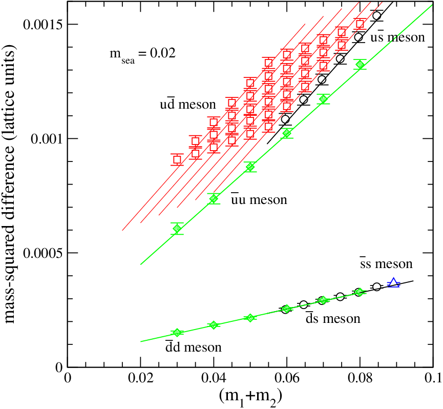
Now we turn to the determination of the quark masses. To this end, we extract the low-energy constants (LEC’s) defined in Sec. III.3 by fitting the difference of the square of the pseudoscalar mass with the same quantity evaluated at $\alpha=0$. The fits are uncorrelated since including the full covariance matrix makes them unstable, and it is likely ill-determined besides. Fitting all of the data at our disposal (61 masses at each sea quark mass), we find the LEC’s tabulated in Tab. 11. The mass squared differences and fit for $m_{sea}=0.02$ are shown in Fig. 6. Restricting the fit range to $m_{f}\leq 0.03$ does not change the values significantly as seen in Tab. 11, though the $\chi^{2}$/dof value is reduced. The corresponding $\alpha=0$ values of $B_{0}$ and the NLO Gasser-Leutwyler constants are given in Tab. 12.

The LEC’s in Eq. (33) are extracted using the mass dependence of the form $m_{i}+m_{res}$. Then the remaining explicit chiral symmetry breaking effects at order ${\cal O}(\alpha m_{res})$ are contained in the constants $\delta$ and $\delta_{m_{res}}$. The value of $\delta_{m_{res}}$ in Tab. 11 should be compared with the value of $C_{2}$ determined from $\Delta m_{res}$. In particular, one should have $\delta_{m_{res}}=2B_{0}C_{2}$. One sees that this combination is roughly two times too large. Since the LEC $\delta_{m_{res}}$ is found by linearly extrapolating to the chiral limit, it is possible that the discrepancy arises due to the omission of chiral logs. Recall that the logs are ${\cal O}(m_{q}\log m_{q})$ compared to the linear terms and so could make a difference. Also note that the value of $C_{2}$ is roughly an order of magnitude smaller than the physical $\delta$ LEC. Because $\delta$ and $C_{1}$ have the same charge dependence, it is their sum which is extracted from the fit. Thus, we must subtract off the amount $2B_{0}C_{1}$ from $\delta$ to obtain the physical LEC. This amounts to about a 20% reduction from the fitted value of $\delta$. Note that the higher order effects in the residual mass also affect the logarithms in Eqs. (26) and (28) which therefore do not cancel exactly in the meson mass-squared difference with QED switched on and off. However, these terms are order ${\cal O}(m\,\Delta m_{res})$ in the chiral expansion, so we neglect them.

The meson mass-squared splittings show little dependence on the sea quark mass. In Fig. 7 we show a representative sample of splittings for each sea quark mass. This is reasonable since we have not coupled the sea quarks to the photons, so the difference between ensembles is likely due to fluctuations in the gluon fields. In partially quenched chiral perturbation theory for 2+1 flavors Bijnens:2006mk, there exists a term at NLO that couples the valence quark charges to the sea quark masses. To account for this possibility, we include the $\delta_{sea}$ term in our fit (see Eq. (33), and notice that only the charged mesons are affected). From Tab. 11 we see $\delta_{sea}$ is small, consistent with zero for the fit range including all masses, and only two standard deviations away from zero for the reduced range, which includes only the lightest two sea quark masses. The values of the other LEC’s are largely unaffected by the $\delta_{sea}$ term, except $\delta$, which is reduced in the first case and increased in the second. Because the evidence is not strong in our data for such a term, we focus on the fits with $\delta_{sea}$ fixed to zero in the following.

Using the results for the LEC’s, we determine the quark masses as follows. As inputs, the three experimental values of $m_{\pi^{+}}^{2}$, $m_{K^{\pm}}^{2}$, and $m_{K^{0}}^{2}$ are taken. We avoid the $\pi^{0}$ since we have not determined its true mass to NLO due to the lack of disconnected diagrams. We then iteratively solve the set of equations generated from Eq. (35) for each meson for the three unknowns $m_{u}$, $m_{d}$, and $m_{s}$. At this stage, the quark masses are the bare lattice values, including the shift due to the residual mass.

Using the non-perturbatively determined quark mass renormalization constant $1/Z_{m}=Z_{S}$=0.62(4) RBC NP Zm, we obtain the values of the light quark masses, $m^{\overline{\rm MS}}(2{\rm GeV})=Z_{m}(m_{q}+m_{\rm res})$, and ratios shown in Tab. 13. The error on $Z_{S}$ reflects a statistical and a systematic error from the choice of $\Lambda_{QCD}$ in the range 250-300 MeV, which have been added in quadrature. As the bare quark mass range used in the fit to meson mass-squared is reduced from 0.0446 to 0.03, the physical quark masses change by about one statistical standard deviation, or less. The only change outside of one standard deviation is for the quark mass ratios which are determined very precisely. The ratio of up quark to down quark mass comes out to be close to one-half while the strange quark to average up-down quark mass is about 28 to 29, depending on the fit range.

Knowing the physical up and down quark masses, the physical charged-neutral pion mass splitting is found from the LEC’s in Tab. 11. Dividing the mass-squared difference by $m_{\pi^{+}}+m_{\pi^{0}}$, we find $m_{\pi^{+}}-m_{\pi^{0}}=3.89(17)$ MeV using all data, and 4.12(21) MeV using quark masses less than or equal to 0.03, which is somewhat less than the physical value of 4.5936 MeVYao:2006px. The part of this difference arising from the up-down quark mass difference was estimated a long time ago to be about 0.17(3) MeV Gasser:1984gg and more recently, 0.32 (20) MeV Bijnens:1996kk. In addition, there are still several systematic errors like non-zero lattice spacing and finite volume effects to be addressed in the calculation of the mass splitting, so the level of disagreement is not surprising, perhaps even encouraging. It is interesting to note that almost the entire mass difference comes from the leading term ($\sim 98\%$) since the physical up and down quark masses are so small (the omission of disconnected diagrams for the $\pi^{0}$ mass has a very small effect here). Similarly, we find the EM part of the kaon mass difference, $m_{K^{+}}-m_{K^{0}}=1.443(55)$ MeV for the resricted range (1.441(42) MeV for the whole range). QED effects make the charged kaon heavier, just as for the pions. In this case, the leading term also dominates, but the ${\cal O}(\alpha m_{s})$ terms contribute about 23%. Ultimately, the pure QCD $B_{0}(m_{u}-m_{d})$ term dominates the physical states and makes the neutral kaon heavier by 3.972(27) MeVYao:2006px.

From Eq. (34) the breaking of Dashen’s theorem at ${\cal O}(\alpha m_{q})$ is found to be $\Delta_{\rm EM}=0.337(40)$ or 0.264(43), using the restricted fit range. This is somewhat smaller than the large $N_{c}$ estimate reported in Bijnens:1996kk, $\Delta_{\rm EM}=0.85(24)$. Following Aubin:2004fs, $\Delta_{\rm EM}$ would have to be roughly 10 in our calculation to render the up quark massless.

We now turn to a discussion of the systematic errors in our calculation. In the calculation of the neutral pion correlation function, we ignored the contribution from disconnected diagrams. Disconnected diagrams contribute to $m_{\pi^{0}}^{2}$ (and $m_{\eta}^{2}$) at ${\cal O}(\alpha m_{q})$ ⁴⁴ 4 We have sought a proof that such contributions enter at ${\cal O}(\alpha m_{q}^{2})$. In fact, one can show the leading contribution, where only a single photon is exchanged between the quark loops, vanishes. Likewise, any diagram where one photon and any even number of gluons are exchanged also vanishes if one considers each quark loop to be made from renormalized propagators and vertices only. However, if more general diagrams are considered, like the above but including a gluon exchange between two separated quark propagators from the same loop, the proof no longer holds. In any case, we expect these contributions to be suppressed, at least in the weak coupling limit of QCD. so this is potentially a significant effect. However, we avoided using the $\pi^{0}$ mass to determine the quark masses, so this will not affect those estimates. And as mentioned above, the physical $\pi^{+}-\pi^{0}$ mass splitting is dominated by the LO contribution since the up and down quark masses are so small. The main effect would be to alter the value of the LEC $\delta_{0}$ for the $\pi^{0}$ and $\eta$ mesons which we have assumed has the same value for all pseudoscalar mesons.

In any study of the EM interactions, finite volume effects may be significant as the photons are massless (and unconfined). In order to get a rough estimate for the size of this effect, we examine the finite volume effect to $\delta$ using the vector-saturation model Das:1967it; Bardeen:1988zw; Ecker:1988te; Donoghue:1993hj; Harada:2004qn as an example⁵⁵ 5 More correctly, a parameter representing non-resonance contributions, which turns out to be small Ecker:1988te, is set to zero. . Assuming that the finite size effect purely due to QCD cancels in the difference between $m_{\pi^{+}}$ and $m_{\pi^{0}}$, this model estimates the mass difference in a finite volume, $\Delta_{\pi,\rm EM}=m_{\pi^{+}}^{2}-m_{\pi^{0}}^{2}$, to be

$$\Delta_{\pi,\rm EM}(L)=\frac{3\,\alpha}{4\pi}\,\frac{1}{a^{2}}\,\frac{2^{4}\cdot\pi^{2}}{N}\sum_{q\in\widetilde{\Gamma}^{\prime}}\frac{(am_{\rho})^{2}(am_{A})^{2}}{\widehat{q}^{\,2}\left(\widehat{q}^{\,2}+(am_{\rho})^{2}\right)\left(\widehat{q}^{\,2}+(am_{A})^{2}\right)}\,,$$

(48)

where $N$ is the total number of sites, $\widetilde{\Gamma}^{\prime}$ is the first Brillouin zone in the momentum space apart from $q_{\mu}=0$, and

	$\displaystyle\widehat{q}^{\,2}$	$\displaystyle\equiv$	$\displaystyle\sum_{\mu=0}^{3}\widehat{q}_{\mu}^{\,2}\,,$
	$\displaystyle\widehat{q}_{\mu}$	$\displaystyle\equiv$	$\displaystyle 2\,\sin\left(\frac{aq_{\mu}}{2}\right)\,.$		(49)

Applying our lattice volume and taking the ratio to that in the infinite volume, we obtain

$$\frac{\Delta_{\pi,\rm EM}(\infty)}{\Delta_{\pi,\rm EM}(L\approx 1.9\ {\rm fm})}=1.10\,.$$

(50)

Thus we find roughly a $+10$% increase in $\delta$. We expect a similar size of correction for the other $\delta_{i}$’s. The shift in $\delta$ could affect the determination of the quark masses. Shifting the value of physical $\delta-2B_{0}C_{1}$ by 10%, we find the quark masses change by less than 1%. Thus we conclude that the finite volume effect on the quark masses due to the EM interaction is negligible. However, removing this effect will enhance the pseudoscalar mass splitting itself significantly.

We did not take into account the renormalization of the quark masses due to the EM interaction. However, the QED part of the renormalization is expected to change the quark mass by ${\cal O}(\alpha)\sim 1\%$. Since this is well within the statistical and other uncertainties discussed already, we ignore this effect. In future calculations it will be a simple matter to include these effects directly in the non-perturbative renormalization calculation of $Z_{m}$.

The use of the quenched approximation for the QED gauge fields results in a leading error of order $\alpha\,\alpha_{S}^{2}$ in correlation functions since the dynamical quarks do not interact via the quenched photons. However, as noted in Bijnens:2006mk the sea quark charge effects that enter at ${\cal O}(\alpha m_{sea})$ can be dealt with in two ways. First, the log terms come with known coefficients so can be subtracted from the lattice results before fitting for the LEC’s. Second, the LEC’s which come with sea quark dependence cancel out of some mass squared differences. The latter is operable here but not the former since we did not fit to the chiral logs as they are not known for the $N_{f}=2$ partially quenched case. We expect sea quark effects to be small in this present study since they were treated explicitly as neutral particles with respect to the EM interaction.

Finally, we note that changing our bare quark mass fit range from 0.015-0.0446 (less than 1/2 $m_{s}$ to $m_{s}$) to 0.015-0.03 has little effect on the LEC’s or quark masses. Experience in the pure QCD case has shown that this range of quark masses is likely to be beyond the range of applicability of chiral perturbation theory Aoki:2004ht, and $\chi^{2}$/dof does decrease for the restricted range. So, being conservative, we take as central values those results determined from the pseudoscalar two-point function with a quark mass fit range $0.015\leq m_{f}\leq 0.03$. There is some uncertainty introduced by the inclusion of the LEC $\delta_{sea}$, which we set to zero or found to be small (or zero within errors) when left as a free parameter. Since the evidence is uncertain for such a term in our data, and the sea quarks are not charged, we stick with the fit with $\delta_{sea}=0$ to quote our results for the quark masses. Thus, from the third row of Tab. 13 our final values for the quark masses are

	$\displaystyle m^{\overline{\rm MS}}_{u}(2\,{\rm GeV})$	$\displaystyle=$	$\displaystyle 3.02(27)(19)\mbox{ MeV},$		(51)
	$\displaystyle m^{\overline{\rm MS}}_{d}(2\,{\rm GeV})$	$\displaystyle=$	$\displaystyle 5.49(20)(34)\mbox{ MeV},$		(52)
	$\displaystyle m^{\overline{\rm MS}}_{ud}(2\,{\rm GeV})$	$\displaystyle=$	$\displaystyle 4.25(23)(26)\mbox{ MeV},$		(53)
	$\displaystyle m^{\overline{\rm MS}}_{s}(2{\rm GeV})$	$\displaystyle=$	$\displaystyle 119.5(56)(74)\mbox{ MeV},$		(54)
	$\displaystyle m_{u}/m_{d}$	$\displaystyle=$	$\displaystyle 0.550(31),$		(55)
	$\displaystyle m_{s}/m_{ud}$	$\displaystyle=$	$\displaystyle 28.10(38).$		(56)

The first error is statistical, the second from the error on the renormalization constant $Z_{m}$.

References

- (1) C. T. H. Davies et al. [HPQCD Collaboration], Phys. Rev. Lett. 92, 022001 (2004) [arXiv:hep-lat/0304004].
- (2) T. Izubuchi, plenary review talk given at the XXIII International Symposium on Lattice Field Theory “Lattice 2005”, Dublin, PoS (Lattice 2005) 003.
- (3) L. Giusti, plenary review talk given at the XXIV International Symposium on Lattice Field Theory “Lattice 2006”, Tucson, PoS (Lattice 2006) 009.
- (4)
A. Duncan, E. Eichten and H. Thacker,
Phys. Rev. Lett. 76, (1996) 3894,
arXiv:hep-lat/9602005;
Nucl. Phys. Proc. Suppl. 53, (1997) 295, arXiv:hep-lat/9609015. - (5)
Phys. Lett. B 409, (1997) 387,
arXiv:hep-lat/9607032;
Nucl. Phys. Proc. Suppl. 53, (1997) 299, arXiv:hep-lat/9608143. - (6) D. B. Kaplan, Phys. Lett. B 288, (1992) 342, arXiv:hep-lat/9206013.
- (7) Y. Shamir, Nucl. Phys. B 406, (1993) 90, arXiv:hep-lat/9303005.
- (8) Y. Aoki et al., Phys. Rev. D 72, 114505 (2005) [arXiv:hep-lat/0411006].
- (9) A. Duncan, E. Eichten and R. Sedgewick, arXiv:hep-lat/0405014.
- (10) T. Das, G. S. Guralnik, V. S. Mathur, F. E. Low and J. E. Young, Phys. Rev. Lett. 18, (1967) 759.
- (11) W. A. Bardeen, J. Bijnens and J. M. Gerard, Phys. Rev. Lett. 62, (1989) 1343.
- (12) G. Ecker, J. Gasser, A. Pich and E. de Rafael, Nucl. Phys. B 321, (1989) 311.
- (13) J. F. Donoghue, B. R. Holstein and D. Wyler, Phys. Rev. D 47, (1993) 2089.
- (14) M. Harada, M. Kurachi and K. Yamawaki, Phys. Rev. D 70 (2004) 033009, arXiv:hep-ph/0403120.
- (15) M. Hayakawa, T, Blum, T. Izubuchi and N. Yamada, PoS(LAT2005) 353, [arXiv:hep-lat/0509016].
- (16) N. Yamada, T. Blum, M. Hayakawa and T. Izubuchi [RBC Collaboration], PoS LAT2005, 092 (2006) [arXiv:hep-lat/0509124].
- (17) Y. Namekawa and Y. Kikukawa, PoS LAT2005, 090 (2006) [arXiv:hep-lat/0509120].
- (18) D. J. Gross, S. B. Treiman and F. Wilczek, Phys. Rev. D 19, 2188 (1979).
- (19) J. Gasser and H. Leutwyler, Nucl. Phys. B 250, (1985) 465.
- (20) V. Furman and Y. Shamir, Nucl. Phys. B 439, 54 (1995) [arXiv:hep-lat/9405004].
- (21) For example, see, Y. Shamir, Nucl. Phys. B 417, 167 (1994) [arXiv:hep-lat/9310006].
- (22) M. F. L. Golterman and K. C. L. Leung, Phys. Rev. D 57, 5703 (1998) [arXiv:hep-lat/9711033].
- (23) J. Laiho and A. Soni, Phys. Rev. D 65, 114020 (2002) [arXiv:hep-ph/0203106].
- (24) J. Gasser and H. Leutwyler, Annals Phys. 158, 142 (1984).
- (25) R. Urech, Nucl. Phys. B 433, 234 (1995) [arXiv:hep-ph/9405341].
- (26) J. Bijnens and N. Danielsson, arXiv:hep-lat/0610127.
- (27) J. Bijnens and J. Prades, Nucl. Phys. B 490, 239 (1997) [arXiv:hep-ph/9610360].
- (28) R. F. Dashen, Phys. Rev. 183, 1245 (1969).
- (29) C. Aubin et al. [MILC Collaboration], Phys. Rev. D 70, 114501 (2004) [arXiv:hep-lat/0407028].
- (30) T. Blum, Nucl. Phys. Proc. Suppl. 73, 167 (1999) [arXiv:hep-lat/9810017].
- (31) T. Blum et al., Phys. Rev. D 69, 074502 (2004) [arXiv:hep-lat/0007038].
- (32) W. M. Yao et al. [Particle Data Group], J. Phys. G 33, 1 (2006).
- (33) C. Dawson and T. Izubuchi [RBC collaboration], in preparation.
- (34) T. Doi, T. Blum, M. Hayakawa, T. Izubuchi and N. Yamada, arXiv:hep-lat/0610095.
- (35) C. Allton et al. [RBC-UKQCD Collaboration], arXiv:hep-lat/0701013.
- (36) C. Allton et al. [RBC-UKQCD Collaboration], in preparation.