Holographic Nuclear Physics
Abstract:
We analyze the phases of the Sakai-Sugimoto model at finite temperature and baryon chemical potential. Baryonic matter is represented either by 4-branes in the 8-branes or by strings stretched from the 8-branes to the horizon. We find the explicit configurations and use them to determine the phase diagram and equation of state of the model. The 4-brane configuration (nuclear matter) is always preferred to the string configuration (quark matter), and the latter is also unstable to density fluctuations. In the deconfined phase the phase diagram has three regions corresponding to the vacuum, quark-gluon plasma, and nuclear matter, with a first-order and a second-order phase transition separating the phases. We find that for a large baryon number density, and at low temperatures, the dominant phase has broken chiral symmetry. This is in qualitative agreement with studies of QCD at high density.
1 Introduction
QCD at finite baryon density has a rich phase structure (for reviews see [1, 2, 3]). Naively one would expect that at high density, like at high temperature, QCD is in a deconfined chiral-symmetric quark-gluon plasma phase. It turns out, however, that new phases appear at high density, in which both the chiral symmetry and the gauge symmetry are broken [2, 3]. In real QCD with and three light flavors of quarks the dominant phase at high density is a color-flavor-locking (CFL) phase [4]. With two light flavors of quarks the dominant phase is a color-superconductor. At large it is believed that these gauge-symmetry breaking phases are suppressed, and the dominant phase at high density is a chiral density wave [5, 6], in which the chiral symmetry (only) is broken non-uniformly. It appears therefore that QCD (both with and at large ) at low temperature and high density always has broken chiral symmetry.
These results rely on perturbative calculations in QCD, and analogous models such as the Nambu-Jona-Lasinio (NJL) model, at finite density near the Fermi surface, and are therefore limited to values of the chemical potential for which . At present, lattice QCD techniques are unable to deal with a (large) baryon chemical potential (for a review see [7]).
At large , gauge/gravity duality is an alternative approach to gauge theory at strong coupling [8]. Several recent models have incorporated flavors using probe branes in backgrounds dual to large Yang-Mills theories with various amounts of supersymmetry [9]. The Sakai-Sugimoto model in particular is quite similar to QCD at large [10]. This model builds on Witten’s model for pure Yang-Mills theory in four dimensions, which uses 4-branes wrapped on a Scherk-Schwarz circle [11], and adds probe 8-branes and probe anti-8-branes transverse to the circle. These provide massless chiral fermions (left-handed from the 8-branes, right-handed from the anti-8-branes) in the fundamental representation of both the gauge group , and the flavor group .
One of the most compelling features of this model is that it describes spontaneous chiral-symmetry breaking in a simple geometrical way. Since in the near-horizon limit the circle vanishes at a finite radial coordinate, the 8-branes and anti-8-branes are smoothly connected into a U-shaped configuration with an asymptotic separation at infinity. The actual embedding of the 8-branes is determined by solving the DBI equations of motion with this boundary condition.
The model also exhibits many other properties similar to QCD [12, 13]. In particular it has an interesting phase structure at finite temperature [14]. At low temperature the model is essentially the same as at zero temperature, i.e. it describes a confining gauge theory with broken chiral symmetry. At high temperature the model deconfines and chiral symmetry is restored, which is described geometrically by the separation of the 8-branes and anti-8-branes. For sufficiently small there is also an intermediate range of temperatures at which the model is deconfined but chiral symmetry remains broken. In the deconfined phase both the connected U-configuration and the separated parallel configuration are possible. The dominant configuration, and therefore phase, is determined by comparing their actions.
The baryonic symmetry corresponds in models with fundamental matter to the diagonal gauge symmetry of the probe branes. Baryon number is therefore described by electric charge, and baryon number density is related to the electric field, or more precisely to the electric displacement field, of the diagonal . Correspondingly, the baryon chemical potential is described by the value of the gauge potential at infinity . Finite baryon density in the Sakai-Sugimoto model has been studied in [15, 16, 17, 18]. However, only part of the parameter space has been explored so far. Other models with finite baryon density have been studied in [19, 20, 21, 22].
In this paper we explore the full parameter space of the Sakai-Sugimoto model at finite temperature and finite uniform baryon number density, in both the confined and deconfined phases. Other than temperature and baryon number density (or chemical potential), this model has an additional parameter not present in QCD, namely the asymptotic 8-brane-anti-8-brane separation . We will assume that the value of is such that the intermediate phase of deconfinement with chiral symmetry breaking exists, in other words that the deconfinement temperature is (much) smaller than the chiral-symmetry restoration temperature. The confined phase is, of course, of great interest, but the deconfined phase exhibits a much richer phase diagram. The deconfined phase is also qualitatively the same as the non-local NJL model [23, 24], and we expect a similar phase diagram in that case.
There are two types of objects which carry baryon charge. The baryons themselves correspond to 4-branes wrapped on the part of the background. Due to the RR flux each 4-brane comes with strings attached [25]. The other end of the strings is attached to the 8-branes, which is how the baryons get their flavor. However, in the nonsupersymmetric 4-brane background this configuration is not static. The strings pull the wrapped 4-branes up toward the 8-branes [26]. When they reach the 8-branes, the 4-branes can also be described as instantons in the world-volume theory of the 8-branes. In the deconfined phase baryon charge can also be carried by strings which stretch from the 8-branes all the way to the horizon.11 1 We can think of these strings as ending on massless, wrapped 4-branes at the horizon. This describes a possible phase in which baryon charge is carried by free quarks.
In both cases we will consider a uniform distribution in of baryon charge, so the 8-brane worldvolume theory reduces to a one-dimensional problem in the radial coordinate with a source term. As the 4-branes and strings exert a force on the 8-branes, their embedding at finite baryon number density will have a cusp.
We will make the following approximations. First, we will assume that the wrapped 4-branes are pointlike in the transverse coordinates and uniformly distributed in . The precise description would be in terms of instantons in the 8-brane worldvolume theory. However, instanton solutions in DBI are not known. Analysis in the Yang-Mills (plus Chern-Simons) approximation shows that an instanton has a finite size on the order of the string length [13]. Using pointlike instantons, or equivalently pointlike 4-branes, is therefore a good approximation. We will also neglect any direct interactions between the 4-branes themselves or between the strings.
Our results are summarized in the phase diagram in figure 1. At low temperatures the theory confines, and there is a second order phase transition at finite to a phase of nuclear matter. At high temperature the theory deconfines and chiral symmetry is restored. At intermediate temperatures chiral symmetry is broken for all (as in QCD). We find a second order phase transition also in the intermediate temperature range between the vacuum and nuclear matter phases. This is similar to QCD, but in QCD it is a first-order transition due to the attractive interaction between the baryons (which we have neglected).

In section 2 we begin by describing the possible 8-brane configurations corresponding to the Sakai-Sugimoto model at finite baryon number density. In section 3 we discuss the thermodynamics of the gauge theory which are implied by these configurations and derive the full phase diagram in the grand canonical ensemble. We consider both the confined and deconfined phases, and both 4-branes and strings as sources of baryon charge in the deconfined phase. It will turn out that 4-branes are always preferred to strings, and that the stringy “quark matter” phase is actually unstable to density fluctuations. We conclude and offer suggestions for future work in section 4.
2 Finite density brane configurations
The basic brane configuration consists of 8-branes and anti-8-branes in the near horizon background of 4-branes wrapped on a Scherk-Schwarz circle with . At zero temperature the background is capped and the circle is topologically trivial, so the 8-branes and anti-8-branes connect into a U-shaped configuration. The dual gauge theory is confining, and chiral symmetry is broken. At finite temperature this continues to be the only possible configuration until one reaches a critical temperature, at which the dominant background switches to the black hole, and both U-shaped 8-branes and separated parallel 8-branes and anti-8-branes are allowed. At first the U-shaped configuration dominates, so chiral symmetry remains broken even though the gauge theory deconfines. Chiral symmetry restoration occurs at a second critical temperature, which for small enough, is above the first critical temperature (otherwise they are equal). At this temperature the separated 8-brane-anti-8-brane configuration begins to dominate.
The baryon number current is related holographically to the diagonal part of the 8-brane gauge field. To study finite baryon number density configurations we therefore need to include this gauge field in the 8-brane action. The first place it enters is in the DBI action:
| (1) |
where is the field strength
| (2) |
We decompose the gauge field into an part and a part as follows22 2 We are using the convention .
| (3) |
The gauge field will also appear in the CS action, which will be important below. Let’s study the effect of turning on this gauge field on the brane configuration in the different phases.
2.1 confined phase
In the confined phase the background (at finite temperature) is given by
| (4) | |||||
| (5) | |||||
| (6) |
where , , and
| (7) |
It is convenient to express everything in terms of dimensionless quanitities, so we define
| (8) |
The 8-brane action with the gauge field is then given by33 3 This is the action for just the 8-branes, i.e. for 1/2 of the full configuration. The lower limit of the integral is the lowest radial position of the 8-brane configuration, and the upper limit is infinity.
| (9) |
where we have defined the overall normalization as
| (10) |
where is the volume of a unit , and is the volume of space (). Note that the action scales as .
As will become clear in the next section it is convenient to also define the Legendre-transformed action
| (11) |
where is the electric displacement field defined by
| (12) |
This gives
| (13) |
The equations of motion for and can be integrated once yielding two constants:
| (14) |
where is defined as the position where diverges.
For the solution is a U-shaped 8-brane in the plane, with as its lowest radial position (figure 2) [10]. However, a non-trivial electric displacement requires a source at , which is possibly different from , which will change the 8-brane configuration. This is essentially a one-dimensional electrostatics problem in the coordinate , except that the 8-brane covers the region twice. Each part carries an electric displacement .
The only possible sources for in the confined phase are instantons, or equivalently 4-branes wrapped on the , in the 8-branes. For a uniform we need a uniform distribution in of 4-branes. The source term comes from the 8-brane CS action:
| (15) |
The relevant term is the one that couples the to the :
| (16) |
We will assume a uniform distribution of 4-branes in at :
| (17) |
where is the (dimensionless) density of 4-branes wrapped on . The equation of motion for the gauge field then gives
| (18) |
and therefore44 4 This is the density of 4-branes on one half of the 8-brane configuration. The total 4-brane density is twice this much.
| (19) |
The instanton distribution (17) also sources the equation of motion for and will therefore deform the shape of the 8-brane. Physically, the 4-branes pull down on the 8-branes. Since the 4-brane distribution has a finite energy density per unit 7-volume (the they wrap plus the ), it will form a cusp in the 8-brane (like a bead on a string). Away from the cusp the 8-brane will follow two opposite pieces of a U-shaped solution, which are truncated at some radial position above (figure 2).


The value of can determined by the zero-force condition in the plane. The proper tension of the 8-brane is given by varying the Legendre-transformed action (13) (which is the same as the Hamiltonian once we substitute in for the solution of ) with repsect to the proper distance along the 8-brane. The result is
| (20) |
The force due to the 4-branes is given simply by varying their action with respect to their position , again taking care to vary with respect to the proper distance. The 4-brane action is
| (21) | |||||
and the force is therefore
| (22) |
The condition for equilibrium is then
| (23) |
where is the proper angle of the 8-brane at ,
| (24) |
An elegant alternative derivation of this result is given in the Appendix.
We want to solve this for , while holding fixed the asymptotic separation of the 8-branes and anti-8-branes, which is given by
| (25) |
This can be done numerically by varying and , computing and using (23) and (25), and then tabulating for a given value of . The result is presented in figure 3, where for definiteness we have set . Note that for small values of the cusp comes down as increases, but beyond a certain value of it goes up. Initially the 4-branes pull the 8-branes down, but eventually the 8-branes win this “tug-of-war”. We will see the same behavior in the deconfined phase. The initial downward motion of the cusp indicates that the chiral condensate of the gauge theory decreases initially as the density increases, and the eventual upward motion indicates that the chiral condensate eventually increases with . As we will soon see this has an important implication for the gauge theory thermodynamics at high density.

2.2 deconfined phase
The background describing the deconfined phase is given by exchanging the roles of and :
| (26) |
with the same dilaton and RR 4-form as before, and where
| (27) |
where is the dimensionless temperature. The 8-brane action is now given by
| (28) |
and the Legendre-transformed action is
| (29) |
where is now given by
| (30) |
As in the confined phase, the equation of motion for implies that it is a constant . On the other hand, for there are two types of possible configurations (figure 4). The first corresponds to separated parallel 8-branes and anti-8-branes with
| (31) |
and the second to a connected configuration with
| (32) |
Actually, as we will soon see there are in fact two connected solutions, but only one is (classically) stable.


2.2.1 4-brane sources
The parallel configuration can have a uniform electric displacement without sources. In the connected configuration, however, we need a source, as in the confined phase. One possible source is again 4-branes inside the 8-branes. The 4-brane action is now
| (33) |
and the force they exert is given by
| (34) |
where in the last equality we used the form of in (27). The 8-brane force is computed as before, but with the metric of the deconfined phase. This gives
| (35) |
and the same angle as before (24). The solution of the zero-force condition for a representative temperature is shown in figure 5. The qualitative behavior is the same as in the confined phase: initially the cusp comes down as increases, but eventually it goes up and approaches a fixed value.

In the deconfined phase there are actually two connected solutions in general. This can be seen by looking at as a function of the cusp position at fixed and (figure 6). There are two values of for a given below some . At the two solutions coincide, and above there is no connected solution. This behavior is also true for . So in fact there are three solutions in all when : the parallel configuration, a “short” cusp configuration (or “short” U-configuration when ), and a “long” cusp configuration (or “long” U-configuration when ). When only the parallel configuration is a solution. This picture is very reasonable from the following point of view. Imagine that we have two classically stable solutions in some theory with a potential. The two solutions correspond to two local minima of the potential. But this necessarily implies that there should be a third solution, corresponding to the local maximum between the two minima (figure 7a). This solution should be unstable. Now imagine that one local minimum is lower than the other, and that the second local minimum approaches the local maximum as we vary some parameter. When they coincide we get a point of inflection (figure 7b). As we continue to vary the same parameter both solutions cease to exist, leaving only the lower minimum (figure 7c). This is precisely what happens for the 8-brane embedding. The parallel and short cusp configurations are the stable solutions. The long cusp configuration must therefore correspond to the unstable solution. We leave it as a future excercise to exhibit the required negative mode. Note that this picture necessarily implies that we don’t have to worry about the cusp solution disappearing, since in the region of parameter space near this point the parallel solution always dominates.


2.2.2 string sources
The other possible sources of electric displacement in this phase are strings which stretch from the 8-branes to the horizon at .55 5 Instead of ending at the horizon, the strings may also end on 4-branes which wrap the and are located below the 8-branes. This is Witten’s description of baryons [25]. Each 4-brane has strings attached to it. However this configuration is not a solution of the equations of motion. There is a net force that pulls the 4-brane to larger [26]. Eventually the 4-brane reaches the 8-brane and turns into an instanton. We can determine the precise relation between the density of strings and the electric displacement by looking at the -field dependence of the supergravity, 8-brane, and string actions:
| (36) | |||||
| (37) | |||||
| (38) |
Varying with respect to and integrating over an 8-sphere surrounding the endpoint of the strings in the 8-branes we find that
| (39) |
Note that this is consistent with what we found for 4-branes in (19), since each 4-brane (away from the 8-branes) has strings attached.
Evaluating the string action for the deconfined background gives
| (40) |
As in the 4-brane case, we have assumed a uniform distribution of strings in , so the point on the 8-brane where they end will again be a cusp. The force downward applied by the strings is given by
| (41) |
The solution to the zero-force condition with the strings is shown in figure 8. The behavior is different from the 4-brane case. The position of the cusp comes down monotonically with increasing .

It turns out, however, that the stringy cusp configuration is always subdominant to the 4-brane cusp configuration. We can see this by comparing their actions. The total action will have a contribution from the 8-branes given by (29), where the integral is taken from to infinity, and from either the 4-brane or string sources. The integrals are divergent, but we can regularize them by subtracting the action of the 8-branes in the parallel configuration in both cases. The results are shown in figure 9. The action of the cusp configuration sourced by 4-branes is smaller than that of the configuration sourced by strings at all temperatures and for all values of .


In the next section we will show that in fact this configuration is unstable to fluctuations in . This is similar to the instability found in [19]. We will comment on a possible interpretation of this instability in the conclusions.
3 Thermodynamics with finite chemical potential
We now turn to the gauge theory implications of the configurations we found. Our main goal is to understand the phase diagram of the gauge theory at finite temperature and finite baryon chemical potential . Note that this model has an additional parameter not present in QCD corresponding to the asymptotic 8-brane-anti-8-brane separation . We will generally fix . We have also considered other values of (smaller and larger) and found no qualitative change in the results.
3.1 baryon chemical potential
The grand canonical potential is obtained by evaluating the 8-brane action (9) or (28) on the solution. For convenience we will normalize the potential by dividing out the normalization constant ,
| (42) |
Note however that the potential, as well as all other thermodynamic quantities associated to the matter, scale as . The (dimensionless) baryon chemical potential is identified with the asymptotic value of the gauge potential in the solution
| (43) |
With our normalizations the baryon number density is given by66 6 The true baryon number density is given by (19).
| (44) |
We will therefore use to denote also the density.
For computational purposes it is more convenient to express in terms of using the canonical ensemble. The free energy is defined as
| (45) |
and the chemical potential is given by
| (46) |
The free energy is thus related to the Legendre-transformed 8-brane action on the solution. In the cusp configuration the total free energy includes also the contribution of the source 4-branes or strings, evaluated at the position of the cusp:
| (47) |
The dependence on comes from three places: the explicit dependence of and on , the dependence of the solution for on , and the dependence on of . Including all of these gives
| (48) | |||||
The second term vanishes since is constant by the equation of motion for and the integral of , at fixed , gives which vanishes since is fixed. The third and fourth terms cancel by the zero-force condition at the cusp (see Appendix), leaving
| (49) |
where is related to by inverting the relation (12) or (30). The identification of the chemical potential with the value of the gauge potential at infinity (43) therefore reflects a particular choice of gauge, in which is identified with the mass of the source. In the parallel configuration the source term vanishes, and the lower limit of the integral is at the horizon . In this case the gauge choice (43) gives , which is consistent with the fact that the source becomes massless at the horizon.
3.2 confined phase
In the confined phase only a connected 8-brane configuration is possible. However for a given , that is at fixed , there are two connected solutions, a U-configuration with and a 4-brane sourced cusp configuration with . The former corresponds to the QCD vacuum, and the latter to a phase of nuclear matter. In the vacuum phase is constant, and the electric displacement vanishes. Therefore does not depend on in this phase. In the nuclear matter phase is sourced by 4-branes, and the chemical potential is given by (49), which in the confined phase yields
| (50) |
Note that both and depend on and . There is no temperature dependence in the confined phase. As we are working in the grand canonical ensemble, this represents an implicit expression for . We see that there is a critical value for the chemical potential for which . Below this value there is no cusp solution and therefore no nuclear matter phase. This is precisely the onset chemical potential . For both the vacuum and the nuclear matter phases exist, and we must compare their grand canonical potentials to determine which phase is preferred. These quantities are actually divergent at , but the difference is finite and is given by
| (51) | |||||
where and are the (different) values of in the nuclear and vacuum phases, respectively. The results, for the representative value (and ), are shown in figure 10. Since for all , the nuclear matter phase is preferred. Figure 10 also shows the baryon number density as a function of the chemical potential for . (The value of grows with ). Near the density is continuous and behaves as . This is therefore a second-order phase transition with a critical exponent of 1. This is a reasonable result given our approximation of ignoring the baryon interactions.


3.3 deconfined phase
In the deconfined phase the situation becomes more interesting since there are more possible configurations at a given value of . In addition to the U-shaped and 4-brane-cusp configurations, there are the parallel configuration, with vanishing or non-vanishing density, and the string-cusp configuration. The parallel configuration corresponds to a phase in which chiral symmetry is restored. At finite density this is the quark-gluon plasma (QGP). The vacuum parallel configuration is irrelevant, since it is clear from (28) that a non-trivial is always preferred in the parallel configuration. The string-cusp configuration features strings stretched between the 8-branes and the horizon. We will refer to the corresponding phase in the gauge theory as quark matter. However, as we shall soon see this configuration is actually unstable, at least for a uniform distribution of baryon charge. That leaves three phases to compare: the vacuum (U-configuration), nuclear matter (4-brane-cusp) and the QGP (finite density parallel configuration). We therefore expect in general a phase diagram in the plane with three phase regions.
3.3.1 unstable quark matter
Let us first show that the quark matter phase (string-cusp configuration) is thermodynamically unstable. Evaluating the chemical potential (49) in the deconfined phase with string sources (40) yields
| (52) |
Figure 11 shows a plot of vs. for this configuration.
It is apparent that
| (53) |
(or equivalently in the canonical ensemble) and therefore that the string-cusp configuration is thermodynamically unstable to density fluctuations. A similar instability was found in the D3-D7 model at finite density [19].
3.3.2 phase diagram
We begin by comparing the vacuum phase to the QGP phase. The vacuum phase is described by the U-configuration, and the quark-gluon plasma (QGP) phase is described by the parallel configuration. The grand canonical potential of the vacuum can be read off from (28) and (32) with :
| (54) |
The potential of the QGP is given by (28) and (30) with :
| (55) |
The density is a function of which is obtained from (49) without sources, and (30). This gives
| (56) |
which can be inverted numerically to get . Both potentials are divergent at but the difference is finite:
| (57) |
Figure 12 shows for a few representative temperatures (and ). The transition between the two phases occurs when . We find a line of transitions between these two phases in the plane shown in figure 12. This result was obtained previously in [16].


We now turn to the comparison of the vacuum phase with the nuclear matter phase. We did this already in the confined phase, and found a second-order phase transition at some . Since the Sakai-Sugimoto model exhibits chiral-symmetry breaking also in the deconfined phase, it is reasonable to expect that nuclear matter should form also in this case. The potential of the nuclear phase (with 4-branes) is given by
| (58) |
where is again given implicitly in terms of using (49) with 4-brane sources:
| (59) |
We are now interested in the difference between the potentials of the nuclear phase and the vacuum phase,
| (60) |
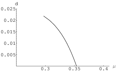
Figure 13 shows for a representative temperature. The behavior is qualitatively the same at all temperatures: is negative for all for which the nuclear phase exists. Figure 13 also shows the density as a function of at the same temperature. As in the confined phase, the critical exponent is 1 to within our numerical accuracy, so the transition is second order. By varying the temperature we obtain the phase diagram in figure 14. The behavior agrees qualitatively with what is expected in QCD: decreases slightly as the temperature increases.


The final part of the phase diagram comes from comparing the nuclear and QGP phases:
| (61) |
Here we find an interesting temperature dependence. Figure 15 shows for three representative temperatures. At low temperature the nuclear matter phase wins for all . Then there is a temperature range for which the system undergoes two transitions as is increased, first from nuclear matter to QGP, and then back to nuclear matter. The resulting phase diagram is shown in figure 15. The physical source of the dip in the phase diagram is the dip that occurs in the position of the cusp as a function of the density (figure 5). There is a similar dip in the phase diagram of QCD (see for example [3]). At high temperature (not shown) the QGP phase is preferred for all .
Finally, combining the three separate phase diagrams gives the complete phase diagram shown in figure 1. At low temperature and chemical potential the vacuum phase dominates, at low temperature and high chemical potential the nuclear phase dominates, and at high temperature chiral symmetry is restored and the quark-gluon plasma phase dominates.


3.4 entropy and equation of state
Phases of thermodynamic systems are also characterized by the their equation of state and entropy. Let us briefly discuss these for the different phases we have encountered.
The pressure as a function of the density is essentially given by . We find that at low temperature the behavior in the confined and deconfined phases is very similar.77 7 The behavior at high temperature, i.e. in the QGP phase, was essentially worked out in [24]. At small densities and therefore88 8 For a free fermi gas .
| (62) |
At large densities (figure 16) and thus
| (63) |
It is interesting that although we have not specified that the baryons are fermions (indeed there seem to be both fermionic and bosonic components), the results for mimic a behavior expected for fermions. This is due to the response of the DBI action to the electric field.


The entropy as a function of the temperature is computed from the free-energy . The interesting case is the deconfined phase, since there is no temperature dependence in the confined phase. At low temperature, where chiral symmetry is broken, we find (for both small and large densities)
| (64) |
and at the high temperature, where chiral symmetry is restored, we find
| (65) |
4 Conclusions
In this paper we have analyzed the different phases of the Sakai-Sugimoto model at finite temperature and baryon chemical potential and determined the phase diagram. In many respects our phase diagram is similar to that of QCD. In both cases chiral symmetry is broken at low temperature and restored at high temperature, at all values of the chemical potential. The dip in the phase diagram suggests that the chiral condensate initially decreases with and then increases. This is similar to the behavior in QCD. It would be interesting to study this directly using the holographic description of the chiral condensate in terms of the tachyon [27].
The finite density phase is described by a gas of ”baryonic matter” 4-branes wrapped on the inside the 8-branes. At low temperatures this phase always dominates over the quark-gluon plasma phase. The other possible description of baryon matter in terms of strings (”quark matter”) turns out to be subdominant and unstable. If we ignore these facts and use strings instead of 4-branes to describe baryonic matter the phase diagram would change and chiral symmetry would be restored at high density.
We also find a phase transition between the vacuum and nuclear matter phases. In QCD this is a first-order transition, but in our case it is second-order. We believe that that the difference is a result of neglecting the interactions between the 4-branes.
Another difference is that QCD at high density is expected to be in a CFL phase, in which both the chiral symmetry and the gauge symmetry are broken. However, at large QCD is expected to be dominated by a non-uniform chiral symmetry breaking phase with unbroken gauge symmetry. We did not explore this possibility in this paper. However the result that the “quark matter” phase, with strings stretched to the horizon, was unstable to density fluctuations, suggests that there may exist a stable non-unifrom phase. It would be interesting to see if it is similar to the chiral density wave in large QCD.
Appendix A Zero-force condition from the action
The force balance condition for the cusp configurations can alternately be obtained directly by varying the total action with respect to the cusp position . The total action is given by
| (66) |
We want to vary the action with respect to , while keeping the physical varaibles and fixed. To do this we need to vary (and therefore ) accordingly. This gives
| (67) |
However since is given by
| (68) |
we get
| (69) |
Furthermore, the equation of motion sets to a constant independent of . Requiring the total action to be stationary with respect to the varaition of one gets
| (70) |
Substituting in the expressions for and then reproduces the force balance conditions in the various cases (confined, deconfined, 4-branes, strings).
Acknowledgments
We would like to thank Ofer Aharony, David J. Bergman, Sumit Das, Ben Freivogel, Yariv Kafri, Keh-Fei Liu, David Mateos, Rob Myers, Al Shapere, Cobi Sonnenschein and Shigeki Sugimoto for helpful conversations. This work was supported in part by the Israel Science Foundation under grant no. 568/05.
References
- [1] T. Schafer, arXiv:hep-ph/0509068.
- [2] M. G. Alford, PoS LAT2006, 001 (2006) [arXiv:hep-lat/0610046].
- [3] K. Rajagopal and F. Wilczek, arXiv:hep-ph/0011333.
- [4] M. G. Alford, K. Rajagopal and F. Wilczek, Nucl. Phys. B 537, 443 (1999) [arXiv:hep-ph/9804403].
- [5] D. V. Deryagin, D. Y. Grigoriev and V. A. Rubakov, Int. J. Mod. Phys. A 7 (1992) 659.
- [6] E. Shuster and D. T. Son, Nucl. Phys. B 573, 434 (2000) [arXiv:hep-ph/9905448].
- [7] M. P. Lombardo, PoS C POD2006, 003 (2006) [arXiv:hep-lat/0612017].
- [8] O. Aharony, S. S. Gubser, J. M. Maldacena, H. Ooguri and Y. Oz, Phys. Rept. 323, 183 (2000) [arXiv:hep-th/9905111].
- [9] A. Karch and E. Katz, JHEP 0206, 043 (2002) [arXiv:hep-th/0205236]; T. Sakai and J. Sonnenschein, JHEP 0309, 047 (2003) [arXiv:hep-th/0305049]; J. Babington, J. Erdmenger, N. J. Evans, Z. Guralnik and I. Kirsch, Phys. Rev. D 69, 066007 (2004) [arXiv:hep-th/0306018]; X. J. Wang and S. Hu, JHEP 0309, 017 (2003) [arXiv:hep-th/0307218]; P. Ouyang, Nucl. Phys. B 699, 207 (2004) [arXiv:hep-th/0311084]; C. Nunez, A. Paredes and A. V. Ramallo, JHEP 0312, 024 (2003) [arXiv:hep-th/0311201]; M. Kruczenski, D. Mateos, R. C. Myers and D. J. Winters, JHEP 0405, 041 (2004) [arXiv:hep-th/0311270]; N. J. Evans and J. P. Shock, Phys. Rev. D 70, 046002 (2004) [arXiv:hep-th/0403279]; R. Casero, A. Paredes and J. Sonnenschein, JHEP 0601, 127 (2006) [arXiv:hep-th/0510110].
- [10] T. Sakai and S. Sugimoto, Prog. Theor. Phys. 113, 843 (2005) [arXiv:hep-th/0412141].
- [11] E. Witten, Adv. Theor. Math. Phys. 2, 505 (1998) [arXiv:hep-th/9803131].
- [12] T. Sakai and S. Sugimoto, Prog. Theor. Phys. 114, 1083 (2006) [arXiv:hep-th/0507073]; K. Peeters, J. Sonnenschein and M. Zamaklar, JHEP 0602, 009 (2006) [arXiv:hep-th/0511044]; P. Benincasa and A. Buchel, Phys. Lett. B 640, 108 (2006) [arXiv:hep-th/0605076]; K. Peeters, J. Sonnenschein and M. Zamaklar, Phys. Rev. D 74, 106008 (2006) [arXiv:hep-th/0606195]; Y. h. Gao, W. s. Xu and D. f. Zeng, arXiv:hep-th/0611217. K. Nawa, H. Suganuma and T. Kojo, Phys. Rev. D 75, 086003 (2007) [arXiv:hep-th/0612187]; O. Bergman and G. Lifschytz, JHEP 0704, 043 (2007) [arXiv:hep-th/0612289]; K. Nawa, H. Suganuma and T. Kojo, arXiv:hep-th/0701007; D. K. Hong, M. Rho, H. U. Yee and P. Yi, arXiv:hep-th/0701276; K. Hashimoto, T. Hirayama and A. Miwa, JHEP 0706, 020 (2007) [arXiv:hep-th/0703024]; D. K. Hong, M. Rho, H. U. Yee and P. Yi, arXiv:0705.2632 [hep-th].
- [13] H. Hata, T. Sakai, S. Sugimoto and S. Yamato, arXiv:hep-th/0701280;
- [14] O. Aharony, J. Sonnenschein and S. Yankielowicz, arXiv:hep-th/0604161.
- [15] K. Y. Kim, S. J. Sin and I. Zahed, arXiv:hep-th/0608046;
- [16] N. Horigome and Y. Tanii, JHEP 0701, 072 (2007) [arXiv:hep-th/0608198].
- [17] S. J. Sin, arXiv:0707.2719 [hep-th].
- [18] D. Yamada, arXiv:0707.0101 [hep-th].
- [19] S. Kobayashi, D. Mateos, S. Matsuura, R. C. Myers and R. M. Thomson, JHEP 0702, 016 (2007) [arXiv:hep-th/0611099].
- [20] S. K. Domokos and J. A. Harvey, arXiv:0704.1604 [hep-ph].
- [21] Y. Kim, B. H. Lee, S. Nam, C. Park and S. J. Sin, arXiv:0706.2525 [hep-ph].
- [22] Y. Kim, C. H. Lee and H. U. Yee, arXiv:0707.2637 [hep-ph].
- [23] E. Antonyan, J. A. Harvey, S. Jensen and D. Kutasov, arXiv:hep-th/0604017; A. Parnachev and D. A. Sahakyan, Phys. Rev. Lett. 97, 111601 (2006) [arXiv:hep-th/0604173];
- [24] A. Parnachev and D. A. Sahakyan, Nucl. Phys. B 768, 177 (2007) [arXiv:hep-th/0610247].
- [25] E. Witten, JHEP 9807, 006 (1998) [arXiv:hep-th/9805112].
- [26] C. G. . Callan, A. Guijosa, K. G. Savvidy and O. Tafjord, Nucl. Phys. B 555, 183 (1999) [arXiv:hep-th/9902197].
- [27] O. Bergman, J. Sonnenschein, S. Seki, to appear.