Blind background prediction using a bifurcated analysis scheme

We begin discussing this method in the case of a single background source. Here a collection of setup cuts have been applied which eliminate all other sources of background. Our goal is to predict the amount of background in the signal region when we apply the cuts $A$ and $B$, which we refer to as the bifurcation cuts. The number of events we observe will be determined by the number of events before applying the cuts $A$ and $B$ (after applying the setup cuts) and the cut survival probability (CSP):

We consider events to lie in a multi-dimensional space with a dimension corresponding to every variable on which we can cut. Our set of cuts defines a multidimensional signal region which we wish to keep blind. If two cuts show no correlation in the events that they cut, this implies that these two cuts are orthogonal in this space. A diagram of this situation is shown in Fig. 1. The CSP can then be decomposed into $P(AB)=P(A)P(B):$

This can be expanded into

Here $\bar{A}$ and $\bar{B}$ are the inverses of cuts $A$ and $B$, events which pass cut $A$ fail cut $\bar{A}$. Then we can calculate this from data based on the number of observed events in the signal region under the different cut conditions:

Here $N_{A\bar{B}}$ is the number of background events observed with the application of cut $A$ and the inverse of cut $B$. $N_{\bar{A}B}$ is the observed background events with the inverse of cut $A$ and cut $B$ applied. $N_{\bar{A}\bar{B}}$ is the count when the inverse of both $A$ and $B$ are applied. All of these values are outside the signal region defined in the multi-dimensional cut space allowing us to predict the background without opening the box:

The procedure for producing a background prediction is as follows. First, apply setup cuts to the data, the number of events in the signal box is $N_{0}$. The setup cuts are all the cuts other than $A$ or $B$, which are applied. They should remove all other background sources. There is more freedom in choosing the setup cuts than cuts $A$ and $B$, since they can be correlated with each other or $A$ and $B$. We then apply cut $A$ and $\bar{B}$. By applying $\bar{B}$, we are looking at events which are outside the signal box in the multidimensional space. We count the number of events which pass these sets of cuts, $N_{A\bar{B}}$. We then do the same procedure in reverse applying the set of cuts $B$ and the inverse of $A$ to find $N_{\bar{A}B}$. Finally, we apply the inverse of both cuts $A$ and $B$ to find $N_{\bar{A}\bar{B}}.$ These values are combined to produce the background prediction.

Eqn 7 predicts no background events, if $N_{A\bar{B}}$ or $N_{\bar{A}B}$ are zero. This can be true for one of three reasons: $N_{0}=0$, $P(A)$ or $P(B)$=0, or $P(\bar{A})$ or $P(\bar{B})=0$. The first two possibilities are what we expect and reflect cases where there should be no background events. The third possibility is more problematic. When $P(\bar{A})$ or $P(\bar{B})=0$, $N_{\bar{A}\bar{B}}$ should also be zero, but statistical fluctuations may prevent that from being true. This condition results from a poor choice of cuts where one cut eliminates almost no background events. If possible a different choice of cuts for $A$ and $B$ should be made.

Each event is described by four variables. Two kinematic variables, $p$ and $x$, which are used to describe the signal region and two cut variables, and $a$ and $b$, which will be used to define the cuts. The cut variables, $a$ and $b$, are independent of the kinematic variables, $p$ and $x$. All of these variables range from 0 to 1.

We define 2 different types of events: Background 1 and Background 2. They both have $x$ variables with uniform distributions between 0 and 1. Their $p$’s have uniform distributions between 0 and $x$ for Background 1 and between 0 and $1-x$ for Background 2. Background 1 has an uniform distribution of $a$ between 0 and 1 and variable $b$ has a linearly decreasing density with values between 0 and 1. Background 2’s $a$ distribution is a linearly decreasing density with values between 0 and 1 and an uniform distribution between 0 and 1 for $b$. The distribution of each variable for the two background types is shown in Table 1. The distributions of the kinematic variables $p$ and $x$ are shown in Fig. 2. We define a signal region by specifying the allowed kinematic variables: $0.25<x<0.75$ and $0.25<p<0.75$.

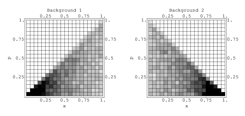
We define our cuts on variables $a$ and $b$ as:

$A$ and $B$ are true or false statements. If they are false the event is cut. With the cut points defined, we can then calculate the CSP for each event type: $P(A)$ or $P(B)$. In this toy model the CSPs can be calculated analytically because we know the underlying distributions. These values are shown in Table 2.

In the derivation of both the one and two background cases, we have assumed that the cuts $A$ and $B$ are uncorrelated. Of course, in real applications, it is unlikely to find two cuts which are perfectly uncorrelated. We would therefore like to find some general figure of merit to determine how correlation introduces errors into the background prediction. The following discussion will assume only one background source.

For a more realistic example, we discuss the use of this technique in the first search for the rare kaon decay $K_{L}\rightarrow\pi^{0}\pi^{0}\nu\bar{\nu}$ at E391a. E391a is dedicated experiment for the search for the rare kaon decay $K_{L}\rightarrow\pi^{0}\nu\bar{\nu}$ located at KEK. The experimental apparatus consists of a $4\pi$ hermetic photon veto system and an array of CsI, an inorganic crystal scintillator, for signal detection. The $K_{L}\rightarrow\pi^{0}\pi^{0}\nu\bar{\nu}$ decay has a Standard Model branching ratio of $(1.4\pm 0.4)\times 10^{-13}$ chiang. The bifurcation method is to predict the background to this mode from data.

The final state of $K_{L}\rightarrow\pi^{0}\pi^{0}\nu\bar{\nu}$ is four photons from the $\pi^{0}$’s and two unobservable $\nu$’s. Events are reconstructed by pairing the photons and calculating the $\pi^{0}$ decay vertices. The pairing with the smallest separation between $\pi^{0}$ vertices is selected. The signal region is defined in three kinematical variables: the transverse momentum of the $\pi^{0}$-$\pi^{0}$ system, the invariant mass of the the $\pi^{0}$-$\pi^{0}$ system, $M_{\pi^{0}\text{-}\pi^{0}}$, and reconstructed decay vertex, $Z$.

The signal region is selected to avoid the two primary background sources: $K_{L}\rightarrow\pi^{0}\pi^{0}\pi^{0}$ decays and neutron interactions with a membrane located downstream of the fiducial region. The $K_{L}\rightarrow\pi^{0}\pi^{0}\pi^{0}$ events have a mass peak below the $K_{L}$ mass and with relatively low $P_{T}$’s of under $100\text{MeV}/\text{c}$. Their decay vertices cover the full range of the fiducial decay region. The neutron related events are well separated in the decay vertex having a peak at the membrane position,  50 cm downstream of the fiducial region. The $K_{L}\rightarrow\pi^{0}\pi^{0}\nu\bar{\nu}$ signal box is defined as $100\text{MeV}/\text{c}<P_{T}<200\text{MeV}/\text{c}$, $268\text{MeV}/\text{c}^{2}<M_{\pi^{0}\text{-}\pi^{0}}<400\text{MeV}/\text{c}^{2}$, $300\text{cm}<Z<500\text{cm}$. The distribution of events in the $P_{T}~$-mass plane is shown in Fig. 8.

We divided our cuts into three groupings: the setup cuts, cut $A$ which contained most of the photon vetoes, and cut $B$ which contained primarily cuts on photon reconstruction quality in the CsI array. Using Eqn 7, we first tested the method on regions surrounding the signal box. We define a Low $P_{T}~$region with the same bounds on $M_{\pi^{0}\text{-}\pi^{0}}$ and $Z$ as the signal region and $P_{T}~$$<100\text{MeV}/\text{c}$. The High Mass Region is defined with the same bounds on $P_{T}~$and $Z$ as the signal region and $400\text{MeV}/\text{c}^{2}<M_{\pi^{0}\text{-}\pi^{0}}<500\text{MeV}/\text{c}^{2}$. The results of this are shown in Table 4. There is a significant discrepancy in the Low $P_{T}~$region, this is due to neglecting the correlation.

We estimated the cut correlation on the $K_{L}\rightarrow\pi^{0}\pi^{0}\pi^{0}$ background in its peak region using both data and Monte Carlo. The value of $\epsilon$ was found to be $(-.049\pm.035).$ We first apply Eqn 48 on the Low $P_{T}~$region and find a correction of $-6.67\pm 4.81$. This correction brings the prediction in Table 4 into much better agreement with data. We next apply Eqn 48 to the signal region and find a correction of $(-0.12\pm 0.12)$ events.

Low energy neutron interactions are difficult to simulate in general and we had the additional difficulty of not knowing the precise shape of the membrane in the beamline. Therefore, we used data to estimate the level of neutron background. The value of $N_{2}$ was estimated by fitting the distribution events in the High $P_{T}~$-High $Z$ region, $Z>500\text{cm}$ and $P_{T}>100\text{MeV}/\text{c}$. Events in this region are predominately core neutron events. We applied a set of loose cuts to ensure high statistics. We subtracted off the contribution of the $K_{L}\rightarrow\pi^{0}\pi^{0}\pi^{0}$ background using a Monte Carlo prediction of their contribution under the loose set of cuts. The fitted core neutron distribution was extended into the signal region and the total number core neutron events in the signal region was predicted from the distribution. Then the predicted number of events in the signal region were scaled down using the factor by which the population of events in the High $P_{T}~$-High $Z$ region were reduced. Using this procedure we estimate $N_{2}=2.16\pm 0.03_{\text{stat.}}\pm 1.05_{\text{syst.}}.$ The large systematic error comes from the subtraction of the $K_{L}\rightarrow\pi^{0}\pi^{0}\pi^{0}$ contribution in the High $P_{T}~$-High $Z$ region. The differences between the cut survival probabilities for core neutron events and $K_{L}\rightarrow\pi^{0}\pi^{0}\pi^{0}$ events were found by comparing the difference in cut effectiveness between the $K_{L}\rightarrow\pi^{0}\pi^{0}\pi^{0}$ peak in the Low Mass-Low $P_{T}~$region and the core neutron peak in the High Z region. The values which go into the correction and the computed correction are shown in Table 5.

The $K_{L}\rightarrow\pi^{0}\pi^{0}\pi^{0}$ decay has three ways in which it can cause backgrounds depending on the number of photons lost through veto inefficiency or fusion of photon clusters in the CsI. These three channels are not separated in the signal space, so our estimate of cut correlation includes contribution from these multiple background types.

The statistical uncertainties on both the correlation and the core neutron correction are large relative to their size. Therefore we decided to use these values as estimates of the systematic error made by neglecting the correlation and multiple background corrections. This results in a background prediction of $0.43\pm 0.32_{\text{stat.}}\pm 0.13_{\text{syst.}}$. Opening the signal box, we observed a single event, consistent with our background prediction.

The bifurcation analysis technique allows us to produce data driven background predictions while still maintaining a blind analysis. In this paper we have shown how to extend the bifurcation analysis to the case of two background sources and correlated cuts.

The correction for a second background source is effective for any level of secondary background. It does require information beyond which is available directly from a blind analysis. It requires a combination of Monte Carlo information about the relative strengths of the two backgrounds and how the cut survival probabilities vary between the two backgrounds. It also requires knowledge of $N_{0}$, the number of events in the signal box after the setup cuts.

Correlations between the two cuts cannot be handled as easily. Even when the correlation between cuts is linear, the effects on the background prediction are non-linear. Therefore, special care must be taken when selecting the cuts for the bifurcation analysis to avoid correlation.

One particular aspect of the impact of the prediction on the cut correlation is it’s dependance on the value of $N_{0}.$ This leads to two competing forces in optimizing the division of cuts into the setup cuts and the bifurcation cuts. From the perspective of minimizing statistical error in the bifurcation prediction, one would like a large value for $N_{0}$ with powerful cuts for cut $A$ and $B$, so that the statistical errors on the terms of Eqn 7 are small. On the other hand, a large $N_{0}$ means the prediction is sensitive to small correlations between the cuts.

References

- [1] S. Adler et al. “Evidence for the Decay ,” Phys. Rev. Lett. 79, 2204 (1997)
- [2] J. Nix et al. “First Search for ,” Phys. Rev. D 76, 011101(R) (2007)
- [3] Wolfram Research, Inc., Mathematica, Version 5.2, Champaign, IL (2005).
- [4] C.W. Chiang and F. J. Gilman. “ decays within and beyond the standard model,” Phys. Rev. D 62, 094026 (2000).