Spin measurements for 147Sm resonances: Further evidence for non-statistical effects
Abstract
We have determined the spins of resonances in the 147Sm() reaction by measuring multiplicities of -ray cascades following neutron capture. Using this technique, we were able to determine values for all but 14 of the 140 known resonances below keV, including 41 firm assignments for resonances whose spins previously were either unknown or tentative. These new spin assignments, together with previously determined resonance parameters, allowed us to extract level spacings ( and eV) and neutron strength functions ( and ) for and 4 resonances, respectively. Furthermore, cumulative numbers of resonances and cumulative reduced neutron widths as functions of resonance energy indicate that very few resonances of either spin have been missed below eV. This conclusion is strengthened by the facts that, over this energy range, Wigner distributions calculated using these values agree with the measured nearest-neighbor level spacings to within the experimental uncertainties, and that the values calculated from the data also agree with the expected values. Because a non-statistical effect recently was reported near eV from an analysis of 147Sm(n,) data, we divided the data into two regions; eV and eV. Using neutron widths from a previous measurement (corrected for new unresolved doublets identified in this work) and published techniques for correcting for missed resonances and for testing whether data are consistent with a Porter-Thomas distribution, we found that the distribution for resonances below 350 eV is consistent with the expected Porter-Thomas distribution. On the other hand, we found that data in the eV region are inconsistent with a Porter-Thomas distribution, but in good agreement with a distribution having We discuss possible explanations for these observed non-statistical effects and their possible relation to similar effects previously observed in other nuclides.
I Introduction
It recently has been shown Gl2000 that (n,) cross-section measurements can be very useful for improving calculated astrophysical rates for reactions involving particles. Furthermore, it has been shown Ko2004 that resonance analyses of such data can be even more useful in improving these rates. This is because a resonance analysis can eliminate confounding uncertainties and therefore allow more direct tests of parameters of nuclear models Ra2001; De2002; Ra2003a used to calculate these rates. However, to obtain the most useful information from a resonance analysis, it is necessary to know the spins of the resonances. This can be a problem because most of the nuclides for which (n,) cross sections are measurable at resonance energies have non-zero ground-state spins; hence, two spins are allowed even for low-energy s-wave resonances and it can be difficult or impossible to determine resonance spins using common techniques.
Information contained in the -ray cascades following neutron capture reactions can, in principle, sometimes be used to determine resonance spins. For example, in some cases it is expected that the average number of rays in the de-excitation cascades between the capturing states and the ground state will be different for the two s-wave spins. Consider the case of 147Sm. Because the ground-state spin of 147Sm is , s-wave neutrons lead to and resonances in 148Sm. In a very simple model in which only dipole transitions can occur, at least three -ray transitions are required to reach the ground state from a excited state whereas a minimum of four transitions are required in the case of a state. Hence, in this very simple model, resonances will have an average multiplicity of three and resonances an average multiplicity of four. In reality, the existence of other multipolarities will both broaden the multiplicity distributions as well as decrease the difference between average multiplicities for and resonances Co68; Co2004. Detector effects also can cause changes in the measured multiplicity distributions. However, as demonstrated in Ref. Ge93 the remaining difference in average multiplicity for the two spins still is measurable and independent of resonance energy and was used to determine spins of 91 147Sm resonances below 900 eV.
More recently Wa2003, an algorithm that combined Monte Carlo -ray cascades predicted by the nuclear statistical model with a Monte Carlo particle transport code was used to demonstrate that the predicted and measured multiplicity distributions for a multi-element NaI detector were in agreement for and resonances in 149Sm. A similar technique was used to demonstrate good agreement between the measured and predicted multiplicity spectra for a multi-element BaF2 detector Re2002.
The spin assignments from Ref. Ge93 were used in Ref.Ko2004 in an -matrix analysis of the data of Ref. Gl2000 to determine widths for 104 resonances below 700 eV. The resulting values revealed some surprises with respect to theoretical expectations. First, the -width distributions for both and resonances did not follow the expected distributions. In particular, the -width distributions were broader than reduced-neutron-width distributions instead of being intermediate to the distributions for neutrons and rays. Second, the ratio of strength functions for to resonances was less than one half of that predicted by theory. Furthermore, exploratory calculations were not able to find an nucleus potential that could reproduce the observed strength functions as well as the strength function ratio. Trying to reduce the strength function ratio to the observed value quickly led to strength functions which were orders of magnitude larger than measured. Most surprisingly, the data indicated that there is an abrupt decrease in the strength function ratio for energies above about 300 eV. Such an abrupt change cannot be reproduced with any optical model of strength functions.
As pointed out in Ref. Ko2004, the -width distributions as well as the striking decrease in the ratio near 300 eV depend on accurate spin assignments for the resonances, especially above 300 eV. Of the 104 resonances fitted in Ref. Ko2004, 23 resonances (5 below 300 eV) had tentative spin assignments. Therefore, we decided to make a new measurement of these resonance spins. It was expected that the new Detector for Advanced Neutron Capture Experiments (DANCE) at the Los Alamos Neutron Science Center (LANSCE) would make it possible to improve upon the measurement of Ref. Ge93 for several reasons. First, the flux at LANSCE is several orders of magnitude higher, allowing higher precision measurements even using smaller samples. Second, the DANCE detector has many more detector segments and a more sophisticated data acquisition system making more reliable multiplicity measurements possible. Third, the DANCE detector is made of BaF2 rather than NaI as used in Ref. Ge93. This change should lead to reduced backgrounds and improved timing.
II Experiment and data reduction
The experiment was performed using DANCE on flight path 14 at the Manuel Lujan, Jr. Neutron Scattering Center (MLNSC) at LANSCE Li90. DANCE is a 4 array of 160 BaF2 crystals positioned 20 m from the neutron production target. Details of the apparatus He2001; Re2004 and data acquisition Wo2006 have been published elsewhere, so only the salient features will be given herein.
Neutrons are generated at LANSCE via spallation reactions when an 800-MeV proton beam strikes a tungsten target. The average proton current on target was 110-120 A and the width of the proton pulses was 125 ns. Flight path 14 views one of the ambient-temperature water moderators at the MLNSC. The resulting neutron flux peaks near thermal energy and is approximately proportional to / over the range of our measurements.
The samples were placed inside an evacuated flight tube which was surrounded by a 6LiH neutron-scattering shield at the center of the DANCE array. Three samples of metallic samarium, which were enriched to 97.93% in 147Sm, 1 cm in diameter, and weighed 1.444, 3.208, and 10.410 mg, respectively were used. The samples were held in the neutron beam by attaching them to thin Al foils. Sample-out (blank Al backing foil) and neutron-scattering (C sample) background measurements also were made under the same conditions.
The neutron flux was monitored using three different sample/detector combinations downstream of the main sample position: i) a BF3 detector, ii) a fission chamber containing a 235U sample, and iii) solid state surface-barrier detectors which recorded tritons and particles from the 6Li(,)3H reaction occurring in a 6LiF sample.
Data were acquired as waveforms, using separate Acqiris transient digitizers for each detector, over a period of 200 to 250 s, triggered by a timing signal from the accelerator indicating the arrival of a proton pulse at the neutron production target. Three sets of runs, each with a different delay for this trigger, were required to cover the entire range from 10 s before each beam pulse from LANSCE to just below the lowest energy resonance at 3.397 eV. The waveforms were analyzed in real time to detect peaks. For each peak, a summary of the peak shape, together with a high resolution time stamp was written to a disk file. These data were sorted by a replay routine which generated information such as pulse-height (-ray energy), time-of-flight (neutron energy), and cluster multiplicity (number of rays detected) for each event. As explained in the references, cuts were applied to the data to reduce background from radioactive impurities in the BaF2 crystals. In addition, an overall pulse-height cut on the total -ray energy, MeV, was used to restrict events to those in the range expected from 147Sm(,) reactions. This stage of the analysis resulted in a two-dimensional spectrum, time-of-flight versus multiplicity, for each of the runs. The average fluxes recorded by the flux monitors were used to normalize sample-out runs for background subtraction. Fig. 1 shows representative sample-in, sample-out, and subtracted two-dimensional spectra.

Projections of the background subtracted spectrum onto the multiplicity axis for two time-of-flight regions corresponding to resonances having previous firm spin assignments are shown in Fig. 2.

These projections verify that there is a measurable, significant difference in the average multiplicity for the two different s-wave resonance spins. In principle, such projections at each time of flight (or over each resonance) could be used to determine the average multiplicities and hence the spins of the resonances as was done in Ref. Ge93. This is demonstrated in Fig. 3 where the average multiplicity as a function of neutron energy is plotted for four energy regions. For this figure, the average multiplicity is defined by:
| (1) |
where and are the multiplicity and (background-subtracted) total yield for that multiplicity, respectively, at neutron energy . Multiplicities one and greater than nine were not used because the statistical precision was too poor for these cases. As shown in the top two panels of Fig. 3, at low energies where most of the resonances are well resolved, average multiplicities fall into two bands at and for and , respectively. However, worsening resolution with increasing neutron energy limits the usefulness of this approach, and, as shown in the bottom two panels of Fig. 3, once the resonances are no longer adequately resolved from one another it becomes difficult or impossible to assign spins using this technique. The problem is that as instrumental resolution smears the peaks together, the multiplicity distribution at each neutron energy contains contributions from more than one resonance. If these resonances have different values, application of Eq. 1 will result in an value between the values for the two different spins. For example, the resonances at Su98 418.3, 625.3, and 651.9 eV all have values about midway between the expected values for and . In such cases, the average multiplicity often will display a positive or negative slope as a function of neutron energy and, if there is sufficient statistical precision and there are no other partially-resolved resonances nearby, it may be possible to discern that the peak in the yield curve actually is due to two resonances with different spins. For example, the peak near 65 eV was identified Ge93 as a doublet, with the lower-energy resonance having and the upper one , using this technique. On the other hand, although the versus curve displays a slope at the 418.3-, 625.3-, and 651.9-eV resonances, it was not possible to assign firm spins, or to determine if they were doublets, in any of these cases due to partially-resolved and resonances on either side. Another problem with using to assign spins is that, because it involves division by the background-subtracted counts, is very noisy between resonances and near very small resonances where there are few counts. For this reason, is plotted only near the peaks of the resonances in Fig. 3.
To overcome these difficulties, we employed a technique which effectively uses not only the average multiplicity but also the shapes of the distributions, and does not require division by the yield. This technique involves effectively subtracting the prototypical multiplicity distribution for () resonances from the multiplicity distribution at each neutron energy, thereby generating a curve as a function of neutron energy which peaks only at () resonances.
To understand how this technique works, consider that the total yield for a given multiplicity at neutron energy has, in general, contributions due to both and resonances;
| (2) |
Assuming that the average multiplicities as well as the shapes of the multiplicity distributions both remain constant for each of the two spins (which we have verified for isolated resonances in our data), it is possible to find a residual yield that will be zero for all resonances;
| (3) |
where and are integers, and is a normalization constant. For example, if and the distribution is symmetric, then Eq. 3 is satisfied for respectively, and . On the other hand, application of Eq. 3 to a resonance will yield a positive residual because is greater for resonances than it is for . These facts are graphically illustrated in Fig. 4. Furthermore, application of Eq. 3 to the data at energies where the yields contain contributions from both spins (i.e., Eq. 2) will recover the component:
| (4) | |||||
where, in the last step, Eq. 3 was used to eliminate the first two terms in the third line. Similarly, a second residual yield can be found that will be zero for all resonances;
| (5) |
Because was between and for both spins, the summation limits in Equations 3 and 5 were chosen so that one sum ended at while the second began at . Normalizations and were determined empirically to yield zero net counts in the vicinity of and resonances, respectively while yielding net positive counts for resonances of the other spin. The actual equations used are given in equations 6 and 7. Curves resulting from these equations are shown over the same energy regions as in Fig. 3, in Fig. 5, where the curve labeled was calculated according to:
| (6) |
Similarly, the curve labeled was calculated using the formula:
| (7) |


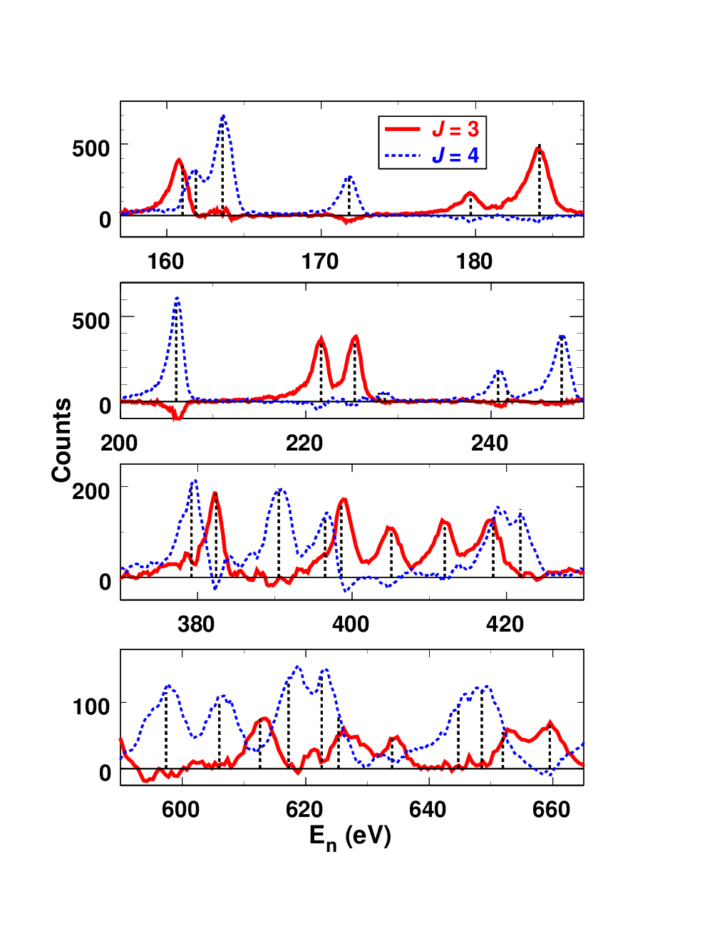

The overall normalization constant in Eq. 6 was chosen to yield peaks of approximately the same height from both equations so that the results could more easily be compared to one another on the same graph. Multiplicities one and greater than nine were not used because the statistical precision was too poor for these cases. The fact that the spin assignments for isolated resonances from this technique agree with those from using just the average multiplicities (both from this work as well as from Ref. Ge93) indicates that the multiplicity distributions do remain reasonably constant. The main advantage of this technique is that it makes spin assignments possible for several un- and partially-resolved resonances for which using failed. For example, as discussed above, it was not possible to make firm spin assignments for the 418.3-, 625.3-, and 651.9-eV resonances using . However, as shown in Fig. 5, the peak in the yield curve at 418.3 eV, which previously had been given a tentative assignment, is clearly due to two resonances with the lower-energy one having and the other . Fig. 6 depicts simulations based on this doublet in an attempt to further illustrate this new technique. In addition, Fig. 5 shows that the 625.3-, and 651.9-eV resonances have . There were many other similar cases. Overall, of the 140 resonances below keV, we were able to make firm assignments for 33 resonances with no previous assignments and eight firm assignments where previously there were only tentative assignments Su98.
Curves calculated using Equations 6 and 7 were used to assign the resonance values up to keV listed in Tables 1. We stopped at this energy because statistical analysis indicated that a significant fraction of resonances were beginning to be missed because of worsening resolution and statistical precision. Spins from previous measurements also are given in Table 1. Only 14 resonances below keV (nine below 700 eV) remain without firm assignments. Only six of our assignments disagree with those given in the compilation of Ref. Su98. Of these, our assignments for the partially-resolved doublet near 65 eV agree with those of the primary references Ge93; Al73a (indicating that perhaps an error was made in Ref. Su98 while compiling the data), another two involve other partially resolved doublets, and the final two previously were only tentative assignments. Finally, our data indicate that six previously known resonances (at 140.0, 290.1, 418.3, 513.5, 546.0, and 765 eV) actually are doublets. For all but the one at 140.0 eV, our data indicate that the two spin states are about equally strong, so we split the previously determined values equally between the two members of the doublet. Our data indicate that the component of the doublet at 140.0 eV is about twice as strong as the one, so we split the previous value by a ratio of 2:1.
| N | (eV) | |||||
| This Work | Ref. Su98 | Ref. Ge93 | Ref. Al73a | Ref. Po72 | ||
| 1 | 3.397 | 3 | 3 | 3 | 3 | |
| 2 | 18.36 | 4 | 4 | 4 | 4 | |
| 3 | 27.16 | 3 | 3 | 3 | 3 | 3 |
| 4 | 29.76 | 3 | 3 | 3 | 3 | 3 |
| 5 | 32.14 | 4 | 4 | 4 | 4 | |
| 6 | 39.70 | 4 | 4 | 4 | 4 | |
| 7 | 40.72 | 3 | 3 | 3 | 3 | 3 |
| 8 | 49.36 | 4 | 4 | 4 | (4) | |
| 9 | 58.09 | 3 | 3 | 3 | 3 | |
| 10 | 64.96 | 3 22 2 Partially resolved doublet. | (4) | 3 22 2 Partially resolved doublet. | 3 33 3 Unresolved doublet. | |
| 11 | 65.13 | 4 22 2 Partially resolved doublet. | (3) | 4 22 2 Partially resolved doublet. | 4 33 3 Unresolved doublet. | |
| 12 | 76.15 | 4 | 4 | 4 | 4 | |
| 13 | 79.89 | 4 | 4 | 4 | (4) | |
| 14 | 83.60 | 3 | 3 | 3 | 3 | 3 |
| 15 | 94.90 | 3 | ||||
| 16 | 99.54 | 4 | 4 | 4 | (4) | |
| 17 | 102.69 | 3 | 3 | 3 | 3 | (3) |
| 18 | 106.93 | 4 | 4 | 4 | (4) | |
| 19 | 108.58 | 4 | 4 | 4 | ||
| 20 | 123.71 | 3 | 3 | 3 | 3 | 3 |
| 21 | 140.00 | (3) 22 2 Partially resolved doublet. | 3 | 3 | 3 | |
| 22 | 140.10 | (4 ) 22 2 Partially resolved doublet. | ||||
| 23 | 143.27 | 4 | 4 | 4 | ||
| 24 | 151.54 | 3 | 3 | 3 | 3 | |
| 25 | 161.03 | 3 | 3 | 3 | 3 33 3 Unresolved doublet. | |
| 26 | 161.88 | 4 | 4 | 4 | 3 33 3 Unresolved doublet. | |
| 27 | 163.62 | 4 | 4 | 4 | (4) | |
| 28 | 171.80 | 4 | 4 | 4 | (4) | |
| 29 | 179.68 | 3 | 3 | 3 | ||
| 30 | 184.14 | 3 | 3 | 3 | 3 | 3 |
| 31 | 191.07 | 3 | 3 | 3 | ||
| 32 | 193.61 | 4 | 4 | 4 | ||
| 33 | 198.03 | 3 | 3 | 3 | ||
| 34 | 206.03 | 4 | 4 | 4 | (4) | |
| 35 | 221.65 | 3 | 3 | 3 | 3 33 3 Unresolved doublet. | |
| 36 | 225.28 | 3 | 3 | 3 | 3 33 3 Unresolved doublet. | |
| 37 | 227.9 | (4) | 433 3 Unresolved doublet. | |||
| 38 | 228.53 | 4 | 4 | 4 33 3 Unresolved doublet. | ||
| 39 | 240.76 | 4 | 4 | 4 | ||
| 40 | 247.62 | 4 | 4 | 4 | ||
| 41 | 257.13 | 3 22 2 Partially resolved doublet. | 3 | 3 33 3 Unresolved doublet. | ||
| 42 | 258.00 | 4 22 2 Partially resolved doublet. | 4 | 4 33 3 Unresolved doublet. | ||
| 43 | 263.57 | 3 | 3 | 3 | ||
| 44 | 266.26 | 4 | 4 | 4 | ||
| 45 | 270.72 | 3 | 3 | 3 | ||
| 46 | 274.40 | 3 | 3 | 3 | ||
| 47 | 283.28 | 4 | 4 | 4 | ||
| 48 | 290.10 | (4) 22 2 Partially resolved doublet. | (4) | (4) | ||
| 49 | 290.30 | (3) 22 2 Partially resolved doublet. | ||||
| 50 | 308.30 | 3 | 3 | 3 | ||
| 51 | 312.06 | 4 | 4 | 4 | ||
| 52 | 321.13 | 3 | 3 | 3 | ||
| 53 | 330.10 | 3 | 3 | 3 | ||
| 54 | 332.1 | 4 | 4 | 4 | ||
| 55 | 340.4 | 4 | 4 | 4 | ||
| 56 | 349.86 | 3 | 3 | 3 | ||
| 57 | 359.32 | 4 | 4 | 4 | ||
| 58 | 362.15 | 4 | 4 | 4 | ||
| 59 | 379.2 | 4 | 4 | 4 | ||
| 60 | 382.4 | 3 | 3 | 3 | ||
| 61 | 390.5 | 4 | 4 | 4 | ||
| 62 | 396.5 | 4 | (4) | (4) | ||
| 63 | 398.6 | 3 | 3 | 3 | ||
| 64 | 405.1 | 3 | 3 | 3 | ||
| 65 | 412.0 | 3 | 3 | 3 | ||
| 66 | 417.6 | 3 22 2 Partially resolved doublet. | (4) | (4) | ||
| 67 | 419.2 | 4 22 2 Partially resolved doublet. | ||||
| 68 | 421.8 | 4 | 4 | 4 | ||
| 69 | 433.1 | 4 | 3 33 3 Unresolved doublet. | |||
| 70 | 435.7 | 3 | 3 | 3 33 3 Unresolved doublet. | ||
| 71 | 440.2 | 4 | 4 | 4 | ||
| 72 | 446.9 | 3 | 3 | 3 | ||
| 73 | 458.6 | 4 | 4 | 4 | ||
| 74 | 462.9 | 3 | 3 | 3 | ||
| 75 | 476.0 | 4 | 4 | 4 | ||
| 76 | 479.8 | 3 | 3 | 3 | ||
| 77 | 486.4 | 3 | 3 | 3 | ||
| 78 | 496.2 | 4 | 4 | 4 | ||
| 79 | 498.6 | 3 | (3) | (3) | ||
| 80 | 513.5 | (3) 22 2 Partially resolved doublet. | 4 | 4 | ||
| 81 | 515.4 | (4) 22 2 Partially resolved doublet. | ||||
| 82 | 528.9 | 4 | 4 | 4 | ||
| 83 | 532.5 | 3 | 3 | 3 | ||
| 84 | 538.1 | 4 | 4 | 4 | ||
| 85 | 546.0 | (3) 22 2 Partially resolved doublet. | (3) | (3) | ||
| 86 | 546.2 | (4) 22 2 Partially resolved doublet. | ||||
| 87 | 553.2 | 3 | 3 | 3 | ||
| 88 | 554.5 | 4 | 4 | 4 | ||
| 89 | 559.7 | 3 | 3 | 3 | ||
| 90 | 563.4 | 4 | 4 | 4 | ||
| 91 | 567.6 | 3 | ||||
| 92 | 574.3 | 4 | 4 | 4 | ||
| 92 | 580.2 | 3 | 3 | 3 | ||
| 93 | 587.8 | 3 | 3 | 3 | ||
| 94 | 597.4 | 4 | 4 | 4 | ||
| 95 | 606.0 | 4 | 4 | 4 | ||
| 96 | 612.6 | 3 | ||||
| 97 | 617.2 | 4 | (3) | |||
| 98 | 622.6 | 4 | ||||
| 99 | 625.3 | 3 | ||||
| 100 | 634.0 | 3 | 3 | 3 | ||
| 101 | 644.7 | 4 | ||||
| 102 | 648.5 | 4 | ||||
| 103 | 651.9 | 3 | ||||
| 104 | 659.5 | 3 | (4) | (4) | ||
| 105 | 668.8 | 4 | 4 | 4 | ||
| 106 | 677.5 | 3 | ||||
| 107 | 683.1 | 4 | ||||
| 108 | 687.4 | 4 | ||||
| 109 | 697.0 | 4 | (4) | |||
| 110 | 702 | 3 | ||||
| 111 | 714.0 | 3 | 3 | 3 | ||
| 112 | 724 | 3 | ||||
| 113 | 729 | 4 | ||||
| 114 | 734 | 3 | ||||
| 115 | 744.3 | 4 | 4 | 4 | ||
| 116 | 754 | 4 | ||||
| 117 | 758 | 3 | ||||
| 118 | 764 | 4 22 2 Partially resolved doublet. | ||||
| 119 | 766 | 3 22 2 Partially resolved doublet. | ||||
| 120 | 796.2 | 3 | 3 | 3 | ||
| 121 | 808.0 | 4 | 4 | 4 | ||
| 122 | 821.0 | 4 | 4 | 4 | ||
| 123 | 836.1 | (4) | 4 | 4 | ||
| 124 | 847 | 4 | ||||
| 125 | 850 | (3) | ||||
| 126 | 854 | (4) | ||||
| 127 | 858 | 4 | ||||
| 128 | 864 | 3 | ||||
| 129 | 875.2 | 3 | 4 | 4 | ||
| 130 | 880 | 4 | ||||
| 131 | 896.1 | (4) | 4 | 4 | ||
| 132 | 911 | 3 | ||||
| 133 | 922 | 4 | ||||
| 134 | 930 | 3 | ||||
| 135 | 935 | 4 | ||||
| 136 | 943 | 4 | ||||
| 137 | 953 | (3) | ||||
| 138 | 962 | 3 | ||||
| 139 | 984 | 3 | ||||
| 140 | 991 | 4 | ||||
| 11footnotetext: Energies from Ref. Su98 except for some unresolved doublets. | ||||||
III Resonance parameter analysis and discussion
As a result of our new data, almost all the resonances below 700 eV have firm spin assignments. Therefore, it should be possible to perform a much better analysis of the resonance parameters than previously was possible.
III.1 Level spacings and neutron strength functions
Plots of the cumulative number of resonances as a function of resonance energy are shown in the top part of Fig. 7. Average level spacings can be calculated from the reciprocals of the slopes of these plots Mu81. These data indicate that a significant fraction of resonances are beginning to be missed for energies in excess of 700 eV. Therefore, only the data below this energy were used to determine the average level spacings. Dashed lines depict the results of linear fits to the data for 700 eV from which average level spacings of eV and eV for and resonances, respectively were determined. Uncertainties were calculated according to Ref. Mu81. The nearly equal level spacings for the two spin groups is in agreement with Fermi gas model predictions (see, for example Ref. Ki75).

Plotted in the bottom part of Fig. 7 are cumulative reduced neutron widths as functions of resonance energy. Neutron strength functions can be determined from the slopes of these plots Mu81. Neutron widths (except as noted above) were taken from Ref. Su98, which is based on Ref. Mi81. Because the measurement technique of Ref. Mi81 is expected to miss only resonances having very small neutron widths, and because such resonances contribute very little to the cumulative reduced neutron widths, the data over the entire region to 1 keV were used to determine the neutron strength functions. Dashed lines indicate the results of straight-line fits to the data from which strength functions and for and 4 resonances, respectively were determined. Uncertainties were calculated according to Ref. Mu81.
Further evidence that very few resonances have been missed below 700 eV is provided by the resonance spacing distributions. The integral nearest-neighboor spacing distributions for resonances below this energy are plotted in Fig. 8. We plotted integral rather than differential distributions for these data, as well as for the width distributions shown below, to avoid possible systematic effects due to the choice of binning widths. From these plots it can be seen that the measured spacings are in good agreement with the expected Wigner distributions Ly68. Furthermore, values Dy63 (which are sensitive measures of the expected longer range correlations in the level spacings) calculated from the data (0.40 for both spin states for resonances below 700 eV) are in excellent agreement with the expected values ( for both spin states). All these results indicate that there are very few missing or missasigned resonances for 700 eV.

III.2 Neutron width distributions
Reduced neutron widths for a single value are expected to follow a distribution with one degree of freedom () - the so-called Porter-Thomas (PT) distribution Po56. A distribution with degrees of freedom of widths has the form:
| (8) |
where is the probability, , is the average width, and is the gamma function for .
The PT distribution has been compared to reduced-neutron-width data in several instances (e.g., Refs. Po56; Ca76a; Ca94) and now is considered to be a well established fact. However, there are three main problems with such comparisons. First, the relatively small number of available resonances limits the statistical precision. Hence, these tests usually employ a statistical technique such as the maximum likelihood method to determine the value of the distribution from the data. Also, the formalism of error propagation was used in Ref. Ha84 to derive the standard deviation in the value determined from the data given the number of resonances used. Second, it is an unfortunate fact that the PT distribution is weighted towards small widths that are the most difficult to observe in experiments. Furthermore, the region of small widths is where the PT distribution differs most from the next closest distribution having . Therefore, tests of the PT distribution must include a consideration of missed resonances. For example, in Fig. 2 of Ref. Po56 several curves are given for different experimental sensitivities, to be used in determining the value from a set of measured reduced neutron widths. Third, care must be taken to avoid contamination from -wave resonances. Because neutron widths for -wave resonances are, on average, much smaller than for -wave ones, inclusion of only a small number of -wave resonances can lead to an erroneously small value being extracted from the distribution.
As a test case for the PT distribution, 147Sm has the advantages that a relatively large number of resonances are available and that the data should be free of -wave contamination. A minimum of 54 resonances were used in the tests described below, which is more than used in eight of the fourteen cases studied in Refs. Ca76a; Ca94. Furthermore, 147Sm is near both the maximum of the -wave as well as the minimum of the -wave neutron strength functions (). In addition, due to its relatively small average level spacing, a sufficient number of -wave resonances can be observed at relatively low energies, before the largest -wave neutron widths become comparable to the smallest -wave ones. In contrast, many of the nuclides studied in Ref. Ca94 are near the peak of the -wave strength function, having , and have level spacings 2.6 to 16 larger than 147Sm. Therefore, for these nuclides it was necessary to include resonances to much higher energies to obtain adequate sample sizes, and to use relatively high threshold values to avoid -wave contamination. Because theoretical distributions for different values differ most at small , using a higher threshold limits the sensitivity of the test.
Given the measured level spacing and strength function (which determine and the overall normalization) there are, in principle, no free parameters when comparing the measured reduced neutron widths to the expected PT distribution. Because we have determined level spacings and strength functions for both s-wave spin states, we can compare the distributions for each to the expected PT distributions as shown in Fig. 9. As can be seen in this figure, there appears to be substantial disagreement between the data and the expected distributions. To quantify these differences, we used the values together with Eq. 2 and Fig. 2 of Ref. Po56 (which are based on the maximum likelihood method) to estimate values. For and 4, the first term on the left hand side of Eq. 2 (, where the sum runs from to , the number of resonances) in Ref. Po56 equals and , respectively. To use these values with Fig. 2 of this reference, it is necessary to choose a threshold value for the experiment, , which is the antilog of the value of at which the overall efficiency of detecting a reduced neutron width this small is . According to Ref. Po56, the most probable value is , so we used the curve for this value to obtain and for and 4, respectively. The uncertainties were calculated according to Eq. 2.14 in Ref. Ha84 from which it can be concluded that the distributions for and 4 are 4.5 and 2.3 standard deviations different from the expected value of for a PT distribution.

Other methods have been devised to correct for missed resonances, and other statistical tests may be used to ascertain if the data are consistent with a PT distribution. Before proceeding further however, first let us consider the fact that a non-statistical effect recently was reported Ko2004 near eV from an analysis of data. With this in mind, we divided the data into two groups from eV and eV. Also, because our analysis indicates that the average reduced neutron widths are equal for and 4, we combined the data (as ) for the two spins to increase the statistical precision. In Ref. Mi81, the data were combined as (where where the spin of the target nuclide 147Sm) as typically is done when the resonance spins are unknown. However, combining two spin groups in this way implicitly assumes that the number of resonances are proportional to , which we have shown is not the case. Neutron width distributions for the two energy regions are shown in Fig. 10. From this figure, it appears that the distribution changes shape between the two energy regions. Below 350 eV, the shape appears to be very well described by a PT distribution. Using Eq. 2 and (the curve in) Fig. 2 in Ref. Po56, leads to for the lower-energy region, in excellent agreement with PT. In contrast, this same method leads to for the eV region, or more than 11 standard deviations different from . To obtain this result, we used the equations in Ref. Po56 to extend the curves in Fig. 2 of that reference (which ends at ). For such large values, curves for the different values are nearly the same. One problem with the technique of Ref. Po56 is that the correction for missed resonances is made using an energy-independent threshold value , whereas in most experiments the sensitivity decreases with increasing energy. Therefore, it seems prudent to employ a more realistic correction for the number of missed resonances.

In Ref. Fu65, a technique for calculating the number of missed resonances was devised which is based on realistic experimental conditions. The technique as it is laid out in Ref. Fu65 also assumes the reduced neutron widths obey a PT distribution. We have shown above that the neutron widths for resonances below 350 eV are in good agreement with PT. Therefore, we applied the technique of Ref. Fu65 to the data in this region to obtain corrected and values (and hence corrected values for the number of resonances in the 350-eV interval and corrected values for the average reduced neutron width) and assumed these values remain the same for the next 350-eV interval.
To apply this technique, it is necessary to determine an energy-dependent threshold below which resonances are missed, , where and are constants determined from the data and type of experiment, respectively. Ref. Fu65 indicates that for the present experiments and, as can be seen in Fig. 11, this choice of seems to agree well with the experimental threshold across a wide energy range. An examination of the reduced neutron widths below 350 eV indicates that the most sensitive limit is set by the 228.53-eV resonance, from which is obtained. Following the iterative procedure of Ref. Fu65, these values of and lead to a corrected average level spacing of eV (for both spins combined, with uncertainty calculated according to Ref. Mu81) and negligible change to . Assuming the relative number of resonances for the two different spins remains unchanged, the corrected spin-separated average level spacings are eV and eV. Hence, this technique indicates that 5 resonances were missed by 350 eV, or . Peaks in our data due to small amounts of 149,150Sm (0.50 and 0.17 at%, respectively) in the sample indicate that this is a conservative estimate and that the actual number of missed resonances is smaller. Of the observed 149,150Sm resonances, the one at 68.3 eV yields the most sensitive limit. Using this resonance, the parameters in Ref. Su98, the assayed amount of 149Sm in the sample, and the methods of Ref. Fu65 yields by 350 eV. Reduced neutron widths for 147Sm and effective values for 149,150Sm are shown together with the and threshold curves in Fig. 11.

In addition to providing corrections for the number of missed resonances, the calculations above also make it possible to do a more careful and realistic maximum likelihood analysis as described in Ref. Ca94. Instead of the somewhat arbitrary threshold used in Ref. Po56, in the technique of Ref. Ca94, an energy-independent threshold is determined from the data by examining a plot such as Fig. 11. The threshold value is chosen such that, within the energy range being considered, all s-wave resonances appear to have been observed and all p-wave resonances excluded. As explained above, the latter consideration can be neglected in the present case. From Fig. 11, it can be seen that the conservative () threshold curve implies that meV is a reasonable threshold value for eV. Similarly, meV is a reasonable threshold value for eV. With these threshold choices, applying the technique of Ref. Ca94 leads to for the eV region, and for the eV region. Hence, this improved analysis leads to the same conclusion as applying the method of Ref. Po56: The data in the lower energy region are consistent with a PT distribution, but the higher-energy data are inconsistent with PT. Even if the very conservative threshold of meV is assumed for the eV region, the value obtained () still is inconsistent with a PT distribution at the level. Uncertainties were dominated by finite sampling errors, which were determined in the usual way when maximum likelihood estimators are used, as described in Ref. Ca94. These uncertainties tend to be substantially larger than those calculated following Ref. Ha84, which is based on the formalism of error propagation.
As a further check, a second statistical technique was applied. The Kolmogorov-Smirnov (KS) test Co80 can be used to test the hypothesis that theoretical and measured distributions are equivalent. This test involves calculating the maximum vertical distance between the data and the hypothesized distribution and accounts for the fact that a limited number of samples were measured in the experiment. The expected PT distribution using the more conservative correction for missed resonances () is shown in Fig. 10. It appears to be in excellent agreement with the data for eV and significantly different from the data for eV. We applied the KS test to the data in both energy regions. Using , we calculated and for the eV and eV regions, respectively. These values together with the number of observed resonances were used to calculate values of and for the eV and eV regions, respectively. These values indicate the hypothesis that the data are consistent with a PT distribution is accepted for the lower energy region, but rejected at the confidence level for the eV region. KS tests of these same data compared to a distribution with 3.5 degrees of freedom result in the opposite conclusion; the hypothesis that the data are consistent with this distribution is accepted for the higher energy region (), but rejected at the confidence level for the eV region. Although the data in the eV region are in better agreement with larger values, intermediate degrees of freedom (e.g., and , for ) cannot be excluded. Taken together, both the maximum likelihood and KS methods indicate the shape of the distribution changes from PT to at eV. Results from KS tests of the various distributions are summarized in Table 2.
In doing the above tests, we have calculated the correction for missed resonances using the data in the eV region, and assumed the same number of resonances () in the eV region. Although it could be argued that it might be better to use the data in the eV region to obtain the corrected number of resonances in this region, there are at least three reasons why our approach is better. First, as shown in Fig. 11, sensitivity to small resonances is greatest at lower energies. Hence by using the data in the eV region, the correction factor is, in principle, smaller and any unknown systematic errors should be less important. Second, all such correction methods must assume a neutron-width distribution. As discussed above, applying statistical tests to the data in the eV region indicate that these data are in good agreement with a PT distribution. Hence, it should be safe to apply the method of Ref. Fu65 (which assume a PT distribution) to the data in this region to obtain the corrected number of resonances. On the other hand, these same statistical tests indicate that the data in the eV region do not follow a PT distribution, so it may not be valid to apply the technique of Ref. Fu65 to obtain the corrected number of resonances in this region from these data; furthermore, to do so would result in a somewhat circular test (i.e., assuming to obtain the corrected number of resonances with which to test if ). Third, all such correction techniques are multiplicative in nature; they obtain the corrected number of resonances by multiplying the observed number of resonances by a correction factor Therefore, a significant systematic error can result if the wrong neutron-width distribution is assumed. This is because there are fewer resonances having small neutron widths for a distribution than for a PT one. Therefore, for a given threshold such as shown in Fig. 11, fewer resonance will be missed for a distribution than for a PT one. Hence, if a PT distribution is assumed, but the distribution actually has , the resultant corrected number of resonances will be too large. To illustrate this point, we adapted the technique of Ref. Fu65 to a distribution. Applying the technique of Ref. Fu65 (with ) to the data in the eV region, assuming results in a corrected average level spacing of eV, which is standard deviations Mu81 different from the corrected value ( eV) in the eV region. In contrast, applying this same technique to these same data, but assuming results in a corrected average level spacing of eV (), only 1.2 standard deviations from the result obtained for the eV region. Hence, these calculations indicate the approach we have taken is reasonable, and further indicate that the data in the eV region are inconsistent with a PT distribution.
As a further check on the correction for missed resonances, we applied the technique of Ref. Ge81, which is based on the statistic. The present case is very similar to the 235U example discussed in Ref. Ge81, from which it can be calculated that most likely 147Sm+ resonances were missed for each spin state for eV. Hence, the corrected number of resonances for eV from this technique is smaller than, but consistent with, the value obtained above following the technique of Ref. Fu65.
One problem with using the KS test is that it is nonparametric, but we have determined parameters of the theoretical distribution from the data. In such cases, Ref. Co80 indicates that the KS test is conservative, and Refs. Co80; Li67 describe how to modify the KS test to make it parametric: The test statistic remains unchanged, but different tables of critical values are used, and these values are calculated using Monte Carlo techniques.
It is straightforward to adapt the KS test when is determined from the data. We wrote a computer program which drew (where in the present case because this was the number of observed resonances in the -eV region) random values from a PT distribution. The average reduced neutron width for this sampled set then was calculated, and the maximum vertical difference (the statistic) between a PT distribution with this and the random samples was calculated. The program performed this task 30000 times to construct a distribution of values. As a check of the program, a second set of values was obtained in the standard KS sense (without calculating from the sampled data). The values calculated using these standard values were found to agree with those in references (e.g., Ref. Co80). Furthermore, it was found that there were fewer large values of the statistic when was determined from the sampled data compared to the standard KS values, verifying that the KS test is conservative. For example, in the present case for a PT distribution having , the value calculated from the data was 0.2432 (in the -eV region), and the value increased from for the KS test to for this parametric variation.
Adapting the KS test to the case where also is determined from the data requires additional assumptions. We assumed that the resonances were spaced according to a Wigner distribution and that the method of Ref. Fu65 can be used to correct for missed resonances. Hence, for the -eV region, we assumed a starting value of eV (), and randomly sampled level spacings from this Wigner distribution to obtain resonance energies between and eV. We then used random sampling to obtain a set of reduced neutron widths from a PT distribution. We then applied the same threshold curve determined from the data to remove those values which were below threshold, resulting in resonances with averaged reduced neutron width . Subsequently, the method of Ref. Fu65 was used to obtain corrected and values. The PT distribution with these corrected parameters was compared to the sampled data to obtain the value for this sample. Reduced neutron widths below the maximum threshold for the correction technique of Ref. Fu65 were excluded from this calculation. This procedure was repeated 30000 times to construct the distribution of values. These calculations revealed that when both and are determined from the data, there are even fewer large values than in either the standard KS case or the case where alone is determined from the data. For example, if a PT distribution having is compared to the data in the -eV region, is obtained, for which the standard KS test yields . In contrast, this second modified KS test yields in this case.
In addition to demonstrating that the data in the -eV region are inconsistent with a PT distribution to high confidence, the above tests also illustrate that this conclusion is unaltered by assuming, within reason, a higher threshold value or more missing resonances (than applying the method of Ref. Fu65 to the data for eV yields). For example, the final version of the ”parametric” KS test described above assumes that 10 more resonances were missed (17 versus 7) in the -eV region.
III.3 Discussion
We have employed the same published techniques that have been used to demonstrate the validity of the PT distribution for reduced neutron widths to show that the PT distribution is inconsistent with the current data for eV to high confidence. This conclusion is in contrast with Ref. Ko2004 where it was found that the reduced neutron width distributions agreed fairly well with PT distributions. However, our new DANCE data show that many of the spin assignments used in Ref. Ko2004 as well as the relative number of to resonances assumed (according to ) in that reference were incorrect.
Similar deviations from a PT distribution have been reported for 232Th Ri69; Fo71; Fo71a; Ra72, as well as for five odd-A nuclides (151Sm, 163Dy, 167Er, 175Lu, and 177Hf) Ca76a for which the statistic indicated that very few resonances had been missed.
It is interesting to note that the reduced-neutron-width distribution for 232Th changes shape in a manner similar to what we have found for 147Sm; from having for one energy range ( eV) Ri69; Fo71; Fo71a; Ra72, to being consistent with PT for another energy range ( eV) Ra72; Ca94. It also is interesting to note that the deviation from a PT distribution for 147Sm occurs at the same energy where an anomaly in the strength function ratio has been reported Ko2004. Finally, it may be noteworthy that all seven of the reported deviations from PT discussed above are limited to relatively low energies, eV and nuclides in which deformation may be important. Perhaps all these effects can be explained by the same theory.
In the early days of neutron width measurements, an exponential distribution () seemed to be favored Hu55 for the reduced neutron widths. Subsequently it was shown Po56, however, that a PT distribution fitted the data better. In addition to fitting the data better, plausible arguments were put forward to explain why the underlying physics should lead to a PT distribution. The assumptions that expansion coefficients of the compound nuclear wave function follow a Gaussian distribution with zero mean, that these coefficients are real (because, due to time-reversal invariance, the reduced width amplitudes have been shown to be real Wi47), and that neutron scattering is a single-channel process at these energies, leads to the PT distribution Ly68. Consequently, if one or more of these conditions does not hold the result may be a width distribution different from PT.
For example, the existence of additional channels results in values greater than one. It is well known, for example, that the distribution of total radiation widths following neutron capture is described by a distribution with many degrees of freedom by virtue of the many different possible -ray channels from the capturing state. However, the lowest-lying excited state of 147Sm is at keV. So, there are no known neutron channels in addition to the elastic one in the energy range of our analysis. Furthermore, the technique used (transmission measurement) should yield neutron widths that are fairly insensitive to inelastic channels.
Another way of adding an additional effective channel might be through a non-statistical nuclear structure effect such as a doorway state. It is interesting that a (parity) doorway model has been proposed to explain the so-called sign effect St98 in parity-violating asymmetries for p-wave 232Th+n resonances, which occurs at about the same energy as the reported Ri69; Fo71; Fo71a; Ra72 deviation from a PT distribution for the neutron widths in this nuclide. It was expected (based on arguments similar to those leading to the PT distribution) that the signs of these parity-violating asymmetries would be random. However, all ten measured asymmetries for resonances below 250 eV had the same sign. Models proposed to explain this sign effect are based on either distant Bo92; Au92; Au92a; Fl92; Ko92; Ca93a; Ca95; Le92; Au94 or nearby Au95; Fl95; Au96; De96; Hu95; Fe96; Lo96 (parity) doorway states. Perhaps the same type of model could be invoked to explain the observed deviations in the neutron width distributions from the expected PT shape, while at the same time these deviations might provide some clue to the physical origins of the doorway. The doorway might produce deviations from the PT shape by effectively providing a second channel. In addition, it is interesting to note the local-doorway model of Ref. Au95a is associated with the known octupole deformation of 233Th. Deformation also is known to be significant in the 148Sm region Ah93, and because deformation could have a large effect on decay, it is possible that the same type of model might also explain the strange behavior of the strength function ratio Ko2004. There are at least two arguments against a doorway explanation for the observed effects in 147Sm+n resonances as well as the observed deviation of the 232Th+n neutron-width distribution from the expected PT distribution. First, the observed effects are much narrower than expected for a doorway state. Second, doorways having such large effects on the neutron-width distributions presumably also should be visible (as large steps) in strength-function plots such as those shown in the bottom part of Fig. 7. However, there are no such effects visible in this figure nor in the corresponding plot for 232Th+n Ra72.
Deviations from a PT distribution also may be caused by forms of symmetry breaking. For example, isospin-symmetry breaking has been put forward Hu2000 as an explanation for differences between reduced-width data and a PT distribution. However, the distributions resulting from these kinds of symmetry breaking are expected to be superpositions of two PT distributions rather than a distribution with as observed herein.
Other forms of symmetry breaking can lead to width distributions having . For example, time-reversal invariance violation (TRIV) implies compound nuclear expansion coefficients that are complex, and hence a second degree of freedom and therefore a distribution having for the neutron widths. This extra degree of freedom also should effect the level-spacing distribution Gu98, leading to fewer small spacings than a Wigner distribution. Unfortunately, these effects in the level-spacing distribution appear to be too small to observe in the present case. Spacing distributions for both and for the two different energy regions are shown in Fig. 12. Also shown are the expected spacing distributions corresponding to PT (Wigner distribution, or Gaussian Orthogonal Ensemble, GOE) and (the so-called Gaussian Unitary Ensemble, GUE) distributions for the reduced neutron widths. There is no significant difference between the two measured distributions for and the data are consistent with either theoretical distribution. Although there is some difference between the measured distributions for the two energy regions in the case, given the small number of resonances in each region, this difference cannot be used to rule out either theoretical distribution at a reasonable confidence level. Results from KS tests of the various distributions are summarized in Table 2.
| Quantity | Distribution | (eV) | (%) | |||
|---|---|---|---|---|---|---|
| PT | 3+4 | 0-350 | 0.0919 | 56 | 63.40 | |
| with | 3+4 | 0-350 | 0.2435 | 56 | 99.90 | |
| with | 3+4 | 0-350 | 0.4075 | 56 | 100.00 | |
| PT | 3+4 | 350-700 | 0.2432 | 54 | 99.87 | |
| with | 3+4 | 350-700 | 0.1167 | 54 | 78.72 | |
| with | 3+4 | 350-700 | 0.0667 | 54 | 40.75 | |
| GOE | 3 | 0-350 | 0.1261 | 27 | 60.89 | |
| GUE | 3 | 0-350 | 0.1753 | 27 | 83.04 | |
| GOE | 4 | 0-350 | 0.1522 | 27 | 70.04 | |
| GUE | 4 | 0-350 | 0.2166 | 27 | 93.18 | |
| GOE | 3 | 350-700 | 0.1944 | 24 | 85.67 | |
| GUE | 3 | 350-700 | 0.2224 | 24 | 92.02 | |
| GOE | 4 | 350-700 | 0.1122 | 28 | 53.98 | |
| GUE | 4 | 350-700 | 0.1548 | 28 | 76.35 | |
| GOE | 3+4 | 0-350 | 0.0996 | 55 | 68.52 | |
| GUE | 3+4 | 0-350 | 0.0920 | 55 | 62.86 | |
| GOE | 3+4 | 350-700 | 0.1107 | 53 | 74.61 | |
| GUE | 3+4 | 350-700 | 0.0922 | 53 | 61.73 |

Data for the two spins can be combined to increase the statistical precision. However, combining the two spins also decreases the difference between the two theoretical distributions. The net effect is that combining the two spins does not improve the ability to distinguish between the two theoretical distributions. This is shown in Fig. 13 where spacing distributions for the two spins combined are shown for the two energy regions and compared to the two theoretical distributions. Although there appears to be a difference in shape between the data in the two regions, neither data set can be used to rule out either theoretical distribution at the 95% confidence level. Curiously, the level-spacing data in the upper energy region for the two spins combined looks very similar to a Wigner distribution for a single spin.

IV Summary and Conclusions
We have used information contained in multiplicity distributions of rays following neutron capture to assign spins of 147Sm resonances. We have shown that the DANCE detector at LANSCE is an excellent apparatus for this application. We have devised a new technique for using the measured multiplicity information to discern resonance spins. We have demonstrated that this new technique is superior to using the average multiplicity for assigning spins to closely-spaced resonances. Spins were determined for 33 resonances without previous assignments and 8 firm spin assignments were made for resonances previously having only tentative assignments. There are several other nuclides for which this technique should be applicable and so future measurements of this type could lead to a wealth of new resonance parameter data.
We used these new spin assignments together with reported Mi81; Su98 neutron widths to determine average level spacings, neutron strength functions, and level-spacing and reduced-neutron-width distributions for and 4 resonances separately. Our analysis shows that there are very few missing resonances below eV. Furthermore, using the same techniques that have been used to correct for missed resonances and to demonstrate the validity of the PT distribution for reduced neutron widths, we have shown that the present data are inconsistent with PT. Specifically, the reduced neutron width distribution changes shape near eV, from being consistent with PT below this energy to being inconsistent with PT for the next 350 eV. This change occurs at the same energy as a previously reported Ko2004 anomaly in the strength-function ratio for resonances. A similar unexplained deviation from PT was reported for neutron resonances in 232Th Ri69; Fo71; Fo71a; Ra72 and five odd-A nuclides Ca76 at about the same energy. We have discussed several possible explanations for these observed non-statistical effects. Of the considered explanations (a previously-unknown low-lying excited state in 147Sm, a doorway state, and TRIV) only TRIV is consistent with, but by no means proved by, the data. Indeed we know of no physical explanation why TRIV would be manifested in these nuclides at this energy at such levels. It seems more likely that an unknown nuclear structure effect, perhaps one related to deformation, is responsible for the reported anomalies Ko2004; Ri69; Fo71; Fo71a; Ra72. Finally, with current techniques it should be possible to significantly improve both the accuracy and sensitivity of the previous experiment on which the present 147Sm neutron widths are based Mi81. Therefore, it could be worthwhile to make new high resolution and high sensitivity neutron capture and total cross section measurements on 147Sm.
Acknowledgements.
We would like to thank J. D. Bowman, J. A. Harvey, G. E. Mitchell, and T. F. Papenbrock for fruitful discussions, and the Referees for helpful suggestions. This work was supported in part by the U.S. Department of Energy under Contract No. DE-AC05-00OR22725 with UT-Battelle, LLC. This work has benefited from the use of the LANSCE facility at Los Alamos National Laboratory which was funded by the U.S. Department of Energy and operated by the University of California under Contract W-7405-ENG-36.References
- (1) Y. M. Gledenov, P. E. Koehler, J. Andrzejewski, K. H. Guber, and T. Rauscher, Phys. Rev. C 62, 042801(R) (2000).
- (2) P. E. Koehler, Y. M. Gledenov, T. Rauscher, and C. Frōhlich, Phys. Rev. C 69, 015803 (2004).
- (3) T. Rauscher and F.-K. Thielemann, Atomic Data Nucl. Data Tables 79, 47 (2001).
- (4) P. Demetriou, C. Grama, and S. Goriely, Nucl. Phys. A707, 253 (2002).
- (5) T. Rauscher, Nucl. Phys. A719, 73c (2003).
- (6) C. Coceva, F. Corvi, P. Giacobbe, and C. Carraro, Nucl. Phys. A117, 586 (1968).
- (7) F. Corvi and M. Przytula, Physics of Particles and Nuclei 35, 767 (2004).
- (8) G. Georgiev, Y. S. Zamyatnin, L. B. Pikelner, G. V. Muradian, Y. V. Grigoriev, T. Madjarski, and N. Janeva, Nucl. Phys. A565, 643 (1993).
- (9) S. Wang, M. Lubert, Y. Danon, N. C. Francis, R. C. Block, F. Bečvář, and M. Krtička, Nucl. Instru. Methods Phys. Res. A 513, 585 (2003).
- (10) R. Reifarth, M. Heil, F. Kāppeler, F. Voss, K. Wisshak, F. Bečvář, M. Krtička, R. Gallino, and Y. Nagai, Phys. Rev. C 66, 064603 (2002).
- (11) P. W. Lisowski, C. D. Bowman, G. J. Russell, and S. A. Wender, Nucl. Sci. Eng. 106, 208 (1990).
- (12) M. Heil, R. Reifarth, M. M. Fowler, R. C. Haight, F. Kāppeler, R. S. Rundberg, E. H. Seabury, J. L. Ullmann, J. B. Wilhelmy, and K. Wisshak, Nucl. Instrum. Methods Phys. Res. A 459, 229 (2001).
- (13) R. Reifarth, T. A. Bredeweg, A. Alpizar-Vicente, J. C. Browne, E.-I. Esch, U. Greife, R. C. Haight, R. Hatarik, A. Kronenberg, J. M. O’Donnell, R. S. Rundberg, J. L. Ullmann, D. J. Vieira, J. B. Wilhelmy, and J. M. Wouters, Nucl. Instrum. Methods in Phys. Res. A 531, 530 (2004).
- (14) J. M. Wouters, A. A. Vicente, T. A. Bredeweg, E.-I. Esch, R. C. Haight, R. Hatarik, J. M. O’Donnell, R. Reifarth, R. S. Rundberg, J. M. Schwantes, S. A. Sheets, J. L. Ullmann, D. J. Vieira, and J. B. Wihelmy, IEEE Trans. Nucl. Sci. 53, 880 (2006).
- (15) S. I. Sukhoruchkin, Z. N. Soroko, and V. V. Deriglazov, Low Energy Neutron Physics (Springer-Verlag, Berlin, 1998).
- (16) L. Aldea, F. Bečvář, H. T. Hiep, S. Pospisil, S. A. Telezhnikov, and V. G. Tishin, Technical Report No. B-3-7390, Joint Institute for Nuclear Research, Dubna, Russia (unpublished).
- (17) Y. P. Popov, M. Przytula, R. F. Rumi, M. Stempinski, and M. Frontasyeva, Nucl. Phys. A188, 212 (1972).
- (18) S. F. Mughabghab, M. Divadeenam, and N. E. Holden, Neutron Cross Sections (Academic, New York, 1981), Vol. 1.
- (19) G. J. Kirouac and H. M. Eiland, Phys. Rev. C 11, 895 (1975).
- (20) M. Mizumoto, Nucl. Phys. A357, 90 (1981).
- (21) J. E. Lynn, The Theory of Neutron Resonance Reactions (Oxford University, Oxford, 1968).
- (22) F. J. Dyson and M. L. Metha, J. Math. Phys. 4, 701 (1963).
- (23) C. E. Porter and R. G. Thomas, Phys. Rev. 104, 483 (1956).
- (24) H. A. Camarda, Phys. Rev. C 13, 2524 (1976).
- (25) H. S. Camarda, Phys. Rev. C 49, 1391 (1994).
- (26) H. L. Harney, Z. Phys. A 316, 177 (1984).
- (27) T. Fuketa and J. A. Harvey, Nucl. Instrum. Methods 33, 107 (1965).
- (28) W. J. Conover, Practical Nonparametric Statistics (John Wiley and Sons, New York, 1980).
- (29) P. D. Georgopulos and H. S. Camarda, Phys. Rev. C 24, 420 (1981).
- (30) H. W. Lilliefors, Journal of the American Statistical Association 62, 333 (1967).
- (31) P. Ribon, Ph.D. thesis, Universite de Paris, 1969.
- (32) L. Forman, A. D. Schelberg, J. H. Warren, M. V. Harlow, H. A. Grench, and N. W. Glass, in Proceedings of the Third Conference on Neutron Cross Sections and Technology, edited by J. A. Harvey and R. L. Macklin (National Technical Information Service, U. S. Dept. of Commerce, Springfield, Virginia, 1971), p. 735.
- (33) L. Forman, A. D. Schelberg, J. H. Warren, and N. W. Glass, Phys. Rev. Lett. 27, 117 (1971).
- (34) F. Rahn, H. S. Camarda, G. Hacken, J. W. W. Havens, H. I. Liou, J. Rainwater, M. Slagowitz, and S. Wynchank, Phys. Rev. C 6, 1854 (1972).
- (35) D. J. Hughes and J. A. Harvey, Phys. Rev. 99, 1032 (1955).
- (36) E. P. Wigner and L. Eisenbud, Phys. Rev. 71, 29 (1947).
- (37) S. L. Stephenson, J. D. Bowman, B. E. Crawford, P. P. J. Delheij, C. M. Frankle, M. Iinuma, J. N. Knudson, L. Y. Lowie, A. Masaike, Y. Matsuda, G. E. Mitchell, S. I. Penttila, H. Postma, N. R. Roberson, S. J. Seestrom, E. I. Sharapov, Y.-F. Yen, and V. W. Yuan, Phys. Rev. C 58, 1236 (1998).
- (38) J. D. Bowman, G. T. Garvey, C. R. Gould, A. C. Hayes, and M. B. Johnson, Phys. Rev. Lett. 68, 780 (1992).
- (39) N. Auerbach, Phys. Rev. C 45, R514 (1992).
- (40) N. Auerbach and J. D. Bowman, Phys. Rev. C 46, 2582 (1992).
- (41) V. V. Flambaum, Phys. Rev. C 45, 437 (1992).
- (42) S. E. Koonin, C. W. Johnson, and P. Vogel, Phys. Rev. Lett. 69, 1163 (1992).
- (43) B. V. Carlson and M. S. Hussein, Phys. Rev. C 47, 376 (1993).
- (44) B. V. Carlson, M. S. Hussein, A. K. Kerman, and C.-Y. Lin, Phys. Rev. C 52, R11 (1995).
- (45) C. H. Lewenkopf and H. A. Weidenmuller, Phys. Rev. C 46, 2601 (1992).
- (46) N. Auerbach and V. Spevak, Phys. Rev. C 50, 1456 (1994).
- (47) G. Audi and A. H. Wapstra, Nucl. Phys. A595, 409 (1995).
- (48) V. V. Flambaum and B. G. Zelevinsky, Phys. Lett. B 350, 8 (1995).
- (49) N. Auerbach, V. V. Flambaum, and V. Spevak, Phys. Rev. Lett. 76, 4316 (1996).
- (50) B. Desplanques and S. Noguera, Nucl. Phys. A598, 139 (1996).
- (51) M. S. Hussein, A. K. Kerman, and C.-Y. Li, Z. Phys. A 351, 301 (1995).
- (52) H. Feshbach, M. S. Hussein, and A. K. Kerman, in Parity and Time Reversal Violation in Compound Nuclear States and Related Topics, edited by N. Auerbach and J. D. Bowman (World Scientific, Singapore, 1996), p. 157.
- (53) L. Y. Lowie, Ph.D. thesis, North Carolina State University, 1996.
- (54) N. Auerbach, J. D. Bowman, and V. Spevak, Phys. Rev. Lett. 74, 2638 (1995).
- (55) I. Ahmad and P. A. Butler, Annu. Rev. Nucl. Part. Sci. 43, 71 (1993).
- (56) H. S. Hussein and M. P. Pato, Phys. Rev. Lett. 84, 3783 (2000).
- (57) T. Guhr, A. Muller-Groeling, and H. A. Weidenmuller, Phys. Reports 299, 189 (1998).
- (58) R. F. Carlton, S. Raman, J. A. Harvey, and G. G. Slaughter, Phys. Rev. C 14, 1439 (1976).