Impurity induced density of states and residual transport in nonunitary superconductors

Non-unitary pairing in superfluids was first described by Leggett,Leggett1975 but the A₁ phase of ³He is the only well-established example of this, so far. However, recently non-unitary pairing was observed in the heavy fermion superconductor PrOs₄Sb₁₂ by Aoki et al.Aoki2003 A physically significant consequence of non-unitary pairing is a lifting of the degeneracy of the superconducting energy gap, so that two different energy gap branches, both of which are anisotropic, are observable. Multi-gap behaviour has been observed in PrOs₄Sb₁₂Measson2004; Seyfarth2005; Seyfarth2006; Yogi2006; Sakakibara2007; Turel2007; MacLaughlin2007 but so far this has mainly been attributed to multi-band superconductivity, and gap splitting due to non-unitary pairing has received little consideration, in spite of numerous citations of Aoki et al.’s results.

Superconductivity in PrOs₄Sb₁₂ is believed to be unconventional.Maple2001; Bauer2002; Izawa2003; Aoki2003; Chia2003; Huxley2004; Frederick2005; Nishiyama2005; Higemoto2007; Katayama2007 The paired electrons are in a spin triplet configuration,Higemoto2007 and the superconducting state has broken time reversal symmetry and is non-unitary.Aoki2003 Low temperature power law behaviour, indicative of the presence of nodes in the gap function, has been observed in thermodynamic and transport measurements,Bauer2002; Frederick2005; Chia2003; Izawa2003; Katayama2007 but some experiments have found the gap function to be nodeless.MacLaughlin2002; Kotegawa2003; Suderow2004; Seyfarth2006 Other experiments observed two superconducting phases, possibly with different symmetries, Aoki2002; Aoki2003; Vollmer2003; Chia2003; Izawa2003; Tayama2003; Ho2003; Oeschler2004; Grube2006 suggesting a multi-component superconducting order parameter. These two phases are known as the “A phase” and the “B phase”. If it exists, the A phase occupies only a small region of the phase diagram just below $H_{c2}(T)$. Thus, most measurements, including those cited above, have probed the B phase.

The three dimensional representation $T_{u}$ of the point group $T_{h}$ best describes superconductivity in PrOs₄Sb₁₂.Sergienko2004; Tayseer2 This representation yields several superconducting phases, of which four are accessible from the normal state by a second order phase transition. We have previously identified the states $D_{2}(C_{2})\times{\cal K}$ and $D_{2}(E)$, with order parameter components $(0,0,|\eta_{1}|)$ and $(0,i|\eta_{2}|,|\eta_{1}|)$, as the A phase and B phase, respectively.Sergienko2004; Tayseer2 Here, $D_{2}(C_{2})$ is the symmetry group with elements $\{E,C_{2}^{x},U(\pi)C_{2}^{y},U(\pi)C_{2}^{z}\}$ while $D_{2}(E)=\{E,C_{2}^{x}{\cal K},U_{1}(\pi)C_{2}^{y}{\cal K},U_{1}(\pi)C_{2}^{z}\}$.Sergienko2004 The corresponding gap functions are unitary for the A phase, with two point nodes in the [00$\pm$1] directions, and nonunitary for the B phase, with four nodes on unusual points on the Fermi surface, [0,$\pm\alpha$,$\pm\beta$].

Low temperature transport is an effective probe for the symmetry of the gap function.Lee1993; Hirschfeld1993; Graf1996; Balatsky1994; Durst Impurities induce and scatter quasiparticles at the nodes and the conductance remains finite even in the limit of zero frequency and temperature. Usually, two limiting cases of impurity scattering are considered, the “Born limit” (weak scattering) and the “unitary limit” (strong scattering). The unitary limit is associated with non-magnetic substitutions of magnetic ions in heavy fermion superconductors.Pethick1986; Arfi1987; Hirschfeld1988; Schmitt-Rink1986 The self-energy due to isotropic impurity scattering is obtained from the T-matrix,Pethick1986; Hirschfeld1988 $\Sigma(k,\omega)=(n_{i}/\pi N_{n})T(k,k,\omega)$, where $n_{i}$ is the impurity concentration, $N_{n}$ is the density of states in the normal state, and the T-matrix is the self-consistent solution to $T(\omega)=V+VG_{0}(\omega)T(\omega)$, where $V$ is the impurity potential, $G_{0}(\omega)=(1/\pi N_{n})\sum_{\bm{k}}G({\bm{k}},\omega)$ and $G({\bm{k}},\omega)$ is the electronic Green’s function in the superconducting state. The self-energy is then $\Sigma(\omega)=(n_{i}/\pi N_{n})G_{0}(\omega)/[c^{2}-G_{0}^{2}(\omega)]$, where $c$ is related to the phase shift, $c=\cot\delta_{0}$. In unitary limit $c\rightarrow 0$, while $c\rightarrow\infty$ in the Born limit. The main result of this approach is a renormalisation of the frequency $\omega\rightarrow\omega-i\Gamma(\omega)$ due to impurity scattering. We will use this result to find impurity induced residual density of states and transport coefficients.

The outline of this paper is as follows: in Sec. $\rm{II}$ we define the gap function, the mean field Green’s functions and spectral functions. In Secs. $\rm{III}$, $\rm{IV}$ and $\rm{V}$ we derive general expressions for the impurity induced quasiparticle density of states, the electrical conductivity and the thermal conductivity in a nonunitary superconducting state. In Sec. $\rm{VI}$ we apply our results to the nonunitary B phase in PrOs₄Sb₁₂, and we summarise our results in Sec. $\rm{VII}$.

In the following we state the main results of the mean field treatment of an effective pairing Hamiltonian (see Ref. Sigrist1991 for details).

The gap function is a $2\times 2$ matrix in pseudospin space. For triplet pairing it can be parametrised in terms of an odd pseudovectorial function ${\bm{d}}({\bm{k}})$ as

When ${\widetilde{\Delta}}_{\bm{k}}{\widetilde{\Delta}}_{\bm{k}}^{\dagger}$ is proportional to the unit matrix, the pairing is said to be “unitary”. Non-unitary pairing occurs only in the triplet channel and only when ${\bm{q}}_{\bm{k}}\equiv i{\bm{d}}_{\bm{k}}\times{\bm{d}}_{\bm{k}}^{*}\neq 0$. Non-unitary states necessarily have broken time reversal symmetry. However, note that, for example, pairing of the form ${\bm{d}}_{\bm{k}}=(k_{x}+ik_{y})\hat{z}$ (proposed for Sr₂RuO₄) breaks time reversal symmetry but is unitary. The quasiparticle energies are

where

Thus, non-unitary pairing lifts the gap degeneracy.

For triplet pairing, the normal and anomalous quasiparticle Green’s functions areSigrist1991; correction

It is useful to expand these expressions as

where

are the extended coherence factors for this particular state. Note that the following identity has been used in deriving the above expressions

where ${\bm{q}}_{\bm{k}}\cdot{\bm{d}}_{\bm{k}}=0$ because ${\bm{q}_{\bm{k}}}\perp{\bm{d}_{\bm{k}}}$. The self-energy can be included by replacing $i\omega_{n}$ with $i\omega_{n}-\Sigma(i\omega_{n})$. The retarded self-energy is $\Sigma_{ret}(\omega)=\Sigma(i\omega_{n}\rightarrow\omega+i\delta)=-i\Gamma(\omega)$ where the real part is assumed to be frequency independent and absorbed in the chemical potential.

The spectral function $\widetilde{A}^{G}({\bm{k}},\omega)$ (and similarly $\widetilde{A}^{F}({\bm{k}},\omega)$) is defined by

Usually, the spectral function is just $-\frac{1}{\pi}\Im{\widetilde{G}^{ret}({\bm{k}},\omega)}$, but in this case, because the Green’s function has a complex numerator, the spectral function must be extracted more carefully. Using (6) and (II), one finds

with the spectral functions in hand, we can proceed to calculate the density of states and the transport coefficients.

The quasiparticles density of states can be defined in terms of the spectral function as

using (II) we find the general expression for the density of states in a nonunitary superconductor,

in the absence of impurities. For small $\omega$, in the vicinity of the gap node, we have $v_{{\bm{k}}\pm}\approx 0$, $u_{{\bm{k}}\pm}\approx 1$, and (14) is reduced toSigrist1991

When the impurities are included the density of states becomes

It is clear from (16) that the residual density of states depends on the impurity concentration through the self-energy $\Gamma(0)$.

The DC electrical conductivity is defined by the Kubo formula Mahan2000

where

is the current-current correlation function. The electrical current is defined by

The current-current correlation function is therefore

The conductivity vanishes when the self-energy is absent, and the contribution from the anomalous part vanishes even when the self-energy is included. In the limit ${\bm{q}}\rightarrow 0$ the correlation function is

To evaluate this correlation function we follow the approach of Refs. Mahan2000 and Durst and rewrite the Green’s function in terms of the spectral function (II) and sum over Matsubara frequencies. This eventually leads to

Then the DC electrical conductivity (17) is

In the limit $T\rightarrow 0$ we have $-\frac{\partial n_{F}(\omega^{\prime})}{\partial\omega^{\prime}}=\delta(\omega^{\prime})$, and the conductivity is

Using (II) we finally obtain the conductivity for a non-unitary superconductor,

where $\Gamma_{0}=\Gamma(\omega=0)$.

The DC thermal conductivity is defined by the Kubo formula Durst

The heat current can be written in second quantization form as

This form is similar to (4.17) in Ref. [Durst] except that we have neglected the term proportional to the gap velocity, which we assume to be much smaller than the Fermi velocity. The current-current correlation function is then

As in the electrical conductivity, the anomalous part does not contribute to the thermal conductivity. Finally, the correlation function is expressed in terms of the spectral function as

Substituting this into the Kubo formula (26) and evaluating in the limit $\Omega\rightarrow 0$ and $T\rightarrow 0$, we find

Comparing (24) and (30) we can see that the Wiedemann-Franz law $\frac{\kappa}{\sigma T}=\frac{\pi k_{B}^{2}}{3e^{2}}$ is satisfied. Explicitly, the thermal conductivity is

As discussed in the Introduction, we assume that the gap function for the A phase is

where $a$ and $b$ are undetermined constants, while for the B phase it has the form

which is non-degenerate.Tayseer2 The gap function in the A phase is unitary and has two cusp point nodes in the [00$\pm$1] directions. The lower branch of the B phase gap function has four point nodes which are in the $k_{y}=0$ plane at the positions $\sqrt{|\eta_{1}|^{2}b^{2}-|\eta_{2}|^{2}a^{2}}k_{x}=\pm|\eta_{2}|bk_{z}$ if $|\eta_{1}|^{2}b^{2}>|\eta_{2}|^{2}a^{2}$; else they are in the $k_{z}=0$ plane. We will assume the former in our calculations. Since we are interested in the very low temperature regime, we will consider only the B phase.

The gap function of the B phase in the vicinity of nodes can be linearised as

where $v=\sqrt{|\eta_{1}|^{2}b^{2}-|\eta_{2}|^{2}a^{2}}$, $k_{y}^{\prime}=\frac{a}{b}\,k_{y}$ and

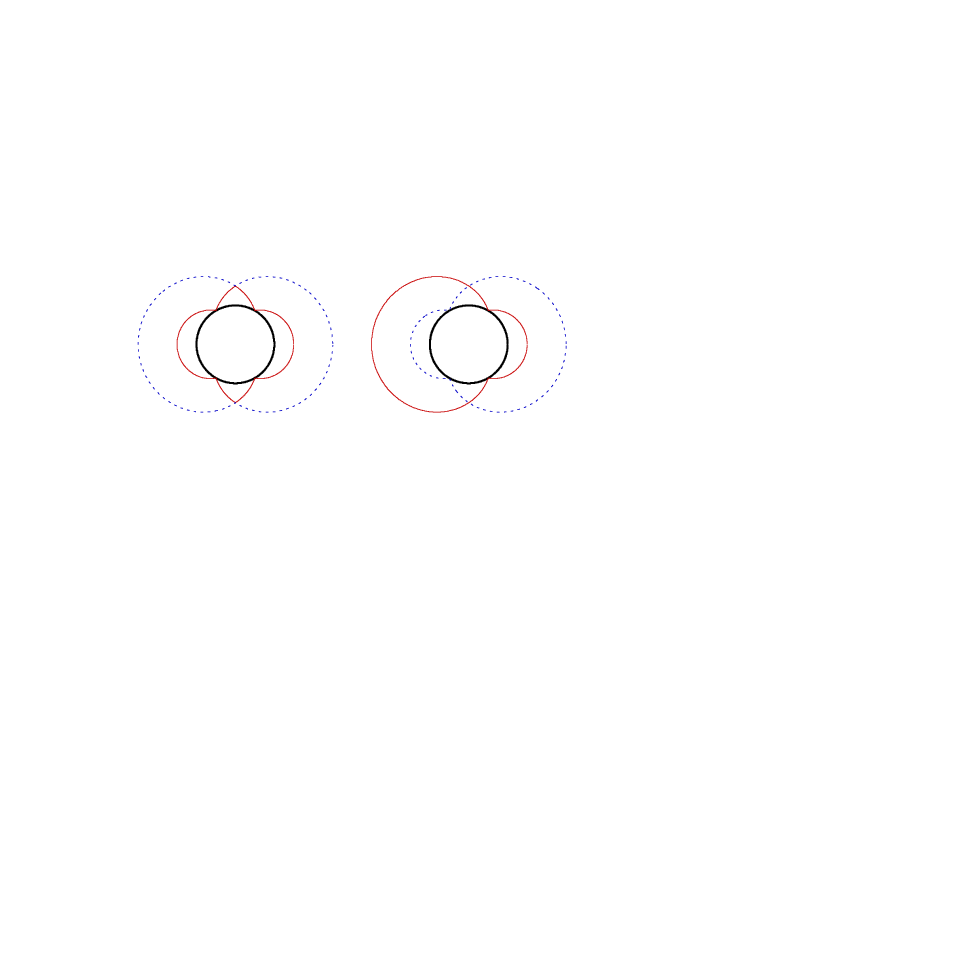
$k_{||}$ and $k_{\perp}$ (used below) are momenta parallel and perpendicular to the Fermi surface at the node. The upper branch, which is degenerate with the lower branch on the line $k_{x}=0$ between each pair of nodes, is properly included with this linearisation of the gap function. Therefore, we relabel the two branches of the gap function as shown in Fig. 1. Thus for any function we have

Each branch 1 and 2 has two cusp point nodes and the contribution to the excitation spectrum from each branch is equal. With this picture in mind, we now calculate the density of states and the transport coefficients.