Magnetized String Cosmological Model in Cylindrically Symmetric Inhomogeneous Universe with Variable Cosmological-Term $\Lambda$

Cosmic strings play an important role in the study of the early universe. These strings arise during the phase transition after the big bang explosion as the temperature goes down below some critical temperature as predicted by grand unified theories [1]${-}$ [5]. It is believed that cosmic strings give rise to density perturbations which lead to formation of galaxies [6]. These cosmic strings have stress energy and couple to the gravitational field. Therefore, it is interesting to study the gravitational effect which arises from strings. The general treatment of strings was initiated by Letelier [7, 8] and Stachel [9]. The occurrence of magnetic fields on galactic scale is well-established fact today, and their importance for a variety of astrophysical phenomena is generally acknowledged as pointed out Zel’dovich [10]. Also Harrison [11] has suggested that magnetic field could have a cosmological origin. As a natural consequences, we should include magnetic fields in the energy-momentum tensor of the early universe. The choice of anisotropic cosmological models in Einstein system of field equations leads to the cosmological models more general than Robertson-Walker model [12]. The presence of primordial magnetic fields in the early stages of the evolution of the universe has been discussed by several authors (Misner, Thorne and Wheeler [13]; Asseo and Sol [14]; Pudritz and Silk [15]; Kim, Tribble, and Kronberg [16]; Perley and Taylor [17]; Kronberg, Perry and Zukowski [18]; Wolfe, Lanzetta and Oren [19]; Kulsrud, Cen, Ostriker and Ryu [20]; Barrow [21]). Melvin [22], in his cosmological solution for dust and electromagnetic field suggested that during the evolution of the universe, the matter was in a highly ionized state and was smoothly coupled with the field, subsequently forming neutral matter as a result of universe expansion. Hence the presence of magnetic field in string dust universe is not unrealistic.

Benerjee et al. [23] have investigated an axially symmetric Bianchi type I string dust cosmological model in presence and absence of magnetic field. The string cosmological models with a magnetic field are also discussed by Chakraborty [24], Tikekar and Patel [25, 26]. Patel and Maharaj [27] investigated stationary rotating world model with magnetic field. Ram and Singh [28] obtained some new exact solution of string cosmology with and without a source free magnetic field for Bianchi type I space-time in the different basic form considered by Carminati and McIntosh [29]. Singh and Singh [30] investigated string cosmological models with magnetic field in the context of space-time with $G_{3}$ symmetry. Singh [31] has studied string cosmology with electromagnetic fields in Bianchi type-II, -VIII and -IX space-times. Lidsey, Wands and Copeland [32] have reviewed aspects of super string cosmology with the emphasis on the cosmological implications of duality symmetries in the theory. Bali et al. [33, 34, 35] have investigated Bianchi type I magnetized string cosmological models.

Cylindrically symmetric space-time play an important role in the study of the universe on a scale in which anisotropy and inhomogeneity are not ignored. Inhomogeneous cylindrically symmetric cosmological models have significant contribution in understanding some essential features of the universe such as the formation of galaxies during the early stages of their evolution. Bali and Tyagi [36] and Pradhan et al. [37, 38] have investigated cylindrically symmetric inhomogeneous cosmological models in presence of electromagnetic field. Barrow and Kunze [39, 40] found a wide class of exact cylindrically symmetric flat and open inhomogeneous string universes. In their solutions all physical quantities depend on at most one space coordinate and the time. The case of cylindrical symmetry is natural because of the mathematical simplicity of the field equations whenever there exists a direction in which the pressure equal to energy density.

In modern cosmological theories, a dynamic cosmological term $\Lambda(t)$ remains a focal point of interest as it solves the cosmological constant problem in a natural way. There are significant observational evidence for the detection of Einstein’s cosmological constant, $\Lambda$ or a component of material content of the universe that varies slowly with time and space to act like $\Lambda$. A wide range of observations now compellingly suggest that the universe possesses a non-zero cosmological term [41]. In the context of quantum field theory, a cosmological term corresponds to the energy density of vacuum. The birth of the universe has been attributed to an excited vacuum fluctuation triggering off an inflationary expansion followed by the super-cooling. The release of locked up vacuum energy results in subsequent reheating. The cosmological term, which is measure of the energy of empty space, provides a repulsive force opposing the gravitational pull between the galaxies. If the cosmological term exists, the energy it represents counts as mass because mass and energy are equivalent. If the cosmological term is large enough, its energy plus the matter in the universe could lead to inflation. Unlike standard inflation, a universe with a cosmological term would expand faster with time because of the push from the cosmological term [42]. Some of the recent discussions on the cosmological constant “problem” and on cosmology with a time-varying cosmological constant by Ratra and Peebles [43], Dolgov [44] and Sahni and Starobinsky [45] point out that in the absence of any interaction with matter or radiation, the cosmological constant remains a “constant”. However, in the presence of interactions with matter or radiation, a solution of Einstein equations and the assumed equation of covariant conservation of stress-energy with a time-varying $\Lambda$ can be found. This entails that energy has to be conserved by a decrease in the energy density of the vacuum component followed by a corresponding increase in the energy density of matter or radiation (see also Weinberg [46], Carroll, Press and Turner [47], Peebles [48], Padmanabhan [49] and Pradhan et al. [50] ).

Recent observations by Perlmutter et al. [51] and Riess et al. [52] strongly favour a significant and a positive value of $\Lambda$ with magnitude $\Lambda(G\hbar/c^{3})\approx 10^{-123}$. Their study is based on more than $50$ type Ia supernovae with red-shifts in the range $0.10\leq z\leq 0.83$ and these suggest Friedmann models with negative pressure matter such as a cosmological constant $(\Lambda)$, domain walls or cosmic strings (Vilenkin [53], Garnavich et al. [54]). Recently, Carmeli and Kuzmenko [55] have shown that the cosmological relativistic theory predicts the value for cosmological constant $\Lambda=1.934\times 10^{-35}s^{-2}$. This value of “$\Lambda$” is in excellent agreement with the recent estimates of the High-Z Supernova Team and Supernova Cosmological Project (Garnavich et al. [54]; Perlmutter et al. [51]; Riess et al. [52]; Schmidt et al. [56]). In Ref. [57] Riess et al. have recently presented an analysis of 156 SNe including a few at $z>1.3$ from the Hubble Space Telescope (HST) “GOOD ACS” Treasury survey. They conclude to the evidence for present acceleration $q_{0}<0$ $(q_{0}\approx-0.7)$. Observations (Knop et al. [58]; Riess et al., [57]) of Type Ia Supernovae (SNe) allow us to probe the expansion history of the universe leading to the conclusion that the expansion of the universe is accelerating.

Recently Baysal et al. [59] have investigated some string cosmological models in cylindrically symmetric inhomogeneous universe. Motivated by the situation discussed above, in this paper, we have generalized these solutions by including electromagnetic field tensor, pressure and cosmological term varying with time. We have taken strings and electromagnetic field together as the source gravitational field as magnetic field are anisotropic stress source and low strings are one of anisotropic stress source as well. The paper is organized as follows. The metric and the field equations are presented in Section 2. In Section 3, we deal with the solution of the field equations in presence of perfect fluid with electromagnetic field and variable cosmological term. Section 4 describes some physical and geometric properties of the universe. Finally in Section 5 concluding remarks are given.

We consider the metric in the form

$$ds^{2}=A^{2}(dx^{2}-dt^{2})+B^{2}dy^{2}+C^{2}dz^{2},$$

(1)

where $A$, $B$ and $C$ are functions of $x$ and $t$. The energy momentum tensor for the cloud of strings with perfect fluid and electromagnetic field has the form

$$T^{j}_{i}=(\rho+p)u_{i}u^{j}+pg^{j}_{i}-\lambda x_{i}x^{j}+E^{j}_{i},$$

(2)

where $u_{i}$ and $x_{i}$ satisfy conditions

$$u^{i}u_{i}=-x^{i}x_{i}=-1,$$

(3)

and

$$u^{i}x_{i}=0.$$

(4)

Here $\rho$ is the rest energy density of the cloud of strings, $p$ is the isotropic pressure, $\lambda$ is the tension density of the strings, $x^{i}$ is a unit space-like vector representing the direction of strings so that $x^{1}=0=x^{2}=x^{4}$ and $x^{3}\neq 0$, and $u^{i}$ is the four velocity vector satisfying the following conditions

$$g_{ij}u^{i}u^{j}=-1.$$

(5)

In Eq. (2), $E^{j}_{i}$ is the electromagnetic field given by Lichnerowicz [60]

$$E^{j}_{i}=\bar{\mu}\left[h_{l}h^{l}\left(u_{i}u^{j}+\frac{1}{2}g^{j}_{i}\right)-h_{i}h^{j}\right],$$

(6)

where $\bar{\mu}$ is the magnetic permeability and $h_{i}$ the magnetic flux vector defined by

$$h_{i}=\frac{1}{\bar{\mu}}\,{{}^{*}}F_{ji}u^{j},$$

(7)

where the dual electromagnetic field tensor ${}^{*}F_{ij}$ is defined by Synge [61]

$$^{*}F_{ij}=\frac{\sqrt{-g}}{2}\epsilon_{ijkl}F^{kl}.$$

(8)

Here $F_{ij}$ is the electromagnetic field tensor and $\epsilon_{ijkl}$ is the Levi-Civita tensor density.

In the present scenario, the comoving coordinates are taken as

$$u^{i}=\left(0,0,0,\frac{1}{A}\right).$$

(9)

The incident magnetic field is taken along x-axis so that

$$h_{1}\neq 0,h_{2}=0=h_{3}=h_{4}$$

(10)

The first set of Maxwell’s equations

$$F_{ij;k}+F_{jk,i}+F_{ki;j}=0,$$

(11)

lead to

$$F_{23}=\mbox{constant}=H\mbox{(say)}.$$

(12)

The semicolon represents a covariant differentiation. Here $F_{12}=F_{24}=F_{34}=0$ due to assumption of infinite electromagnetic conductivity. The only non-vanishing component of $F_{ij}$ is $F_{23}$.

The Einstein’s field equations (with $\frac{8\pi G}{c^{4}}=1$)

$$R^{j}_{i}-\frac{1}{2}Rg^{j}_{i}+\Lambda g^{j}_{i}=-T^{j}_{i},$$

(13)

for the line-element (1) lead to the following system of equations:

$$\frac{1}{A^{2}}\left[-\frac{B_{44}}{B}-\frac{C_{44}}{C}+\frac{A_{4}}{A}\left(\frac{B_{4}}{B}+\frac{C_{4}}{C}\right)+\frac{A_{1}}{A}\left(\frac{B_{1}}{B}+\frac{C_{1}}{C}\right)+\frac{B_{1}C_{1}}{BC}-\frac{B_{4}C_{4}}{BC}\right]$$

$$=p-\lambda-\frac{H^{2}}{2\bar{\mu}B^{2}C^{2}}+\Lambda,$$

(14)

$$\frac{1}{A^{2}}\left[-\left(\frac{A_{4}}{A}\right)_{4}+\left(\frac{A_{1}}{A}\right)_{1}-\frac{C_{44}}{C}+\frac{C_{11}}{C}\right]=p+\frac{H^{2}}{2\bar{\mu}B^{2}C^{2}}+\Lambda,$$

(15)

$$\frac{1}{A^{2}}\left[-\left(\frac{A_{4}}{A}\right)_{4}+\left(\frac{A_{1}}{A}\right)_{1}-\frac{B_{44}}{B}+\frac{B_{11}}{B}\right]=p+\frac{H^{2}}{2\bar{\mu}B^{2}C^{2}}+\Lambda,$$

(16)

$$\frac{1}{A^{2}}\left[-\frac{B_{11}}{B}-\frac{C_{11}}{C}+\frac{A_{1}}{A}\left(\frac{B_{1}}{B}+\frac{C_{1}}{C}\right)+\frac{A_{4}}{A}\left(\frac{B_{4}}{B}+\frac{C_{4}}{C}\right)-\frac{B_{1}C_{1}}{BC}+\frac{B_{4}C_{4}}{BC}\right]$$

$$=\rho+\frac{H^{2}}{2\bar{\mu}B^{2}C^{2}}-\Lambda,$$

(17)

$$\frac{B_{14}}{B}+\frac{C_{14}}{C}-\frac{A_{4}}{A}\left(\frac{B_{1}}{B}+\frac{C_{1}}{C}\right)-\frac{A_{1}}{A}\left(\frac{B_{4}}{B}+\frac{C_{4}}{C}\right)=0,$$

(18)

where the sub indices $1$ and $4$ in A, B, C and elsewhere denote ordinary differentiation with respect to $x$ and $t$ respectively.

The rotation $\omega^{2}$ is identically zero. The scalar expansion $\theta$, shear scalar $\sigma^{2}$, acceleration vector $\dot{u}_{i}$ and proper volume $V^{3}$ are respectively found to have the following expressions:

$$\theta=u^{i}_{;i}=\frac{1}{A}\left(\frac{A_{4}}{A}+\frac{B_{4}}{B}+\frac{C_{4}}{C}\right),$$

(19)

$$\sigma^{2}=\frac{1}{2}\sigma_{ij}\sigma^{ij}=\frac{1}{3}\theta^{2}-\frac{1}{A^{2}}\left(\frac{A_{4}B_{4}}{AB}+\frac{B_{4}C_{4}}{BC}+\frac{C_{4}A_{4}}{CA}\right),$$

(20)

$$\dot{u}_{i}=u_{i;j}u^{j}=\left(\frac{A_{1}}{A},0,0,0\right)$$

(21)

$$V^{3}=\sqrt{-g}=A^{2}BC,$$

(22)

where $g$ is the determinant of the metric (1).

As in the case of general-relativistic cosmologies, the introduction of inhomogeneities into the string cosmological equations produces a considerable increase in mathematical difficulty: non-linear partial differential equations must now be solved. In practice, this means that we must proceed either by means of approximations which render the non- linearities tractable, or we must introduce particular symmetries into the metric of the space-time in order to reduce the number of degrees of freedom which the inhomogeneities can exploit.

Here to get a determinate solution, let us assume that expansion ($\theta$) in the model is proportional to the eigen value $\sigma^{1}~~_{1}$ of the shear tensor $\sigma^{i}~~_{j}$. This condition leads to

$$A=(BC)^{n},$$

(23)

where $n$ is a constant. Equations (15) and (16) lead to

$$\frac{B_{44}}{B}-\frac{B_{11}}{B}=\frac{C_{44}}{C}-\frac{C_{11}}{C}.$$

(24)

Using (23) in (18), yields

$$\frac{B_{41}}{B}+\frac{C_{41}}{C}-2n\left(\frac{B_{4}}{B}+\frac{C_{4}}{C}\right)\left(\frac{B_{1}}{B}+\frac{C_{1}}{C}\right)=0.$$

(25)

To find out deterministic solutions, we consider

$$B=f(x)g(t)~~\mbox{and}~~C=h(x)k(t).$$

(26)

In this case equation (25) reduces to

$$\frac{f_{1}/f}{h_{1}/h}=-\frac{(2n-1)(k_{4}/k)+2n(g_{4}/g)}{(2n-1)(g_{4}/g)+2n(k_{4}/k)}=K\mbox{(constant)},$$

(27)

which leads to

$$\frac{f_{1}}{f}=K\frac{h_{1}}{h}$$

(28)

and

$$\frac{k_{4}/k}{g_{4}/g}=\frac{K-2nK-2n}{2nK+2n-1}=a\mbox{(constant)}.$$

(29)

From Eqs. (28) and (29), we obtain

$$f=\alpha h^{K}$$

(30)

and

$$k=\delta g^{a},$$

(31)

where $\alpha$ and $\delta$ are integrating constants. Eq. (24) and (26) reduce to

$$\frac{g_{44}}{g}-\frac{k_{44}}{k}=\frac{f_{11}}{f}-\frac{h_{11}}{h}=N,$$

(32)

where $N$ is a constant. Eqs. (29) and (32) lead to

$$gg_{44}+ag_{4}^{2}=-\frac{N}{a-1}g^{2},$$

(33)

which leads to

$$g=\beta^{\frac{1}{a+1}}\sinh^{\frac{1}{a+1}}(bt+t_{0}),$$

(34)

where $\beta$ and $t_{0}$ are constants of integration and

$$b=\sqrt{\frac{N(a+1)}{1-a}}.$$

Thus from Eq. (31) we get

$$k=\delta\beta^{\frac{a}{a+1}}\sinh^{\frac{a}{a+1}}(bt+t_{0}).$$

(35)

From Eqs. (27) and (32), we obtain

$$hh_{11}+Kh_{1}^{2}=\frac{N}{K-1}h^{2},$$

(36)

which leads to

$$h=\ell^{\frac{1}{K+1}}\sinh^{\frac{1}{K+1}}(rx+x_{0}),$$

(37)

where $\ell$ and $x_{0}$ are constants of integration and

$$r=\sqrt{\frac{N(K+1)}{K-1}}.$$

Hence from Eq. (30) we have

$$f=\alpha\ell^{\frac{K}{K+1}}\sinh^{\frac{K}{K+1}}(rx+x_{0}).$$

(38)

It is worth mentioned here that equations (33) and (36) are fundamental basic differential equations for which we have reported new solutions given by equations (34) and (37).

Thus, we obtain

$$B=fg=Q\sinh^{\frac{K}{K+1}}(rx+x_{0})\sinh^{\frac{1}{a+1}}(bt+t_{0}),$$

(39)

$$C=hk=R\sinh^{\frac{1}{K+1}}(rx+x_{0})\sinh^{\frac{a}{a+1}}(bt+t_{0}),$$

(40)

and

$$A=(BC)^{n}=M\sinh^{n}(rx+x_{0})\sinh^{n}(bt+t_{0}),$$

(41)

where

$$Q=\alpha\beta^{\frac{1}{a+1}}\ell^{\frac{K}{K+1}},$$

$$R=\delta\beta^{\frac{a}{a+1}}\ell^{\frac{1}{K+1}},$$

$$M=(QR)^{n}.$$

Hence the geometry of the space-time (1) takes the form

$$ds^{2}=M^{2}\sinh^{2n}(rx+x_{0})\sinh^{2n}(bt+t_{0})(dx^{2}-dt^{2})+$$

$$Q^{2}\sinh^{\frac{2K}{K+1}}(rx+x_{0})\sinh^{\frac{2}{a+1}}(bt+t_{0})dy^{2}+$$

$$R^{2}\sinh^{\frac{2}{K+1}}(rx+x_{0})\sinh^{\frac{2a}{a+1}}(bt+t_{0})dz^{2}.$$

(42)

By using the following transformation

$$rX=rx+x_{0},$$

$$Y=Qy,$$

$$Z=Rz$$

$$bT=bt+t_{0}$$

(43)

the metric (42) reduces to

$$ds^{2}=M^{2}\sinh^{2n}(rX)\sinh^{2n}(bT)(dX^{2}-dT^{2})+$$

$$\sinh^{\frac{2K}{K+1}}(rX)\sinh^{\frac{2}{a+1}}(bT)dY^{2}+\sinh^{\frac{2}{K+1}}(rX)\sinh^{\frac{2a}{a+1}}(bT)dZ^{2}.$$

(44)

In this case the physical parameters, i.e. the pressure $(p)$, the energy density $(\rho)$, the string tension density $(\lambda)$, the particle density $(\rho_{p})$ and the cosmological term $\Lambda(t)$ for the model (42) are given by

$$p=\frac{1}{M^{2}\sinh^{2n}(bT)\sinh^{2n}(rX)}\Biggl[b^{2}\left\{n+\frac{a}{(a+1)^{2}}\right\}\coth^{2}(bT)$$

$$-\,r^{2}\left\{n+\frac{K}{(K+1)^{2}}\right\}\coth^{2}(rX)-b^{2}\left\{n+\frac{1}{(a+1)}\right\}+r^{2}\left\{n+\frac{K}{(K+1)}\right\}\Biggr]$$

$$-\,\frac{\kappa}{\sinh^{2}(bT)\sinh^{2}(rX)}-\Lambda,$$

(45)

$$\lambda=\frac{1}{M^{2}\sinh^{2n}(bT)\sinh^{2n}(rX)}\Biggl[r^{2}\left\{n+\frac{K}{(K+1)}\right\}-\,b^{2}\left\{n+1+\frac{1}{(a+1)}\right\}$$

$$-\,2r^{2}\left\{n+\frac{K}{(K+1)^{2}}\right\}\coth^{2}(rX)\Biggr]-\,\frac{2\kappa}{\sinh^{2}(bT)\sinh^{2}(rX)},$$

(46)

$$\rho=\frac{1}{M^{2}\sinh^{2n}(bT)\sinh^{2n}(rX)}\Biggl[b^{2}\left\{n+\frac{a}{(a+1)^{2}}\right\}\coth^{2}(bT)$$

$$+\,r^{2}\left\{n+\frac{K}{(K+1)^{2}}\right\}\coth^{2}(rX)-r^{2}\Biggr]-\,\frac{\kappa}{\sinh^{2}(bT)\sinh^{2}(rX)}+\Lambda,$$

(47)

$$\rho_{p}=\rho-\lambda=\frac{1}{M^{2}\sinh^{2n}(bT)\sinh^{2n}(rX)}\Biggl[b^{2}\left\{n+\frac{a}{(a+1)^{2}}\right\}\coth^{2}(bT)$$

$$+\,3r^{2}\left\{n+\frac{K}{(K+1)^{2}}\right\}\coth^{2}(rX)+b^{2}\left\{n-1+\frac{1}{(a+1)}\right\}$$

$$-\,r^{2}\left\{n+1+\frac{K}{(K+1)}\right\}\Biggr]+\,\frac{\kappa}{\sinh^{2}(bT)\sinh^{2}(rX)}+\Lambda,$$

(48)

where

$$\kappa=\frac{H^{2}}{2\bar{\mu}}.$$

For the specification of $\Lambda$, we assume that the fluid obeys an equation of state of the form

$$p=\gamma\rho,$$

(49)

where $\gamma(0\leq\gamma\leq 1)$ is a constant.
From Eqs. (45), (47) and (49), we obtain

$$\Lambda=\frac{1}{(1-\gamma)M^{2}\sinh^{2n}(bT)\sinh^{2n}(rX)}\Biggl[(1-\gamma)b^{2}\left\{n+\frac{a}{(a+1)^{2}}\right\}\coth^{2}(bT)$$

$$-\,(1+\gamma)r^{2}\left\{n+\frac{K}{(K+1)^{2}}\right\}\coth^{2}(rX)-b^{2}\left\{n+\frac{1}{(a+1)}\right\}$$

$$+\,r^{2}\left\{n+\frac{K}{(K+1)}\right\}-\gamma r\Biggr]-\,\frac{\kappa}{\sinh^{2}(bT)\sinh^{2}(rX)}.$$

(50)

From Eq. (47), we note that $\rho(t)$ is a decreasing function of time and $\rho>0$ for all times. Figure 1 shows this behaviour of energy density.

In spite of homogeneity at large scale our universe is inhomogeneous at small scales, so physical quantities being position dependent are more natural in our observable universe if we do not go to super high scale. This result shows this kind of physical importance. In recent time the $\Lambda$-term has interested theoreticians and observers for various reasons. The nontrivial role of the vacuum in the early universe generate a $\Lambda$-term that leads to inflationary phase. Observationally, this term provides an additional parameter to accommodate conflicting data on the values of the Hubble constant, the deceleration parameter, the density parameter and the age of the universe (for example, see the references [62, 63]). Assuming that $\Lambda$ owes its origin to vacuum interactions, as suggested in particular by Sakharov [64], it follows that it would in general be a function of space and time coordinates, rather than a strict constant. In a homogeneous universe $\Lambda$ will be at most time dependent [65]. In our case this approach can generate $\Lambda$ that varies both with space and time. In considering the nature of local massive objects, however, the space dependence of $\Lambda$ cannot be ignored. For details discussion, the readers are advised to see the references (Narlikar, Pecker and Vigier [66], Ray and Ray [67], Tiwari, Ray and Bhadra [68]).

The behaviour of the universe in this model will be determined by the cosmological term $\Lambda$ ; this term has the same effect as a uniform mass density $\rho_{eff}=-\Lambda/4\pi G$, which is constant in space and time. A positive value of $\Lambda$ corresponds to a negative effective mass density (repulsion). Hence, we expect that in the universe with a positive value of $\Lambda$, the expansion will tend to accelerate; whereas in the universe with negative value of $\Lambda$, the expansion will slow down, stop and reverse. From Eq. 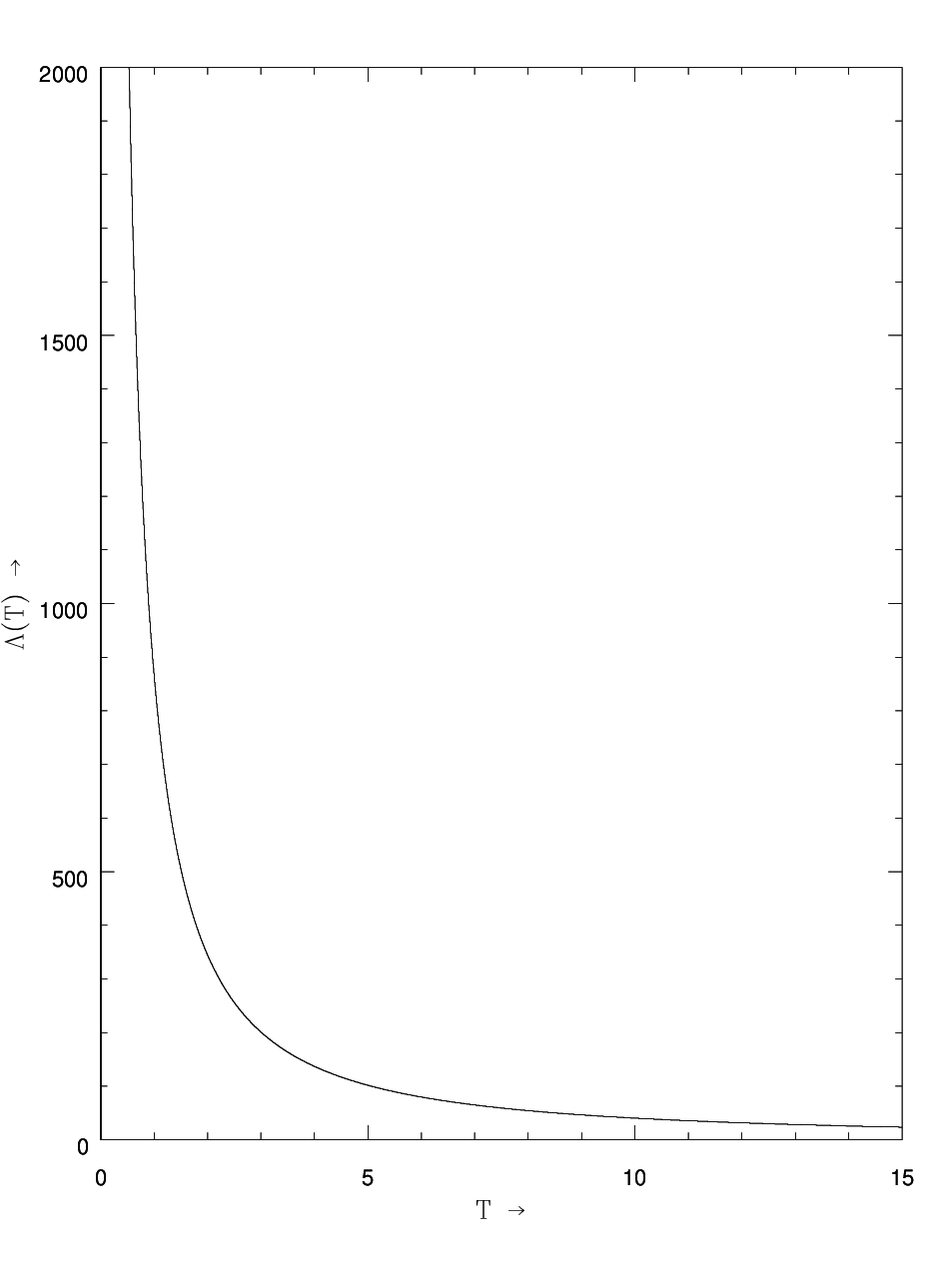(50), we see that the cosmological term $\Lambda$ is a decreasing function of time and it approaches a small positive value as time increases more and more. From Figure 2 we note this behaviour of cosmological term $\Lambda$. Recent cosmological observations (Garnavich et al. [54], Perlmutter et al. [51], Riess et al. [52, 57], Schmidt et al. [56]) suggest the existence of a positive cosmological constant $\Lambda$ with the magnitude $\Lambda(G\hbar/c^{3})\approx 10^{-123}$. These observations on magnitude and red-shift of type Ia supernova suggest that our universe may be an accelerating one with induced cosmological density through the cosmological $\Lambda$-term. Thus, our model is consistent with the results of recent observations.

The kinematical quantities , i.e. the scalar of expansion $(\theta)$, shear tensor $(\sigma)$, the acceleration vector $(\dot{u}_{i})$ and the proper volume $(V^{3})$ for the model (42) are given by

$$\theta=\frac{b(n+1)\coth(bT)}{M\sinh^{n}(bT)\sinh^{n}(rX)},$$

(51)

$$\sigma^{2}=\frac{b^{2}\coth^{2}(bT)[(a+1)^{2}(n^{2}-n+1)-3a]}{3(a+1)^{2}M^{2}\sinh^{2n}(bT)\sinh^{2n}(rX)},$$

(52)

$$\dot{u}_{i}=(nr\coth(rX),0,0,0),$$

(53)

$$V^{3}=\sinh^{2n+1}(bT)\sinh^{2n+1}(rX).$$

(54)

From Eqs. (47) and (48), we obtain

$$\frac{\sigma^{2}}{\theta^{2}}=\frac{(a+1)^{2}(n^{2}-n+1)-3a}{3(n+1)^{2}(a+1)^{2}}=\mbox{constant}.$$

(55)

The dominant energy conditions (Hawking and Ellis [69])

$$(i)~~\rho-p\geq 0~~~(ii)~~\rho+p\geq 0$$

lead to

$$2r^{2}\left\{n+\frac{K}{(K+1)^{2}}\right\}\coth^{2}(rX)-r^{2}\left\{n+1+\frac{K}{K+1}\right\}$$

$$+\,b^{2}\left\{n+\frac{1}{a+1}\right\}+2\Lambda M^{2}\sinh^{2n}(bT)\sinh^{2n}(rX)\geq 0,$$

(56)

and

$$2b^{2}\left\{n+\frac{a}{(a+1)^{2}}\right\}\coth^{2}(bT)+r^{2}\left\{n-1+\frac{K}{K+1}\right\}$$

$$-\,b^{2}\left\{n+\frac{1}{a+1}\right\}\geq 2M^{2}\kappa\sinh^{2n-2}(bT)\sinh^{2n-2}(rX).$$

(57)

The reality conditions (Ellis [70])

$$(i)~~\rho+p>0,~~~(ii)~~\rho+3p>0,$$

lead to

$$2b^{2}\left\{n+\frac{a}{(a+1)^{2}}\right\}\coth^{2}(bT)+r^{2}\left\{n-1+\frac{K}{K+1}\right\}$$

$$-\,b^{2}\left\{n+\frac{1}{a+1}\right\}>2M^{2}\kappa\sinh^{2n-2}(bT)\sinh^{2n-2}(rX),$$

(58)

and

$$4b^{2}\left\{n+\frac{a}{(a+1)^{2}}\right\}\coth^{2}(bT)-2r^{2}\left\{n+\frac{K}{(K+1)^{2}}\right\}\coth^{2}(rX)$$

$$+3r^{2}\left\{n+\frac{K}{K+1}\right\}-\,3b^{2}\left\{n+\frac{1}{a+1}\right\}-r^{2}$$

$$>4M^{2}\kappa\sinh^{2n-2}(bT)\sinh^{2n-2}(rX)+2M^{2}\Lambda\sinh^{2n}(bT)\sinh^{2n}(rX).$$

(59)

The model starts expanding with a big bang at $T=0$ and it stops expanding at $T=\infty$. In general, the model represents an expanding, shearing and non-rotating universe. Since $\frac{\sigma}{\theta}=$ constant, hence the model does not approach isotropy. When the uniform magnetic field is not present and $p=0$, $\Lambda=0$, our solution represents the solution obtained by Baysal et al. [59]. The model is accelerating. The proper volume in the model increases as $T$ increases.

In absence of the magnetic field i.e. $H=0$, the physical parameters, i.e. the pressure $(p)$, the energy density $(\rho)$, the string tension density $(\lambda)$, the particle density $(\rho_{p})$ and the cosmological term $\Lambda(t)$ for the model (44) are given by

$$p=\frac{1}{M^{2}\sinh^{2n}(bT)\sinh^{2n}(rX)}\Biggl[b^{2}\left\{n+\frac{a}{(a+1)^{2}}\right\}\coth^{2}(bT)$$

$$-\,r^{2}\left\{n+\frac{K}{(K+1)^{2}}\right\}\coth^{2}(rX)-b^{2}\left\{n+\frac{1}{(a+1)}\right\}+r^{2}\left\{n+\frac{K}{(K+1)}\right\}\Biggr]-\Lambda,$$

(60)

$$\lambda=\frac{1}{M^{2}\sinh^{2n}(bT)\sinh^{2n}(rX)}\Biggl[r^{2}\left\{n+\frac{K}{(K+1)}\right\}-\,b^{2}\left\{n+1+\frac{1}{(a+1)}\right\}$$

$$-\,2r^{2}\left\{n+\frac{K}{(K+1)^{2}}\right\}\coth^{2}(rX)\Biggr],$$

(61)

$$\rho=\frac{1}{M^{2}\sinh^{2n}(bT)\sinh^{2n}(rX)}\Biggl[b^{2}\left\{n+\frac{a}{(a+1)^{2}}\right\}\coth^{2}(bT)$$

$$+\,r^{2}\left\{n+\frac{K}{(K+1)^{2}}\right\}\coth^{2}(rX)-r^{2}\Biggr]+\Lambda,$$

(62)

$$\rho_{p}=\rho-\lambda=\frac{1}{M^{2}\sinh^{2n}(bT)\sinh^{2n}(rX)}\Biggl[b^{2}\left\{n+\frac{a}{(a+1)^{2}}\right\}\coth^{2}(bT)$$

$$+\,3r^{2}\left\{n+\frac{K}{(K+1)^{2}}\right\}\coth^{2}(rX)+b^{2}\left\{n-1+\frac{1}{(a+1)}\right\}$$

$$-\,r^{2}\left\{n+1+\frac{K}{(K+1)}\right\}\Biggr]+\Lambda.$$

(63)

By using the equation of state (49) in Eqs. (60) and (62), we obtain

$$\Lambda=\frac{1}{(1-\gamma)M^{2}\sinh^{2n}(bT)\sinh^{2n}(rX)}\Biggl[(1-\gamma)b^{2}\left\{n+\frac{a}{(a+1)^{2}}\right\}\coth^{2}(bT)$$

$$-\,(1+\gamma)r^{2}\left\{n+\frac{K}{(K+1)^{2}}\right\}\coth^{2}(rX)-b^{2}\left\{n+\frac{1}{(a+1)}\right\}$$

$$+\,r^{2}\left\{n+\frac{K}{(K+1)}\right\}-\gamma r\Biggr].$$

(64)

We observe that in absence of the magnetic field, the expressions for Kinematical quantities for the model (42) are unchanged.

From Eq. (62), we note that $\rho(t)$ is a decreasing function of time and $\rho>0$ for all times. Figure 3 shows this behaviour of energy density. From Eq. (64), we see that the cosmological term $\Lambda$ is a decreasing function of time and it approaches a small positive value as time increases more and more which matches with recent observations. From Figure 4 we note this behaviour of cosmological term $\Lambda$. When we set $p=0$ and $\Lambda=0$, our solution represents the solution obtained by Baysal et al. [59]).

We have obtained a new cylindrically symmetric inhomogeneous cosmological model of uniform electromagnetic perfect fluid as the source of matter where the cosmological constant is varying with time. Generally the model represents an expanding, shearing and non-rotating universe in which the flow vector is geodetic. The model does not approach isotropy.

In presence and absence of magnetic field, the cosmological terms in the models are decreasing function of time and approach a small value at late time. The values of cosmological “constant” for the models are found to be small and positive, which is supported by the results from supernovae observations recently obtained by the High-Z Supernovae Ia Team and Supernova Cosmological Project (Garnavich et al. [54], Perlmutter et al. [51], Riess et al. [52, 57], Schmidt et al. [56]). Our solutions generalize the solutions obtained by Baysal et al. [59]).

Author would like to thank the Inter-University Centre for Astronomy and Astrophysics, Pune, India for providing facility under associateship programme where this work was carried out.

References

- [1] Ya. B. Zel’dovich, I. Yu. Kobzarev and L. B. Okun, Zh. Eksp. Teor. Fiz. 67, 3 (1975); Sov. Phys.-JETP 40, 1 (1975).
- [2] T. W. B. Kibble, J. Phys. A: Math. Gen. 9, 1387 (1976).
- [3] T. W. B. Kibble, Phys. Rep. 67, 183 (1980).
- [4] A. E. Everett, Phys. Rev. 24, 858 (1981).
- [5] A. Vilenkin, Phys. Rev. D 24, 2082 (1981).
- [6] Ya. B. Zel’dovich, Mon. Not. R. Astron. Soc. 192, 663 (1980).
- [7] P. S. Letelier, Phys. Rev. D 20, 1249 (1979).
- [8] P. S. Letelier, Phys. Rev. D 28, 2414 (1983).
- [9] J. Stachel, Phys. Rev. D 21, 2171 (1980).
- [10] Ya. B. Zel’dovich, A. A. Ruzmainkin, and D. D. Sokoloff, Magnetic field in Astrophysics, Gordon and Breach, New Yark, (1983).
- [11] E. R. Harrison, Phys. Rev. Lett. 30, 188 (1973).
- [12] H. P. Robertson and A. G. Walker, Proc. London Math. Soc. 42, 90 (1936).
- [13] C. W. Misner, K. S. Thorne and J. A. Wheeler, Gravitation, W. H. Freeman, New York, (1973).
- [14] E. Asseo and H. Sol, Phys. Rep. 6, 148 (1987).
- [15] R. Pudritz and J. Silk, Astrophys. J. 342, 650 (1989).
- [16] K. T. Kim, P. G. Tribble and P. P. Kronberg, Astrophys. J. 379, 80 (1991).
- [17] R. Perley and G. Taylor, Astrophys. J. 101, 1623 (1991).
- [18] P. P. Kronberg, J. J. Perry and E. L. Zukowski, Astrophys. J. 387, 528 (1991).
- [19] A. M. Wolfe, K. Lanzetta, and A. L. Oren Astrophys. J. 388, 17 (1992).
- [20] R. Kulsrud, R. Cen, J. P. Ostriker, and D. Ryu Astrophys. J. 380, 481 (1997).
- [21] J. D. Barrow, Phys. Rev. D 55, 7451 (1997).
- [22] M. A. Melvin, Ann. New York Acad. Sci. 262, 253 (1975).
- [23] A. Banerjee, A. K. Sanyal and S. Chakraborty, Pramana-J. Phys. 34, 1 (1990).
- [24] S. Chakraborty, Ind. J. Pure Appl. Phys. 29, 31 (1980).
- [25] R. Tikekar and L. K. Patel, Gen. Rel. Grav. 24, 397 (1992).
- [26] R. Tikekar and L. K. Patel, Pramana-J. Phys. 42, 483 (1994).
- [27] L. K. Patel and S. D. Maharaj, Pramana-J. Phys. 47, 1 (1996).
- [28] S. Ram and T. K. Singh, Gen. Rel. Grav. 27, 1207 (1995).
- [29] J. Carminati and C. B. G. McIntosh, J. Phys. A: Math. Gen. 13, 953 (1980).
- [30] G. P. Singh and T. Singh, Gen. Rel. Grav. 31, 371 (1999).
- [31] G. P. Singh, Nuovo Cim. B 110, 1463 (1995); Pramana-J. Phys. 45, 189 (1995).
- [32] J. E. Lidsey, D. Wands and E. J. Copeland, Phys. Rep. 337, 343 (2000).
- [33] R. Bali and R. D. Upadhaya, Astrophys. Space Sci. 283, 97 (2003).
- [34] R. Bali and Anjali, Astrophys. Space Sci. 302, 201 (2006).
- [35] R. Bali, U. K. Pareek and A. Pradhan, Chin. Phys. Lett. 24, 2455 (2007).
- [36] R. Bali and A. Tyagi, Gen. Rel. Grav. 21, 797 (1989).
- [37] A. Pradhan, I. Chakrabarty and N. N. Saste, Int. J. Mod. Phys. D 10, 741 (2001).
- [38] A. Pradhan, P. K. Singh and K. Jotania, Czech. J. Phys. 56, 641 (2006).
- [39] J. D. Barrow and K. E. Kunze, Phys. Rev. D 56, 741 (1997).
- [40] J. D. Barrow and K. E. Kunze, Phys. Rev. D 57, 2255 (1998).
- [41] L. M. Krauss and M. S. Turner, Gen. Rel. Grav. 27, 1137 (1995).
- [42] Ken Croswell, New Scientist April, 18 (1994).
- [43] B. Ratra and P. J. E. Peebles, Phys. Rev. D 37, 3406 (1988).
- [44]
A. D. Dolgov, in The Very Early Universe, eds. G. W.
Gibbons, S. W. Hawking and S. T. C. Siklos, Cambridge University
Press, Cambridge, (1983);
A. D. Dolgov, M. V. Sazhin and Ya. B. Zeldovich, Basics of Modern Cosmology, Editions Frontiers, (1990);
A. D. Dolgov, Phys. Rev. D 55, 5881 (1997). - [45] V. Sahni and A. Starobinsky, Int. J. Mod. Phys. D 9, 373 (2000).
- [46] S. Weinberg, Gravitation and Cosmology, Wiley, New Yark, (1971).
- [47] S. M. Carroll, W. H. Press and E. L. Turner, Ann. Rev. Astron. Astrophys. 30, 499 (1992).
- [48] P. J. E. Peebles, Rev. Mod. Phys. 75, 559 (2003).
- [49]
T. Padmanabhan, Phys. Rep. 380, 235 (2003).
T. Padmanabhan,Dark Energy and Gravity, gr-qc/0705.2533 (2007). - [50]
A. Pradhan and H. R. Pandey, Int. J. Mod. Phys. D 12, 941 (2003).
A. Pradhan and O. P. Pandey, Int. J. Mod. Phys. D 12, 1299 (2003).
A. Pradhan, S. K. Srivastav and K. R. Jotania, Czech. J. Phys. 54, 255 (2004).
A. Pradhan and S. Singh, Int. J. Mod. Phys. D 13, 503 (2004).
A. Pradhan, A. K. Yadav and L. Yadav, Czech. J. Phys. 55, 503 (2005).
A. Pradhan and P. Pandey, Czech. J. Phys. 55, 749 (2005).
A. Pradhan and P. Pandey, Astrophys. J. 301, 221 (2006).
A. Pradhan, G. P. Singh and S. Kotambkar, Fizika B, 15, 57 (2006).
A. Pradhan, A. K. Singh and S. Otarod, Roman. J. Phys. 52, 445 (2007).
C. P. Singh, S. Kumar and A. Pradhan, Class. Quantum Grav. 24, 455 (2007). - [51] S. Perlmutter et al., Astrophys. J. 483, 565 (1997); Nature 391, 51 (1998); Astrophys. J. 517, 565 (1999).
- [52] A. G. Riess et al., Astron. J. 116, 1009 (1998).
- [53] A. Vilenkin, Phys. Rep. 121, 265 (1985).
- [54] P. M. Garnavich et al., Astrophys. J. 493, L53 (1998a); Astrophys. J. 509, 74 (1998b).
- [55]
M. Carmeli and T. Kuzmenko, Int. J. Theor. Phys. 41, 131 (2002);
S. Behar and M. Carmeli, Int. J. Theor. Phys. 39, 1375 (2002). - [56] B. P. Schmidt et al., Astrophys. J. 507, 46 (1998).
- [57] A. G. Riess et al., Astrophys. J. 607, 665 (2004).
- [58] R. K. Knop et al., Astrophys. J. 598, 102 (2003).
- [59] H. Baysal, I. Yavuz, I. Tarhan, U. Camci and I. Yilmaz, Turk. J. Phys. 25, 283 (2001).
- [60] A. Lichnerowica, Relativistic Hydrodynamics and Magnetohydrodynamics, W. A. Benjamin Inc., New York, p. 93 (1967).
- [61] J. L. Synge, Relativity: The General Theory, North-Holland Publ. Co., Amsterdam, p. 356 (1960).
- [62] J. Gunn and B. M. Tinsley, Nature, 257, 454 (1975).
- [63] E. J. Wampler and W. L. Burke, in New Ideas in Astronomy (Eds. F. Bertola, J. W. sulentic, and B. F. Madore), Cambridge University Press, p. 317 (1988).
- [64] A. D. Sakharov, Doklady Akad. Nauk. SSSR 177, 70 (1968) (translation, Soviet Phys. Doklady, 12, 1040 (1968)).
- [65] P. J. E. Peebles and B. Ratra, Astrophys. J. 325, L17 (1988).
- [66] J. V. Narlikar, J. -C. Pecker and J. -P. Vigier, J. Astrophys. Astr. 12, 7 (1991).
- [67] S. Ray and D. Ray, Astrophys. Space Sci. 203, 211 (1993).
- [68] R. N. Tiwari, S. Ray and S. Bhadra, Indian Pure Appl. Math. 31, 1017 (2000).
- [69] S. W. Hawking and G, F, R. Ellis, The Large-scale Structure of Space Time, Cambridge University Press, Cambridge, p. 94, (1973).
- [70] G. F. R. Ellis, General Relativity and Cosmology, ed. R. K. Sachs, Clarendon Press, p. 117 (1973).