Using rotation rates to probe age spreads in the Orion Nebula ClusterUsing rotation rates to probe age spreads in the Orion Nebula Cluster–References2007
Abstract
The radii of young pre-main-sequence (PMS) stars in the Orion Nebula Cluster (ONC) have been estimated using their rotation periods and projected equatorial velocities. Stars at a given effective temperature have a spread in their geometrically estimated projected radii that is larger than can be accounted for with a coeval model, observational uncertainties and randomly oriented rotation axes. It is shown that the required dispersion in radius (a factor of 2–3 full width half maximum) can be modelled in terms of a spread in stellar ages larger than the median age of the cluster, although the detailed star formation history cannot be uniquely determined using present data. This technique is relatively free from systematic uncertainties (binarity, extinction, variability, distance) that have hampered previous studies of the ONC star formation history using the conventional Hertzsprung-Russell diagram. However, the current ONC rotational data are biased against low luminosity objects, so the deduced dispersions in radius and inferred age are probably underestimates. In particular, the ages of a tail of PMS stars that appear to be Myr old in the Hertzsprung-Russell diagram cannot be verified with present data. If projected equatorial velocities were measured for these objects it could easily be checked whether their radii are correspondingly smaller than the bulk of the ONC population.
Keywords:
stars: formation – methods: statistical – open clusters and associations: M421 Introduction
Whether star formation takes place rapidly on dynamical timescales or is a quasi-static process in which protostellar cores take many free-fall timescales to contract is one of the important debates in theoretical star formation (e.g. Shu, Adams & Lizano 1987; Hartmann, Ballesteros-Paredes & Bergin 2001; Tassis & Mouschovias 2004; Vázquez-Semadeni et al. 2005; Tan, Krumholz & McKee 2006).
A key observational constraint on star formation timescales is the possibility of significant age spreads in young clusters and associations. Palla & Stahler (1999, 2000) have used ages estimated from the Hertzsprung-Russell (H-R) diagrams of several clusters to argue that star formation takes place over more than 10 Myr and at an accelerating rate towards the present day. Huff & Stahler (2006) show that this formation history appears to be similar in the inner and outer parts of the Orion Nebula cluster (ONC), suggesting that the acceleration was triggered by a global contraction of the parent cloud. However, these conclusions are not universally accepted. Hartmann (2001) has shown that errors in determining the luminosities of young stars, due to binarism, uncertain extinction, variability and accretion can lead to significant overestimates of the age spread in an H-R diagram and obscure the detailed star formation history.
In this paper I explore an alternative technique for estimating the extent of luminosity and (inferred) age spreads in star forming regions using pre-main-sequence (PMS) stars in the ONC as an example. Rotational periods and projected equatorial velocities can be combined to give a geometric estimate of the stellar radius multiplied by the sine of an unknown rotation axis inclination, . Assuming random axial orientations and using PMS evolutionary models, the distributions of can be modelled in terms of a dispersion in true radius and inferred age. This idea was stimulated by the work of Rhode, Herbst & Mathieu (2001), who calculated mean as a function of position in the H-R diagram, finding 3-sigma evidence that stars with lower luminosities did indeed have smaller radii. Here I provide a more sophisticated analysis of a larger dataset. This work follows closely on from the related analysis presented in Jeffries (2007), where a similar approach was used to provide a revised distance estimate for the ONC.
The data base of rotational measurements used in this paper is described in section 2. Section 3 presents the analysis methods used in this work. The results are presented in section 4 and discussed in section 5.
2 The observational database



The ONC is among the best studied star forming regions and the premier cluster for investigating star formation and early stellar evolution. It is relatively nearby, very young ( pc, 1–2 Myr – Jeffries 2007; pc – Sandstrom et al. 2007) and contains a large population of stars and brown dwarfs covering the entire (sub)stellar mass spectrum ( – see Hillenbrand 1997; Slesnick, Hillenbrand & Carpenter 2004).
Jeffries (2007) assembled a database of 95 K- and M-type PMS stars in the ONC, with model-dependent masses of about 0.2–2 and which have proper-motion or radial velocity membership credentials, spectral types and luminosities (Hillenbrand 1997), effective temperatures based on the work by Cohen & Kuhi (1979), indicators of whether objects were actively accreting (based on excess, from Hillenbrand [1997]), rotation periods (Herbst et al. 2002) and (measured by Rhode et al. [2001] or Sicilia-Aguilar et al. [2005]). The typical precision of the measurements are spectral subclass, K in effective temperature, uncertainty in the periods and % uncertainties in . The smallest values that are taken to be reliably measured are 13.6 km s-1 and 10.0 km s-1 for the Rhode et al. and Sicilia-Aguilar et al. measurements respectively.
There are various filters applied to this data and a number of possible selection effects. The most important of these with regard to possible radius or age spreads are: (i) a bias against the inclusion of classical T-Tauri stars (CTTS), because their rotation periods can be difficult to distinguish from other non-periodic variability; (ii) a bias against slowly rotating stars, either because their periods are too long to reliably detect, they are not so magnetically active or their is too small to be reliably measured; and (iii) the sample of stars which are bright enough to obtain spectroscopy is biased towards optically brighter and hence intrinsically more luminous (and probably younger) stars.
If CTTS are predominantly younger than non-accreting weak-lined T-Tauri stars (WTTS) then the first effect will bias the sample towards older ages. The second effect is more complicated. As PMS stars contract they spin-up, but they may also lose angular momentum through winds or star-disc interactions as they get older. The longer period stars that remain in our sample appear to have larger radii on average (from radii estimated by Hillenbrand 1997) and may be younger. On the other hand, at a given rotation period a smaller (older) star will have a lower . Therefore these selection effects probably bias our sample against the inclusion of some of the youngest and oldest stars. Finally, any bias against low-luminosity stars will potentially exclude older stars, especially in the lowest mass objects in our sample. The discussion of completeness in Hillenbrand (1997) suggests that any incompleteness in the stars with spectroscopy will arise from the requirements of obtaining using high resolution spectroscopy, which is restricted to brighter stars. Spectral types can be obtained using low resolution spectroscopy for much fainter objects.
An illustration of these potential effects is provided by comparing the H-R diagrams for our “rotation sample” and for proper-motion selected ONC members with temperatures and luminosities from Hillenbrand (1997). The H-R diagram is shown in Fig. 1, along with isochrones from D’Antona & Mazzitelli (1997). The luminosities from Hillenbrand (1997) have been adjusted to correspond to the 392 pc found by Jeffries (2007), rather than the 470 pc assumed by Hillenbrand (1997).
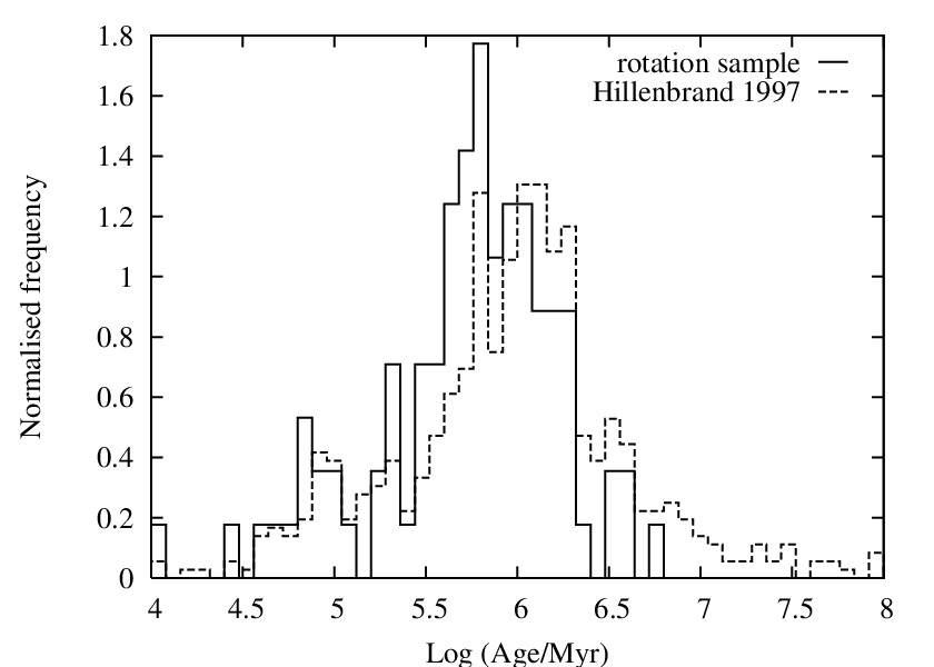
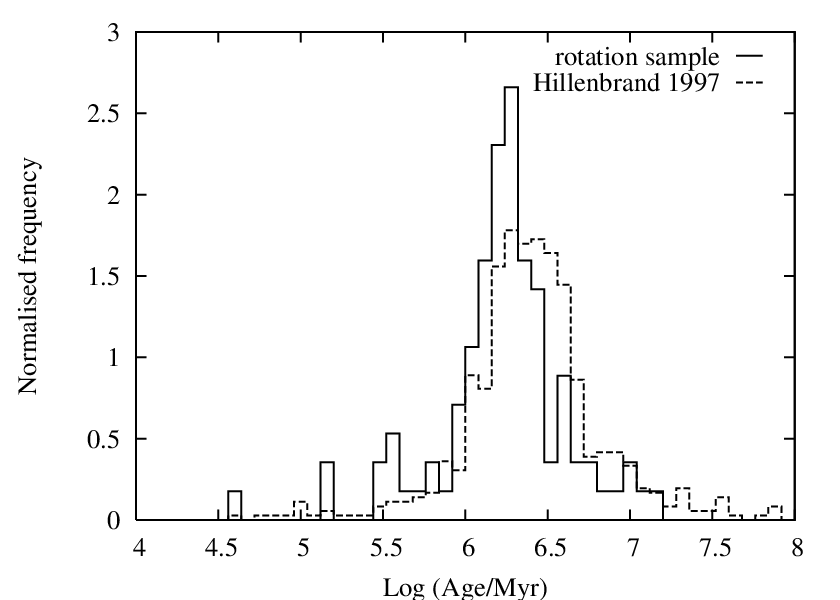
Model-dependent PMS stellar ages are estimated from these isochrones. Histograms of age are shown in Fig. 2 for the rotation sample and the full ONC sample, using linear and logarithmic age bins. The median ages are 0.62 Myr and 1.03 Myr for the rotation sample and the full sample respectively. The linearly binned age distribution of the Hillenbrand (1997) sample in Fig. 2 shows the pseudo-exponential decline characterised as “accelerating star formation” by Palla & Stahler (1999). This translates into a peak in the number of stars per logarithmic age interval at around 1 Myr. Fig. 2 also demonstrates that the tail of “older” ( Myr) stars appears to be absent from the rotation sample. A Kolmogorov-Smirnov (K-S) test suggests that there is a per cent probability that the two age distributions are consistent. This selection effect arises chiefly from the bias towards brighter targets. Some of the age bias might be thought to arise because older, smaller objects could have unresolveable (see Rebull, Wolff & Strom 2004). However, the H-R diagram-based age distribution for objects which have unresolved but otherwise match the sample selection criteria is in fact similar to that of the rotation sample.
Stars in the rotation sample are classified as CTTS or WTTS on the basis of whether their colour excess is greater or less than 0.3 mag (see Hillenbrand et al. 1998). A K-S test on the age distributions of these two populations reveals no significant evidence for a difference.
The age distributions in Fig. 2 are of course model dependent. I have repeated these exercises using the Siess, Dufour & Forestini (2000) models (the variety) and these are shown in Fig. 3. The Siess et al. models give older ages and the evidence for “accelerating” star formation up to the present day now disappears to be replaced by a peak in the star formation rate in the recent past. However, the conclusions regarding a bias in the rotation sample and the missing tail of older stars remain. The median ages using the Siess et al. (2000) models are 1.55 Myr and 2.51 Myr for the rotation sample and full samples respectively.
3 Computational methods
3.1 Monte Carlo Models
The background to the method used in this paper is described by Jeffries (2007). The projected equatorial radius of a PMS star can be estimated from
| (1) |
where is the inclination of the rotation axis to the line of sight, is the observed period, is the observed projected equatorial velocity and a constant dependent on the system of units in use. For any group of stars a mean could be found and divided by an average projection factor to obtain an estimate of the true radius. This was the approach adopted by Rhode et al. (2001), but is subject to a number of problems. First, many objects are not included in the considered samples because their values are too small to be resolved or their periods could not be measured because was too small. Second, uncertainties in the measured and values themselves mean that the underlying distribution of projection factors is modified from a pure sinusoidal form. The aim here is to model the distribution of using a Monte Carlo simulation, starting from an assumed distribution of , the assumption of random axial inclination and taking account of the selection effects and measurement errors.
If we accept that is related to , the true rotation period in the absence of measurement uncertainties, according to a normal error distribution characterised by a fractional measurement uncertainty , then
| (2) |
where is a random number drawn from a Gaussian distribution with mean of zero and unit standard deviation. The precision of the periods is generally very good and we assume in all cases. Similarly, there is a relationship between the true and observed projected equatorial velocity
| (3) |
where is the fractional observational uncertainty in (taken from the papers where the measurement was presented). In this case and are split into separate factors in order to properly model the observational lower limits to and any selection effect on the possible values of (see below).
Equations 1–3 can be combined to give
| (4) |
where can be generated assuming random axial orientation and and are different random numbers taken from a unit Gaussian distribution. Note that in this formulation is independent of the assumed or values, but that this is not the case once selection effects are considered (see below).
For a given observational sample, randomised values of are generated for each star. The initial distribution is taken from model isochrones at the corresponding to each star in the observed sample. As a further refinement can be drawn randomly from a distribution, either in terms of a spread about the isochronal radius, or specified as a distribution of age (see section 3.2).
There are some further complications which are dealt with in the model. First, because the isochrones have a significant slope in the H-R diagram, then an uncertainty in leads to additional dispersion in the expected . This is accounted for with a K Gaussian perturbation in when is calculated from the evolutionary models.
Second, the observational sample will be incomplete for objects which have a low inclination angle because starspot modulation may be difficult to observe in these stars (see Jeffries 2007 for a discussion). This is dealt with by adopting a threshold inclination angle , below which randomised trials will be rejected from the model distribution. This free parameter principally affects the low end of the distribution. It is assumed that is independent of rotation period.
There is also the issue of limits imposed by spectral resolution on the values of that can be recorded. This is dealt with by discarding randomised trials which have a lower than the threshold appropriate for the dataset in question. The minimum measurable value of is well defined, but the rejection process requires that an initial distribution is also specified. Here I follow the example in Jeffries (2007) and hypothesise a simple distribution, which after multiplying by the projection factor and accounting for observational uncertainties, provides a good match (measured with a K-S test) to the observed distribution. The exact choice of distribution has very little effect on the simulated distributions (see also Jeffries 2007).
3.2 Age distributions
A number of possible radius or age distributions can be tested to see whether they provide a reasonable description of any particular sample. The scenarios investigated are: (1) a co-eval population; (2) a Gaussian distribution of around an isochronal locus; (3) a radius calculated according to a Gaussian distribution in age; (4) a radius calculated from an age distribution which exponentially decays beyond an initial starting age; and (5) a radius calculated according to the age distributions inferred from the traditional H-R diagram (see Figs. 2 and 3).
Because is expected to vary with at a given age then the distributions of should be specified as a function of . This problem is finessed by normalising by its value at an age of 3 Myr and at the of a given star (for the observations) or trial (for the models). This effectively collapses the two-dimensional distribution along the isochrones, reducing the observed distribution to one-dimensional form and will be termed the distribution of normalised projected radii, .
The results from scenarios 1 and 2 will be largely independent of the choice of evolutionary model as they rely only on normalising the values with an appropriate isochrone of vs . However, the absolute ages and age spreads in scenarios 3–5 could be very dependent on choice of evolutionary model. With this in mind the evolutionary models of D’Antona & Mazzitelli (1997 – hereafter DAM97) and the solar metallicity models of Siess, Dufour & Forestini (2000, hereafter S00) have both been tested.
There are too many free parameters and too few data points in the binned distribution of (see section 4) to attempt an inversion to a true radius distribution or to perform chi-squared fitting – although this may be possible in future with more numerous data points. Instead, K-S tests are used to determine whether a model is capable of providing a satisfactory description of the observed (cumulative) distribution and to show which models can be ruled out by the data. In each scenario the parameter which determines the mean value, i.e. the central isochronal age, has been adjusted to minimise the K-S statistic and maximise consistency between data and model.
The main goals are to answer the following questions:
- 1.
Is the normalised distribution of the ONC rotation sample consistent with a coeval sample that has no dispersion in radius about an isochronal value?
- 2.
If not, then what is the spread in radius about an isochronal value that could best explain the observed normalised distribution?
- 3.
If the dispersion in radius is modelled as an age distribution then what is the age spread implied by the data and is any particular form of the age spread (Gaussian, exponential) preferred?
- 4.
Is the distribution of normalised consistent with the age distribution inferred from the positions of the same stars in the H-R diagram?
4 Results


4.1 The projected stellar radii
Figure 4 shows the normalised projected radii for the rotation sample as a function of . Both the DAM97 and S00 models have been used to normalise the values calculated from equation 1 and the results are shown in the left and right hand panels respectively, compared to isochrones of normalised radius from the same models. In neither case is there any evidence for a trend in with (a least squares fit gives a flat line within 1-sigma uncertainty in both instances), which supports the approach of using the distribution of as a -independent indicator of the true spread in radii (or age). The mean values of are and for the DAM97 and S00 models respectively. Hence the mean age of the ONC (as judged by the stellar radii) is significantly younger according to the DAM97 models than according to the S00 models, but in both cases is Myr because should be a lower limit to .
4.2 A coeval population


| Mean | comment | |||||
| (deg) | (K) | Age/Myr | ||||
| Siess et al. (2000) models | ||||||
| 0.00 | 30 | 150 | 6.25 | 0.144 | 0.037 | too narrow |
| 0.00 | 15 | 150 | 6.22 | 0.125 | 0.101 | marginally too narrow |
| 0.00 | 30 | 300 | 6.25 | 0.101 | 0.275 | reasonable |
| 0.05 | 30 | 150 | 6.26 | 0.124 | 0.103 | marginally too narrow |
| 0.15 | 30 | 150 | 6.25 | 0.041 | 0.997 | good fit |
| 0.27 | 30 | 150 | 6.26 | 0.124 | 0.103 | marginally too broad |
| D’Antona & Mazzitelli (1997) models | ||||||
| 0.00 | 30 | 150 | 5.88 | 0.180 | 0.004 | too narrow |
| 0.08 | 30 | 150 | 5.89 | 0.122 | 0.111 | marginally to narrow |
| 0.15 | 30 | 150 | 5.88 | 0.060 | 0.876 | good fit |
| 0.24 | 30 | 150 | 5.85 | 0.123 | 0.108 | marginally too broad |
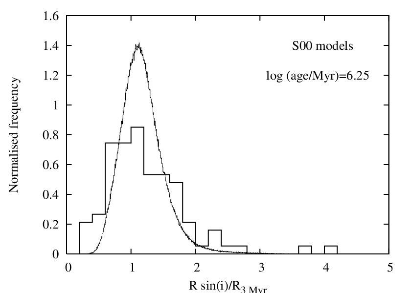
The first distribution of tested was that of a coeval population. The age was specified and then the cumulative distribution of tested against the Monte-Carlo predictions. The assumed age was adjusted to minimise the K-S statistic and select the model distribution least different to the observational data. This process was repeated using both the S00 and DAM97 evolutionary models to calculate . The numerical results are listed in Table 1 and illustrated in Fig 5 (the coeval models are the rows with a dispersion in radius [see section 4.3], set to ). Initially I used Gaussian uncertainties of 150 K and a threshold inclination . The assumed distribution consists of 20 per cent of stars following a uniform distribution for km s-1 with the remaining 80 per cent following an exponential distribution with a decay constant of 12 km s-1 between km s-1. Adopting this, the observed distribution is well reproduced by the model with a K-S rejection probability of per cent (see Jeffries 2007).
For both the DAM97 and S00 models the data are inconsistent with the PMS population being drawn from a single coeval isochrone, at confidence levels of 99.6 and 96.3 per cent respectively. These must be considered lower-limits to the model-rejection confidence level because the mean age was adjusted as a free parameter to minimise the K-S statistic. The “best-fitting” ages are (age/Myr) of 5.88 and 6.25 for the DAM97 and S00 models respectively. These are similar to, but slightly older than, the median ages found from the H-R diagrams in section 2, but note that values determined from the projected radii are independent of the assumed distance to the ONC and unaffected by the binary status of any of the stars.
Fig. 5 shows that the coeval models are too narrow in . Obviously a radius (or age) spread could broaden the model distribution, but so too could a decrease in the assumed value of or an increase in the assumed uncertainties. To test this I ran the coeval S00 models assuming . Table 1 shows the “best-fit” parameters and that the coeval model is still rejected with per cent confidence. Conversely, if were greater than a coeval model would be an even poorer match to the data. I next tried broadening the model distribution by increasing the uncertainty in . The model can still be rejected at per cent confidence unless the uncertainties are approximately doubled to 300 K, which is equivalent to a spectral subclass (1-sigma) uncertainty in the spectral types. Note again that these confidence levels are lower limits because the mean age was tuned to minimise the K-S statistic.
I conclude that unless the uncertainties in spectral classification and have been significantly underestimated by Hillenbrand (1997), then the observed values of are inconsistent with coevality at a reasonably high level of confidence.
4.3 A radius dispersion


Using model 2 (a Gaussian distribution of about a central value defined by a single isochronal age with a standard deviation of ), I simulated a dispersion in radius about an isochronal value. The central isochronal age was again adjusted to minimise the K-S statistic and a range of was tested. The results, using the S00 models to calculate , are listed in Table 1 and illustrated in Fig. 6. If the dispersion increases to then this model can no longer be rejected with per cent confidence. The “best fit” dispersion corresponds to , whilst the model distribution becomes too broad and can be rejected with per cent confidence if . The results using the DAM97 models are similar – models with cannot be rejected with better than 90 per cent confidence – but the required central isochronal age is still smaller ((age/Myr) is 5.88 compared with 6.25 when using the S00 models – see Table 1).
The results above cannot be used to estimate confidence intervals on the best fitting value of , because the central isochronal age has been optimised in each case. The right hand panel of Fig. 6 shows a normalised probability distribution as a function of (calculated using the S00 models), where the probability has been integrated over a wide range of possible mean ages. This illustrates that the best fitting is indeed about 0.15, with 90 per cent of the probability distribution contained between 0.08 and 0.24. The results using the DAM97 models are very similar and give a slightly narrower 90 per cent confidence interval of .
The Monte Carlo models suggest that the observed distribution can be well represented if the observed population has a spread, amounting to a full-width at half maximum of 0.2–0.5 dex, in the stellar radii around an isochronal value. This result is almost independent of which evolutionary models are considered. An obvious interpretation is that this is caused by a spread in ages and this is investigated in the next subsection.
4.4 An age spread


| Gaussian dispersion in log age | ||||||
|---|---|---|---|---|---|---|
| Model | Log central age/Myr | |||||
| (deg) | (dex) | (dex) | ||||
| DAM97 | 30 | 5.85 | 0.48 | 0.059 | 0.886 | 0.31–0.82 |
| DAM97 | 15 | 5.83 | 0.43 | 0.060 | 0.873 | 0.27–0.78 |
| S00 | 30 | 6.22 | 0.36 | 0.045 | 0.989 | 0.20–0.56 |
| S00 | 15 | 6.20 | 0.34 | 0.043 | 0.994 | 0.14–0.54 |
| Exponential age distribution | ||||||
| Model | Log zero point age/Myr | |||||
| (deg) | (Myr) | (Myr) | ||||
| DAM97 | 30 | 4.55 | 1.10 | 0.058 | 0.898 | 0.72–1.30 |
| DAM97 | 15 | 4.95 | 0.95 | 0.057 | 0.911 | 0.58–1.15 |
| S00 | 30 | 5.65 | 1.90 | 0.043 | 0.993 | 1.22–2.82 |
| S00 | 15 | 5.65 | 1.70 | 0.037 | 0.999 | 0.98–2.59 |
Two separate models for an age spread were tested. The first was a Gaussian distribution of age around a central isochrone. The free parameters were the central age and the age dispersion (in logarithmic units), . The second model was an age distribution which is zero up to some starting age, jumps to a maximum and then decays exponentially with a decay constant, , expressed in Myr. This latter model, with a suitably small starting age, represents the exponentially accelerating star formation model advocated by Palla & Stahler (1999). The lowest starting age considered was Myr.
Ages drawn randomly from the Gaussian age distribution were transformed into radii using the appropriate stellar models (at the of each star in the observational dataset) and these radii were perturbed according to the 150 K uncertainties and then subjected to the measurement uncertainties, random axial orientations and selection effects before comparing the observed and modelled distribution of . A grid of models covering a wide range of central ages and age dispersion was calculated for both the DAM97 and S00 models. Assuming that the “correct” solution lay within this grid, I normalised the K-S probabilities and this gave a pair of relative probability grids which are shown in Figs. 7a and 7b. Projection of these grids onto the age dispersion axis gave a best fitting and a confidence interval (analogous to the procedure used to create Fig. 6) which are listed in Table 2. The same procedure was used for the exponential age distribution, with the grid projected onto the axis. The normalised probability grids for this distribution are shown in Figs. 8a and 8b and the numerical results are also listed in Table 2.
There are acceptable fits to the observational data for both Gaussian and exponential age distributions and for both the DAM97 and S00 models. Hence the current data are incapable of distinguishing between these possibilities. As expected, the 90 per cent confidence intervals on and do not encompass zero, which would correspond to a coeval population. The dispersion in age for the Gaussian distribution is quite similar for the DAM97 and S00 models: both models suggest a full-width half maximum spread of factors of a few to and therefore an overall spread in absolute ages that is larger than the central age of the distribution and the median age of the ONC found from the H-R diagram. The exponential distribution has a favoured starting age of essentially zero for the DAM97 models and a decay time scale, of 1.1 Myr. Again this indicates a spread of ages that is larger than the median age of the sample from the H-R diagram. The S00 models favour a non-zero maximum in the age distribution, which is also seen in the H-R diagram-based age distribution shown in Fig. 3, although a very young starting age cannot be ruled out. The decay timescale is about 2 Myr and again this implies a spread of ages that is larger than the median age of the sample.
I ran some more simulations using a smaller value of . The results for these are also given in Table 2. As expected a smaller slightly reduces the age dispersion required to explain the data, but does not affect the broad conclusions. Conversely, a larger would increase the required age dispersion.
4.5 Ages based on the Hertzsprung-Russell diagram

| Model | comment | |||
|---|---|---|---|---|
| (deg) | ||||
| DAM97 | 30 | 0.119 | 0.130 | marginally narrow |
| DAM97 | 15 | 0.089 | 0.430 | good fit |
| S00 | 30 | 0.052 | 0.957 | good fit |
| S00 | 15 | 0.066 | 0.791 | good fit |
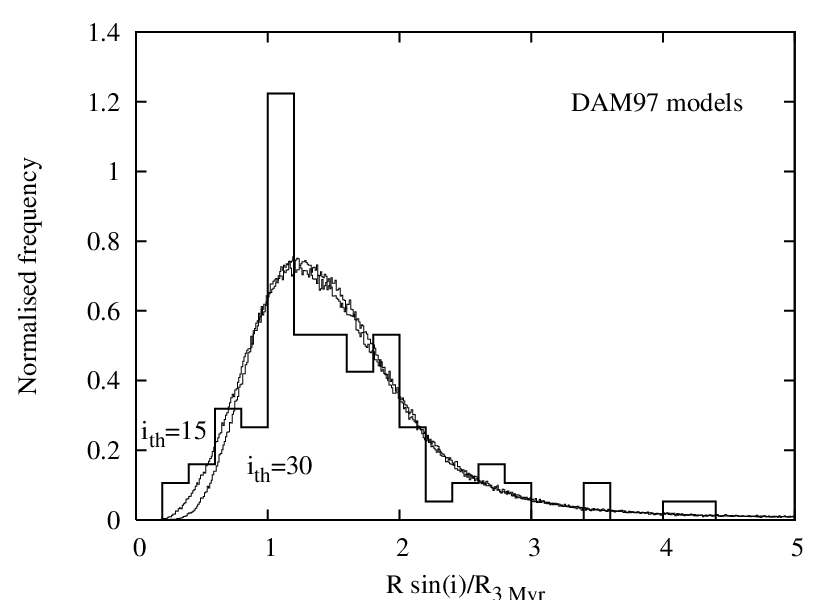
As a final test I constructed age distributions based upon the ages determined from the H-R diagram for the rotation sample, which are shown in the right hand panels of Figs. 2 and 3. These age distributions were used to construct model distributions which in turn were compared with the observed distributions via K-S tests. Initially, was fixed at . A further set of models was generated with to investigate the influence of this parameter.
The comparison between the model and observed distributions of are shown in Fig. 9. Numerical results are listed in Table 3. All of the model distributions are formally compatible with the data and cannot be rejected at the 90 per cent confidence level, although the DAM97 model barely passes this test. Hence the age distributions determined from the Hertzsprung-Russell diagram cannot be discounted as a valid description of the age distribution required by the projected radii. Given the uncertainties in determining ages from the H-R diagram – binarity, accretion, reddening, variability (see Hartmann 2001) – that do not afflict determinations of the projected radii, this might seem somewhat surprising. One might have thought that the age distributions from the H-R diagram would be too broad because of these additional sources of error.
The overall uncertainties in the luminosities have been considered by a number of authors (e.g. Hillenbrand 1997; Hartmann 2001; Rebull et al. 2004), who have concluded that Gaussian uncertainties in luminosity are in the range 0.16–0.20 dex. This leads approximately to Gaussian uncertainties in deduced age of 0.24–0.30 dex for PMS stars (Hartmann 2001). In section 4.4 I found that the age dispersion required to explain the normalised projected radius distribution was probably larger than this. Hence it seems that the uncertainties that affect the H-R diagram-based ages are not large enough to significantly broaden the deduced age distribution beyond that which is indicated by the more robust distribution of projected radii.
5 Discussion
Palla & Stahler (1999) and Huff & Stahler (2006) presented conventional analyses of the ONC H-R diagram, concluding that star formation began at a low level about 10 Myr ago and accelerated up to the present day. Slesnick et al. (2004) also found evidence for an older population in the ONC H-R diagram they assembled, but argued it might be due to younger stars which are viewed in scattered light from circumstellar material. Hartmann (2001) asserted that these large age spreads could be an artefact of observational errors, binarity, variability, differential reddening and accretion luminosity that conspire to cause an observed spread in the H-R diagram that is not due to a significant spread in age. Hartmann (2001) demonstrated that symmetric uncertainties in luminosity can lead to the appearance of an exponentially decaying linear age distribution (see Fig. 2). Palla et al. (2007) support their argument for a true age spread by showing that a few percent of the ONC PMS population show evidence of lithium depletion which is consistent with ages Myr.
The evidence presented in this paper supports the idea that at a given , the ONC stars in our sample do exhibit a spread in radius (and hence luminosity) that is not consistent with isochronal radii at a single age. One interpretation of this is that the ONC stars have a range of ages. Our modelling shows that plausible age distributions can be hypothesised which do explain the observed dispersion in radii. These distributions have spreads in age which are larger than the median age of the sample.
It is worth emphasising that the technique employed here is independent of whether stars have correctly estimated reddening, whether they are accreting, whether their distance is correctly estimated and other sources of uncertainty in calculating their luminosities (see Hillenbrand 1997). The method does depend on reasonable estimates of the measurement uncertainties in and and the assumption that axial orientations are random. The latter assumption is difficult to support or falsify at present (see discussion in Jeffries 2007), although any concentration of inclination angle would require a greater spread of intrinsic radii or ages to match the observed spread in .
A spread in ages is not the only way of explaining a dispersion in radius at a given . For instance Tout, Livio & Bonnell (1999) show that an “age spread” in the H-R diagram could be produced in a coeval population of PMS stars if they have very different accretion histories. Irrespective of whether the spread in radii found here is interpreted in terms of a spread in age, there are important consequences for those using the ONC (and other young star forming regions) to investigate evolutionary trends of angular momentum loss, magnetic activity and circumstellar discs (e.g. Herbst et al. 2005) and for those using evolutionary models to estimate masses and find the (sub)stellar mass function. In these cases, the often-used assumption that stars in a given cluster are close-to-coeval or have similar properties (luminosity, radius) at a given mass or , is not valid.
The sample examined in this paper is subject to a number of limitations. Foremost among these is that I have only been able to comment on the radius distribution of those stars for which periods and measurements are available. Following the discussion in section 2, it is clear that this “rotation sample” is deficient in the small tail of stars which form the controversial elderly population discussed by Palla & Stahler (1999) and Palla et al. (2007).
Whilst the H-R diagram-based age distribution does a reasonable job of reproducing the observed distribution of projected radii, it would be unwise to extrapolate and conclude that the H-R diagram-based ages of the apparently elderly population are reliable. The likely non-Gaussian behaviour of some of the causes of uncertainty in PMS luminosities (e.g. accretion disk scattering or variability) means that this small fraction of outliers could yet be objects whose average intrinsic luminosity has been severely underestimated. Fortunately, the determination of periods is still quite feasible for the fainter ONC members. Large telescopes with multi-object, high resolution spectroscopic capability should then be capable of determining for some fraction of these. Even a small number of values for these objects would be capable of revealing whether they have smaller radii than the rest of the ONC population, as expected from their relative positions in the H-R diagram.
6 Summary
I have taken a sample of PMS objects in the ONC with known rotation periods and projected equatorial velocities, and modelled the resultant distribution of projected equatorial radii with a simple Monte-Carlo simulation. The simulation assumes that rotation axes are randomly oriented in space and takes into account selection effects and observational uncertainties in the data. A comparison between models constructed using a variety of hypotheses concerning the intrinsic distribution of stellar radii leads to the following conclusions.
- 1.
The observed distribution of projected equatorial radii is inconsistent with the hypothesis that the ONC sample is coeval with a high level of confidence. This conclusion can only be weakened if uncertainties in spectral types and inferred effective temperatures are significantly larger than estimated in the original literature sources.
- 2.
A spread in radius (assuming a Gaussian distribution in ) of 0.2–0.5 dex (full width half maximum) about an isochronal locus is required to match the data. This is almost independent of the choice of evolutionary model.
- 3.
If the radius dispersion is modelled in terms of a distribution of ages, then either a Gaussian or exponentially decaying form can feasibly reproduce the data. The absolute values of the median age and age spread or decay timescales depend on which evolutionary models are used, but age spreads must be greater than the median age of the ONC.
- 4.
The age distributions deduced from a conventional H-R diagram adequately reproduce the observed distribution of projected radii, independent of which evolutionary models are used. This suggests that uncertainties in deriving intrinsic luminosities are sufficiently small for the sample considered, that they do not mask the underlying spread in radii and inferred age.
- 5.
The current data are biased in the sense that low-luminosity ONC members, and hence objects that are older in the H-R diagram, are not represented in published catalogues of projected equatorial velocity. This means that the radius and inferred age dispersions found here may be lower limits. In particular, the possibility that some cluster members are Myr older than the bulk of the ONC population cannot be tested. However, given projected equatorial velocities for some of these objects it should easily be possible to check whether these objects have smaller radii consistent with their luminosity-based older ages.
References
- Cohen & Kuhi (1979) Cohen M., Kuhi L. V., 1979, ApJS, 41, 743
- D’Antona & Mazzitelli (1997) D’Antona F., Mazzitelli I., 1997, Mem. Soc. Astr. It., 68, 807
- Hartmann (2001) Hartmann L., 2001, AJ, 121, 1030
- Hartmann et al. (2001) Hartmann L., Ballesteros-Paredes J., Bergin E. A., 2001, ApJ, 562, 852
- Herbst et al. (2002) Herbst W., Bailer-Jones C. A. L., Mundt R., Meisenheimer K., Wackermann R., 2002, A&A, 396, 513
- Herbst & Mundt (2005) Herbst W., Mundt R., 2005, Astrophys. J. , 633, 967
- Hillenbrand (1997) Hillenbrand L. A., 1997, AJ, 113, 1733
- Hillenbrand et al. (1998) Hillenbrand L. A., Strom S. E., Calvet N., Merrill K. M., Gatley I., Makidon R. B., Meyer M. R., Skrutskie M. F., 1998, Astron. J. , 116, 1816
- Huff & Stahler (2006) Huff E. M., Stahler S. W., 2006, ApJ, 644, 355
- Jeffries (2007) Jeffries R. D., 2007, MNRAS, 376, 1109
- Palla et al. (2007) Palla F., Randich S., Pavlenko Y. V., Flaccomio E., Pallavicini R., 2007, ApJ, 659, L41
- Palla & Stahler (1999) Palla F., Stahler S. W., 1999, ApJ, 525, 772
- Palla & Stahler (2000) Palla F., Stahler S. W., 2000, ApJ, 540, 255
- Press et al. (1992) Press W. H., Teukolsky S. A., Vetterling W. T., Flannery B. P., 1992, Numerical Recipes in C: The art of scientific computing, 2nd ed.. Cambridge University Press, Cambridge, UK
- Rebull et al. (2004) Rebull L. M., Wolff S. C., Strom S. E., 2004, AJ, 127, 1029
- Rhode et al. (2001) Rhode K. L., Herbst W., Mathieu R. D., 2001, AJ, 122, 3258
- Sandstrom et al. (2007) Sandstrom K. M., Peek J. E. G., Bower G. C., Bolatto A. D., Plambeck R. L., 2007, ArXiv e-print 0706.2361, 706
- Shu et al. (1987) Shu F. H., Adams F. C., Lizano S., 1987, ARA&A, 25, 23
- Sicilia-Aguilar et al. (2005) Sicilia-Aguilar A., Hartmann L. W., Hernández J., Briceño C., Calvet N., 2005, AJ, 130, 188
- Siess et al. (2000) Siess L., Dufour E., Forestini M., 2000, A&A, 358, 593
- Slesnick et al. (2004) Slesnick C. L., Hillenbrand L. A., Carpenter J. M., 2004, ApJ, 610, 1045
- Tan et al. (2006) Tan J. C., Krumholz M. R., McKee C. F., 2006, ApJ, 641, L121
- Tassis & Mouschovias (2004) Tassis K., Mouschovias T. C., 2004, ApJ, 616, 283
- Tout et al. (1999) Tout C. A., Livio M., Bonnell I. A., 1999, MNRAS, 310, 360
- Vázquez-Semadeni et al. (2005) Vázquez-Semadeni E., Kim J., Shadmehri M., Ballesteros-Paredes J., 2005, ApJ, 618, 344