A Study of the Radiative Decay and Possible Osservation of Direct Photon Emission with the KLOE Detector
Abstract
We present the measurement of the ratio
R = and a first measurement
of the direct emission contribution for the same process.
We use 328 pb-1 of data collected at KLOE in 2001 and 2002, corresponding to about 3
million of events and about 9 thousand radiative events. Our result is
R= for the branching ratio and
for the parameter describing
direct emission.
key words: direct emission
PACS: 13.20.-v, 13.20.Eb
,
,
,
,
,
,
,
,
,
,
,
,
,
,
,
,
,
,
,
,
,
,
,
,
,
,
,
,
,
,
,
,
,
,
,
,
,
,
,
,
,
,
,
,
,
,
,
,
,
,
,
,
,
,
,
,
,
,
,
,
,
,
,
,
,
,
,
,
,
,
,
,
,
,
,
,
,
,
,
,
,
,
1 Corresponding author: Marco Dreucci INFN - LNF, Casella postale 13, 00044 Frascati (Roma), Italy; tel. +39-06-94032696, e-mail marco.dreucci@lnf.infn.it
1 Introduction
The study of radiative decays offers the possibility to obtain informations on the kaon structure and the opportunity to test theories describing hadron interactions and decays, like chiral perturbation theory (ChPT). Two different contribute to the photon emission, inner bremsstrahlung (IB) and direct emission (DE). DE is radiation from intermediate hadronic states and is thus sensitive to hadron structure. In DE is 1% or less of IB which diverges both at 0 and 0 (photon angle w.r.t. lepton). We therefore exclude small angle and energy photon. To compare our result with other measurements we only retain events with and [1]. We define R as
| (1) |
Predictions for R ranges between 0.95 and 0.97 [2]. Recent measurements of R from NA48 and KTeV [3, 4] are in marginal disagreement between each other, so that new measurements are welcome. Following the authors of Ref.[2], in ChPT the structure-dependent (SD) terms are characterized by six amplitude {, }, which in the one-loop approximation are real function, almost constant over phase space. In particular, all relevant SD terms have a similar and simple photon energy spectrum, with a maximum around 100 MeV. This suggests to decompose the photon spectrum in the following manner
| (2) |
in which the different SD contributions are summarized in the so-called distortion function, , which represents the deviation from the pure inner bremmstrahlung. All the information on the structure-dependent terms is contained in the effective strength, , that multiplies . ChPT calculation at order from Ref [2] gives
| (3) |
A first attemp to measure the DE contribution was performed in 2001 by KTeV collaboration
[5], but the uncertainties due to their working hypothesis were too large to infer
definitive conclusions on the parameter.
In our analysis we can isolate DE from IB only because we use both the energy spectrum and
the angular distribution of the radiated photon.
2 The KLOE detector
The KLOE detector consists of a large cylindrical drift chamber (DC), surrounded by a fine grained lead-scintillating fiber electromagnetic calorimeter (EMC). A superconducting coil around the calorimeter provides an axial magnetic field of about 0.52 T.
The drift chamber [6], 4 m in diameter and 3.3 m long, is made of 58 concentric rings of drift cells arranged in a stereo geometry. It is filled with a mixture. The spatial resolutions are 0.15 mm and 2 mm. The transverse momentum resolution is . Two-track vertices are reconstructed with a spatial resolution of 3 mm.
The calorimeter [7] is divided into a barrel and two endcaps. It covers about 98% of the solid angle. It is segmented in depth in five layers, about each. The barrel is divided in 24 sectors, calorimeter cells each, read out by photomultipliers at both ends to measure the arrival time of particles and to reconstruct the space cordinates. Cells close in time and space are grouped into calorimeter clusters. The energy and time resolutions are and , respectively. The spatial resolution are 1.3 cm and 1 cm .
The KLOE trigger [8] uses calorimeter and chamber information. For this analysis, only the calorimeter signals are used. Two energy deposits above threshold ( MeV for the barrel and MeV for the endcaps) are required. Recognition and rejection of cosmic-ray events is also performed at the trigger level. Events with two energy deposits above a 30 MeV threshold in the outermost calorimeter plane are rejected. The 328 pb-1 of data used in this analysis, taken in 2001 and 2002, are divided in 14 periods of about 25 pb-1/period. For each data period we have a corresponding period simulated with Monte Carlo (MC) with about the same statistic.
3 Monte Carlo Generator
In the KLOE MC only radiation from inner bremsstrahlung is described, so we need a Monte Carlo to describe the photon spectrum from direct emission. For this purpose we use a Monte Carlo generator (Kubis generator) based on the code provided by one of the autors of Ref. [2], which implements their calculation. We generate DE events folded with the KLOE reconstruction MC. The accuracy of KLOE Monte Carlo in describing the photon spectrum from IB is at level of 1-2% (an appropriate level for many KLOE measurements). In particular, the KLOE MC generator avoids the problem of the infinite value for the total decay width for a single photon emission by re-summing, in the limit of soft photon energy, the probabilities for multiple photon emission to all order in [9]. Unfortunately, this accuracy level is of the same order of DE contribution, which is 1% of IB one. From a point of view of the measurement of R, this could introduce only a 1% error. On the other side, a fit counting procedure based on a 1%-biased IB distribution could introduce up to 100% error counting in from DE events. For this reason in this analysis we use the Kubis Monte Carlo generator also to describe the photon spectrum from IB.
4 Analysis
The criteria used to select events, briefly summarized below, are the same described in Ref. [10]. Candidate events are tagged by the presence of a decay. Fig. 1 shows that the tagging efficiency, about 66%, is almost independent of the photon energy. The is searched along the direction of its momentum (tagging line), reconstructed from the decay . events are then selected using appropriate kinematical variables of the decay and electron identification by time of flight (TOF).

We have about 3 million of events with a contamination of 7, mainly due to events.
To select events we search for a photon cluster, i.e., a cluster in the calorimeter not assigned to any track. The arrival time of each photon gives an independent determination of the position of the vertex, , the so-called neutral vertex (NV). The method is fully described in Refs. [7] and [11]. The position of the vertex is assumed to be along the line of flight. We require that the distance, , between the position of the neutral vertex and the position of the vertex determined with tracks, to be within 8. In case of more than one photon candidate, we choose the closest to the charged vertex. To evaluate the photon energy we use the charged track momenta and the photon cluster position, . By solving equation 4 below in the hypothesis of neutrino zero mass, we extract the photon energy with a resolution of 1 MeV. This resolution is a factor 10 better than that obtained using the energy deposit information of the calorimeter.
| (4) |
In this equation , , , and are the neutrino, kaon, pion, electron and photon momentum, respectively.
Fig. 2(a) gives the selection efficiency for the signal as taken from Monte Carlo simulation.
 |
 |
| (a) | (b) |
The main background contribution comes from events with an undetected soft-photon to which a cluster from accidentals has been wrongly associated. This background is strongly reduced by requiring 25 MeV and MeV where is the energy of the photon cluster and is the reconstructed photon energy in the laboratory system. This cut is shown in Fig. 2(b). We obtain a factor 10 in background reduction with 6% loss in signal efficiency.
Background from and events after signal selection is at level of 4.2%
and 2.5%, respectively. As shown in Fig. 4, this background overlaps with
the signal of interest DE, so we need to remove it as much as possible.
To remove both and we use a neural network (NN).
To remove events we use a NN based on the photon energy and angle (w.r.t. the lepton),
the track momenta, the missing momentum and , the invariant mass of
photon-neutrino pair.
To remove events we use a NN based on the track momenta, the calorimetric energy
deposit and the cluster centroid position.
Appropriate cuts on the NN output give a background reduction
from 4.2% 0.4% and from 2.5% 1.4%, respectively for and , with
a signal loss of 10%.
To check the data-MC agreement, to calibrate the MC position and correct the
photon selection efficiency we use decay events as a control sample.
These events are selected using a tight kinematical cut in the variable
in the hypothesis of two pion tracks.
Further, we require the presence of a cluster (E60 MeV) not associated to any track,
corresponding to one of the two photons from decay. This high energy photon is used to
tag the presence of the second photon. We select about 350,000 events with a purity of
99.8%.
As a first check of Data-Monte Carlo agreement we compare the energy resolution of the
photons. This can be done because in this control sample we estimate the energy of the second
photon (the tagged photon) exactly in the same way (Eq. 5) than in our signal selection: there we do not detect the neutrino, here we ignore the hard photon (the
tagging photon). Squaring the equation below the (second) photon energy is extracted.
| (5) |
 |
 |
The photon energy resolution is evaluated with respect to a value computed in a
more accurate method using the complete hard photon informations and closing in this way the kinematic.
In Fig. 3(b) the residual is shown for data and Monte Carlo and a good agreement
results.
Further, we use the control sample from to evaluate the distance and its resolution ,
in order to correct and in MC simulation.
Because of the use of to remove accidentals, we also use this control sample
to check the calorimeter energy response. The MC energy response is about 2 MeV lower than data.
To a good approximation, this bias is independent of the energy.
Finally, we evaluate the photon selection efficiency from data and MC in this control sample and use
their ratio to correct photon selection efficiency in MC simulation. The correction is of the order of
a few percent.
5 Fit
In order to count signal events we fit the Monte Carlo spectra to the data ( respectively for IB signal, DE signal, out-of-acceptance ( or ) and physical background from and events). The four distributions used as inputs in the fit are shown in Fig. 4. Actually it is possible to measure R by using the energy spectrum of the photon only (we do it and the result matches), but in this case there is no sensitivity to the presence of a DE term. Only a simultaneous use of the energy and the angle can disentangle the small DE signal.
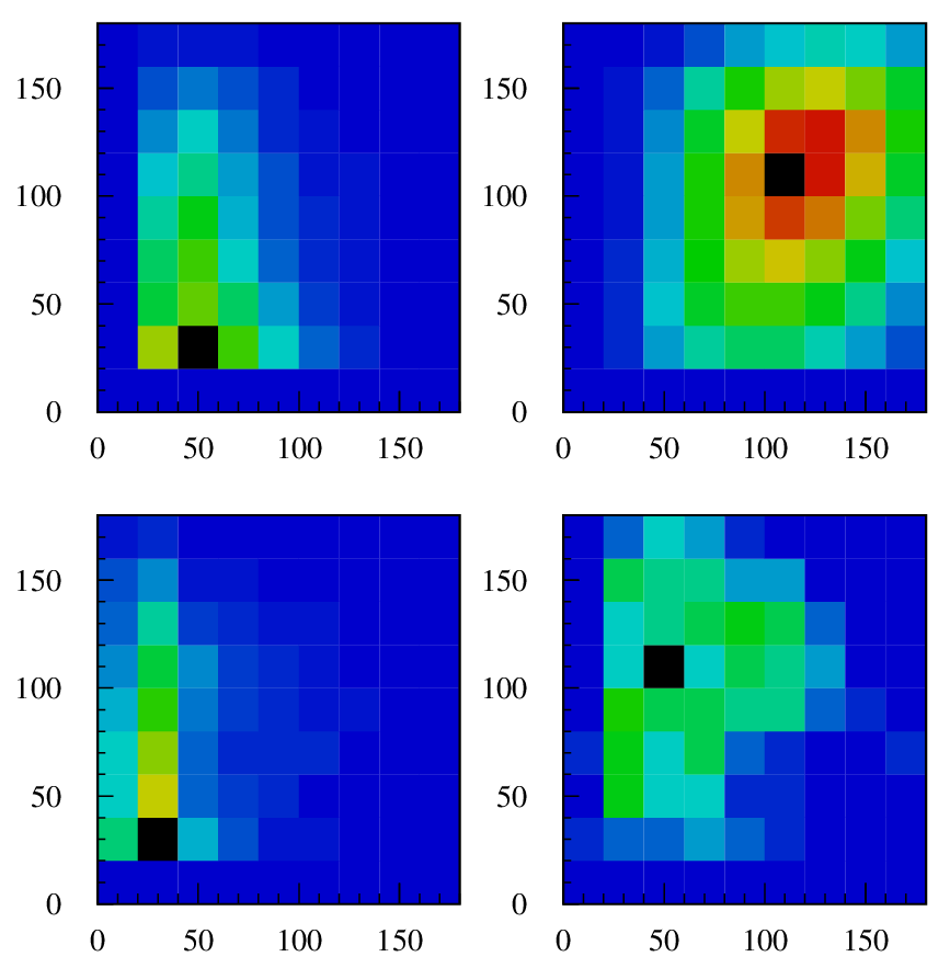
To check the fit stability as a function of run period we fix the background component, otherwise the fit could not converge (too low background statistic) and we do not use the DE shape (no sensitivity in a single run period). The stability is good (). Then we fit all data simultaneously: free parameters of the fit are the population for IB signal, DE signal, -out-of-acceptance. We fix the background contribution of and from MC. As a check we also perform the fit letting all parameters free. The result matches well but there is a loss in statistical accuracy. For this reason the background fraction is not a free parameter of the fit. The result of the fit and the residual are shown in Fig. 5. The two-dimensional MC input shapes are arranged as 8 one dimensional hystograms. Each slice covers 20 degrees, from 20∘ to 180∘.
 |
 |
| (a) | (b) |
The counting result and the correlations of parameters are given, respectively, in Table 1 and Table 2. The is good, giving /dof=60/69).
| Counting result | |||
|---|---|---|---|
| IB signal | -out-acc | DE signal | |
| counting | 9083 | 6726 | -102 |
| error | 213 | 194 | 59 |
| Correlation coefficients | |||
|---|---|---|---|
| Par | 1 | 2 | 3 |
| 1 | 1.000 | -0.586 | -0.254 |
| 2 | 1.000 | -0.022 | |
| 3 | 1.000 | ||
We get the events by counting events after TOF selection, bakground subtraction and efficiency correction. After getting signal from fit counting, taking into account the efficieny and all the efficiency corrections we measure:
| (6) |
Although the for the fit is not bad if we use the KLOE MC to describe the IB spectrum ( probability 55%) the Kubis Monte Carlo is slightly better, giving a 77% probability.
6 Systematic uncertainties
We estimate all the systematics uncertainties by varying the cuts. Tracking, clustering,
track-to-cluster association, NV acceptance and analysis cuts all depends on some parameters
which define our signal. Any variation on these parameters produces a variation on the result.
In the following we list the absolute variation of R.
Tagging.
We tag the requiring that alone satisfies the
calorimeter trigger with the presence of two clusters from associated with fired
trigger sector (autotrigger). We observe a change of 4.
Tracking.
The most effective variable
in the tracking candidates definition is , the distance of closest approach of the track to the
tagging line. We vary by a factor of two. We re-evaluate for each different configuration the
tracking-efficiency correction,which is run-period dependent. The uncertainty on the tracking
efficiency correction is dominated by sample statistics. We observe a change of 1.5.
Clustering.
The most effective variable in the definition of TCA association
is the transverse distance, . We vary the cut on from 15 cm to 30 cm,
corresponding to a change in efficiency of about 17%.
We re-evaluate for each different configuration the clustering efficiency correction, which
is run-period dependent. Also in this case the uncertainty on the clustering efficiency corrections
is dominated by sample statistics.
We observe a change of 5.5 in the result.
Kinematic cuts.
We apply loose kinematic cuts. When varying this cut negligible variation for the results are found.
Tof cut.
Inclusive sample is identified also by using time of flight (TOF). We use a 2-
cut. After varying this cut by 30% we observe a change of 1.3.
Momentum mis-calibration and resolution.
The effect of the momentum scale and the momentum resolution have also been considered.
We conservatively assume a momentum scale uncertainty of 0.1%
We observe a change of 3 for R.
We also investigate the effect of momentum resolution by changing its value of 3%,
corresponding to a worst . The variation on the result is 7.2.
Fiducial volume.
We reduce the fiducial volume by a 20%. This produces a variation of 3.
Rejection of accidentals.
We vary the sliding cut used to remove wrong associations of accidental
cluster (see Fig.2). Varying this cut we have a background variation of a factor of two.
The change in the result is 5.2.
NV acceptance.
We search neutral vertex within a well defined sphere centered around . We vary the
dimension of its radius by a factor of two. We observe a change of 2.9 in the result.
Background.
In a very conservatively way we remove the cut on NN output: in this way the background
level increses almost of a factor of four. We observe a change of 9 for the result.
All systematic errors are summarized in Table 3.
| Source | ||
|---|---|---|
| Tagging | 4.0 | 0.7 |
| Tracking | 1.5 | 0.8 |
| Clustering | 5.5 | 0.1 |
| Kinematic cuts | 0 | 0 |
| TOF-cut | 1.3 | 0.5 |
| p-miscalibration | 3.5 | 0.2 |
| p-resolution | 7.2 | 0.4 |
| Fiducial volume | 3.0 | 0.5 |
| Rejection acc. | 5.2 | 0.4 |
| NV acceptance | 2.9 | 0.3 |
| BKG Reject.by NN | 9.0 | 0.1 |
| Total | 15.5 | 1.4 |
7 Results
Our final result for R is
| (7) |
We also estimate the parameter, defined in the equation 2. Starting from counting result for IB and DE, taking into account the difference in the efficiency (IB efficiency is about 20% higher than DE efficiency), including all systematics we measure
| (8) |
in agreement with evaluation. The systematics on are evaluated as for R. The different contributions are listed in Table 3. The presence of DE contribution reduces the value of R of about 1%. The correlation between R and , including also systematics, is 3.9%.

8 Conclusion
Two different components contribute to the photon emission in events, the inner bremsstrahlung and the direct emission. The latter describes photon radiation from intermediate hadronic states, giving in this way new information on the hadronic structure of kaons. Using and variables KLOE measured the width for for and to the width for inclusive . The DE emission contribution originates from the interference with IB, resulting in a negative effective strength, . KLOE measurement of is the the first attempt to measure direct emission contribution in process. At this stage, the KLOE measurement of R (3% accuracy) is not sufficient to solve the experimental disagreement between NA48 and KTeV measurement.
Acknowledgements
We would like to thank Bastian Kubis, one of the authors of Ref.[2], for the use of his Monte Carlo generator in this analysis. We thank the DAFNE team for their efforts in maintaining low background running conditions and their collaboration during all data-taking. We want to thank our technical staff: G.F.Fortugno for his dedicated work to ensure an efficient operation of the KLOE Computing Center; M.Anelli for his continuous support to the gas system and the safety of the detector; A.Balla, M.Gatta, G.Corradi and G.Papalino for the maintenance of the electronics; M.Santoni, G.Paoluzzi and R.Rosellini for the general support to the detector; C.Piscitelli for his help during major maintenance periods. This work was supported in part by DOE grant DE-FG-02-97ER41027; by EURODAPHNE, contract FMRX-CT98-0169; by the German Federal Ministry of Education and Research (BMBF) contract 06-KA-957; by Graduiertenkolleg ‘H.E. Phys. and Part. Astrophys.’ of Deutsche Forschungsgemeinschaft, Contract No. GK 742; by INTAS, contracts 96-624, 99-37; and by the EU Integrated Infrastructure Initiative HadronPhysics Project under contract number RII3-CT-2004-506078.
References
- [1] M. Doncel, Phys. Lett. B 32 (1970) 623.
- [2] J. Gasser, et al., Eur. Phys. J. C 40 (2005) 205.
- [3] A. Lai, et al., Phys. Lett. B 605 (2005) 247.
- [4] T. Alexopolous, et al., Phys. Rev. D 71 (2005) 0122001.
- [5] A. Alavi-Harati, et al., Phys. Rev. D 64 (2001) 112004.
- [6] M. Adinolfi, et al., The tracking detector of the KLOE experiment, Nucl. Instrum. Meth. A 488 (2002) 51.
- [7] M. Adinolfi, et al., The KLOE electromagnetic calorimeter, Nucl. Instrum. Meth. A 482 (2002) 364.
- [8] M. Adinolfi, et al., The trigger system of the KLOE experiment, Nucl. Instrum. Meth. A 492 (2002) 134.
- [9] C. Gatti, Monte carlo simulation for radiative kaon decays, Eur. Phys. J. C 45 (2006) 417.
- [10] KLOE Collaboration, F. Ambrosino, et al., Phys. Lett. B 636 (2006) 166.
- [11] F. Ambrosino, et al., Data handling, reconstruction, and simulation for the KLOE experiment, Nucl. Instrum. Meth. A 534 (2004) 403.