Effective low-dimensional Hamiltonian for strongly interacting atoms in a transverse trap

Cold atomic gases strongly confined via optical lattice techniques along one or two dimensions and placed in an external magnetic field tuned near a Feshbach resonance provide the exciting possibility to study low-dimensional (low-D) strongly correlated physics in a controllable fashion 1; 2. For weakly interacting atoms in a transverse trap, it is easy to get a low-dimensional Hamiltonian by projecting the atomic wave function to the lowest trap mode. However, the situation gets much more complicated for strongly interacting atoms. It is known that virtual excitation of the transverse trap modes during the atomic collisions could lead to interesting renormalization of the atomic scattering lengths in low dimensions 3; 4; 5. Furthermore, independent of the detuning from the Feshbach resonance, the atoms can always form dimers (two-body bound states) as their ground state configuration in a transverse trap 3; 4; 5; 6; 7; Kestner. Because of the formation of dimers, the problem does not simply reduce to atomic scattering with a renormalized scattering length, but instead, we have to take into account the real population of the atoms in transverse excited levels, which remains significant even for an extremely strong transverse trap Kestner.

In this paper, we construct the low-D (both 1D and 2D) effective Hamiltonian by taking into account the atomic population in the transverse excited modes. To describe the transverse excitations, one can introduce a dressed molecule 8, which is part of the dimer state excluding the atomic population in the lowest transverse level. We observe that for realistic atomic densities, the structure of the dressed molecule is largely fixed by the two-body physics and thus almost density independent. This allows us to derive the renormalized interaction between the atoms and the dressed molecules, which gives the effective many-body Hamiltonian. This effective Hamiltonian reproduces the correct two-body state, and from that, we also fix all the parameters in the Hamiltonian at any detuning of the magnetic field.

We consider an atomic gas free in $D$ dimensions ($D=1,2$) and trapped by a ($3-D$)-dimensional harmonic potential of frequency $\omega$ along the transverse direction. (A single well of the lattice potential can be well approximated with a harmonic trap.) We use the conventional two-channel field theory for Feshbach resonance 9, although one could also use a single-channel approach with an energy-dependent pseudopotential 10. For atoms of mass $m$ possessing internal states $\sigma=\{\uparrow,\downarrow\}$, with contact interactions, the Hamiltonian is

$$H=\sum_{\sigma=\uparrow,\downarrow}\int d^{3}\mathbf{r}\Psi_{\sigma}^{\dagger}\left(-\frac{1}{2}\nabla^{2}+\frac{1}{2}\sum_{i=1}^{3-D}x_{i}^{2}\right)\Psi_{\sigma}\\ +\int d^{3}\mathbf{r}\Phi^{\dagger}\left(-\frac{1}{4}\nabla^{2}+\sum_{i=1}^{3-D}x_{i}^{2}+\nu_{b}\right)\Phi\\ +g_{b}\int d^{3}\mathbf{r}\left(\Psi_{\uparrow}^{\dagger}\Psi_{\downarrow}^{\dagger}\Phi+h.c.\right)+U_{b}\int d^{3}\mathbf{r}\Psi_{\uparrow}^{\dagger}\Psi_{\downarrow}^{\dagger}\Psi_{\downarrow}\Psi_{\uparrow}$$

(1)

where $\Psi\left(\mathbf{r}\right)$ is the atomic field operator and $\Phi\left(\mathbf{r}\right)$ is the molecular field operator. Above, and throughout this paper, we use dimensionless quantities with all energies in units of $\hbar\omega$ and all lengths in units of the trap length scale, $a_{t}=\sqrt{\hbar/m\omega}$. The dimensionless parameters are defined as follows: $\nu_{b}$ is the bare detuning (in units of $\hbar\omega$), $g_{b}$ is the bare atom-molecule coupling rate (in units of $\hbar\omega a_{t}^{3/2}$), and $U_{b}$ is the bare background atomic scattering rate (in units of $\hbar\omega a_{t}^{3}$). The bare parameters are related to the physical ones via the standard renormalization relations:

	$$\displaystyle U_{c}^{-1}=\int\frac{d^{3}\mathbf{k}}{\left(2\pi\right)^{3}}\frac{1}{2E_{\mathbf{k}}}\,,\quad\Gamma^{-1}=1-U_{p}\,U_{c}^{-1},$$
	$$\displaystyle U_{b}=\Gamma U_{p}\,,\quad g_{b}=\Gamma g_{p}\,,\quad\nu_{b}=\nu_{p}+\Gamma g_{p}^{2}U_{c}^{-1}\,,$$		(2)

where the subscript $p$ denotes physical parameters, $E_{\mathbf{k}}\equiv\mathbf{k}^{2}/2$, and the integral is taken in three dimensions with an explicit energy cutoff $E_{c}$ (which finally goes to infinity) imposed on two dimensions, so $U_{c}^{-1}=\sqrt{E_{c}}/2^{3/2}\pi$. The physical parameters $g_{p}$, $U_{p}$, $\nu_{p}$ are determined from the scattering data as $U_{p}=4\pi a_{bg}/a_{t}$, $g_{p}=\sqrt{4\pi\mu_{co}W|a_{bg}|/a_{t}\hbar\omega}$, and $\nu_{p}=\mu_{co}\left(B-B_{0}\right)/\hbar\omega$ ($\mu_{co}$ is the difference in magnetic moments between the two channels), where we have assumed that the s-wave scattering length near resonance has the form $a_{s}=a_{bg}\left(1-\frac{W}{B-B_{0}}\right)$, with $a_{bg}$ as the background scattering length, $W$ as the resonance width, and $B_{0}$ as the resonance point.

Expanding the field operators $\Psi\left(\mathbf{r}\right)$ and $\Phi\left(\mathbf{r}\right)$ in terms of trap eigenmodes in the trapped dimensions and plane waves in the untrapped dimensions yields

$$H=\sum_{\mathbf{mk}\sigma}\left(\epsilon_{\mathbf{k}}+\varepsilon_{\mathbf{m}}\right)a_{\mathbf{mk}\sigma}^{\dagger}a_{\mathbf{mk}\sigma}\\ +\sum_{\mathbf{mk}}\left(\epsilon_{\mathbf{k}}/2+\varepsilon_{\mathbf{m}}+\nu_{b}\right)b_{\mathbf{mk}}^{\dagger}b_{\mathbf{mk}}\\ +\frac{g_{b}}{L^{D/2}}\sum_{\begin{subarray}{c}\mathbf{mnp}\\ \mathbf{kq}\end{subarray}}\gamma_{\mathbf{mnp}}\left(a_{\mathbf{m,k+q,}\uparrow}^{\dagger}a_{\mathbf{n,-k,}\downarrow}^{\dagger}b_{\mathbf{pq}}+\text{h.c.}\right)\\ +\frac{U_{b}}{L^{D}}\sum_{\begin{subarray}{c}\mathbf{mn}\mathbf{m^{\prime}n^{\prime}}\\ \mathbf{kk^{\prime}q}\end{subarray}}\gamma_{\mathbf{mn}}^{\mathbf{m^{\prime}n^{\prime}}}a_{\mathbf{m,k+q,}\uparrow}^{\dagger}a_{\mathbf{n,-k,}\downarrow}^{\dagger}a_{\mathbf{n^{\prime},-k^{\prime},}\downarrow}a_{\mathbf{m^{\prime},k^{\prime}+q,}\uparrow}$$

(3)

where $\mathbf{m}$ indexes trap eigenmodes $\{m_{i}\}$, $i=1,\ldots,3-D$, and $\mathbf{k}$ denotes the wave vector in the untrapped dimensions $\{k_{j}\}$, $j=1,\ldots,D$. The operators $a_{\mathbf{mk}\sigma}$ and $b_{\mathbf{mk}}$ represent the corresponding atomic and Feshbach molecular modes, respectively. The plane wave energy $\epsilon_{\mathbf{k}}$ and the mode energy $\varepsilon_{\mathbf{m}}$ are given by $\epsilon_{\mathbf{k}}=\sum_{j=1}^{D}k_{j}^{2}/2$, $\varepsilon_{\mathbf{m}}=\sum_{i=1}^{3-D}m_{i}$ [for convenience we neglect the constant energy $\left(3-D\right)/2$ in $\varepsilon_{\mathbf{m}}$ as we will measure the two-body bound state energy with respect to the continuum threshold $3-D$]. $L$ is the dimensionless quantization length in the untrapped dimensions. The form factors appearing in Eq. (3) are given by

$$\gamma_{\mathbf{mnp}}=2^{\left(3-D\right)/4}\int d\mathbf{r}\langle\mathbf{m}|\mathbf{r}\rangle\langle\mathbf{n}|\mathbf{r}\rangle\langle\sqrt{2}\mathbf{r}|\mathbf{p}\rangle,$$

(4)

	$\displaystyle\gamma_{\mathbf{mn}}^{\mathbf{m^{\prime}n^{\prime}}}$	$\displaystyle=$	$\displaystyle\int d\mathbf{r}\langle\mathbf{m}|\mathbf{r}\rangle\langle\mathbf{n}|\mathbf{r}\rangle\langle\mathbf{r}|\mathbf{m^{\prime}}\rangle\langle\mathbf{r}|\mathbf{n^{\prime}}\rangle$		(5)
		$\displaystyle=$	$\displaystyle\sum_{\mathbf{p}}\gamma_{\mathbf{mnp}}\gamma_{\mathbf{m^{\prime}n^{\prime}p}}^{\ast},$

with

$$\langle\mathbf{r}|\mathbf{m}\rangle=\prod_{i=1}^{3-D}\frac{e^{-r_{i}^{2}/2}}{\pi^{1/4}\sqrt{2^{m_{i}}m_{i}!}}\;H_{m_{i}}\!\left(r_{i}\right),$$

(6)

where $H_{n}\!\left(x\right)$ is the Hermite polynomial.

The above Hamiltonian is extremely complicated and hard to solve directly. We expect it should reduce to some low-dimensional effective Hamiltonian when the trap confinement is strong enough. In particular, we assume that the many-body energy scale, characterized by the density dependent part of the chemical potential $\mu_{\rho}$, is much less than the trap energy $\hbar\omega$. This is equivalent to assuming that the 1D (or 2D) atomic density $\rho\ll 1$ measured in units of $a_{t}^{-1}$ (or $a_{t}^{-2}$), which is typically the case for realistic systems. Under this condition, when the atoms are far apart, they should stay in the transverse ground level to minimize the energy. The transverse excited levels get populated only when the atoms come close to strongly interact with each other. However, since $\rho\ll 1$ and there is no $n$-particle bound state with $n\geq 3$ for two-component fermions, it is rare for three or more atoms to come close (two atoms can approach each other as there exists a bound dimer state at any detuning $\nu_{p}$ from the Feshbach resonance Kestner). From this argument, we see that the atomic distribution in the transverse excited modes is determined by the short-range physics, where the latter is fixed through the two-body solution. The dimer state of the Hamiltonian $H$ with binding energy (relative to the continuum threshold, $3-D$) $-E_{2B}>0$ and momentum $\mathbf{q}$ can be written in the form $\left|\Psi_{2}\right\rangle=\Psi_{2\mathbf{q}}^{\dagger}\left|0\right\rangle$, where $\left|0\right\rangle$ denotes the vacuum and $\Psi_{2\mathbf{q}}^{\dagger}=\beta b_{\mathbf{0q}}^{\dagger}+\sum_{\mathbf{mnk}}\frac{\eta_{\mathbf{mn}}}{E_{2B}-2\epsilon_{\mathbf{k}}-\epsilon_{\mathbf{q}}/2-\varepsilon_{\mathbf{m}}-\varepsilon_{\mathbf{n}}}a_{\mathbf{m,k+q/2,}\uparrow}^{\dagger}a_{\mathbf{n,-k+q/2,}\downarrow}^{\dagger}$ with the coefficients $\beta$ and $\eta_{\mathbf{mn}}$ given in Ref. Kestner, although the actual expressions are not important for the purposes of this discussion. We thus construct the dressed molecular modes $d_{\mathbf{q}}^{\dagger}$ with the same expression as $\Psi_{2\mathbf{q}}^{\dagger}$, but excluding the $\mathbf{m=n=0}$ term in the summation (correspondingly normalized). These modes $d_{\mathbf{q}}^{\dagger}$ capture the short-range physics and their structure should be basically independent of the atomic density. The coupling between $d_{\mathbf{q}}$ and the atomic modes $a_{\mathbf{0k}\sigma}$ (with a simplified notation as $a_{\mathbf{k}\sigma}$) in the open channel can be approximated with a contact interaction since $d_{\mathbf{q}}$ is tightly confined in space to a volume on the order of $a_{t}^{3}$ in the deep BCS regime and even smaller in the crossover and BEC regimes Kestner. The general effective Hamiltonian for $d_{\mathbf{q}}$ and $a_{\mathbf{k}\sigma}$ then takes the form

$$H_{\text{eff}}=\sum_{\mathbf{k}\sigma}\epsilon_{\mathbf{k}}a_{\mathbf{k}\sigma}^{\dagger}a_{\mathbf{k}\sigma}+\sum_{\mathbf{q}}\left(\epsilon_{\mathbf{q}}/2+\lambda_{b}\right)d_{\mathbf{q}}^{\dagger}d_{\mathbf{q}}\\ +\frac{\alpha_{b}}{L^{D/2}}\sum_{\mathbf{kq}}\left(a_{\mathbf{k+\frac{q}{2},}\uparrow}^{\dagger}a_{\mathbf{-k+\frac{q}{2},}\uparrow}^{\dagger}d_{\mathbf{q}}+\text{h.c.}\right)\\ +\frac{V_{b}}{L^{D}}\sum_{\mathbf{kk^{\prime}q}}a_{\mathbf{k+\frac{q}{2},}\uparrow}^{\dagger}a_{\mathbf{-k+\frac{q}{2},}\downarrow}^{\dagger}a_{\mathbf{-k^{\prime}+\frac{q}{2},}\downarrow}a_{\mathbf{k^{\prime}+\frac{q}{2},}\uparrow}$$

(7)

where $\lambda_{b}$ (in units of $\hbar\omega$) is the relative detuning , $\alpha_{b}$ (in units of $\hbar\omega a_{t}^{D/2}$) is the coupling rate, and $V_{b}$ (in units of $\hbar\omega a_{t}^{D}$) represents the remaining background interaction in the open channel. We introduce the physical parameters related to three bare parameters in $H_{\text{eff}}$ via a low-D renormalization analogous to Eq. (2):

	$$\displaystyle V_{c}^{-1}=\int\frac{d^{D}\mathbf{k}}{\left(2\pi\right)^{D}}\frac{1}{2\epsilon_{\mathbf{k}}+3-D}\,,\quad\Omega^{-1}=1-V_{p}V_{c}^{-1},$$
	$$\displaystyle V_{p}=\Omega^{-1}V_{b}\,,\quad\alpha_{p}=\Omega^{-1}\alpha_{b}\,,\quad\lambda_{p}=\lambda_{b}-\Omega\alpha_{p}^{2}V_{c}^{-1}\,.$$		(8)

Note that the zero-point energy $3-D$ appears explicitly in the definition of $V_{c}^{-1}$, otherwise there is an artificial infrared divergence. These definitions of the physical parameters are justified as we will see below that they remove exactly the ultraviolet divergence associated with the contact interaction.

The effective Hamiltonian $H_{\text{eff}}$ should reproduce the same physics represented by the 3D Hamiltonian $H$ when the system is near the ground state with the energy per particle close to $E_{2B}/2$ (as $\mu_{\rho}\ll 1$ in units of $\hbar\omega$). To determine the parameters in $H_{\text{eff}}$, we match the exact two-body bound state obtained from the original $H$. Specifically, we first determine the effective background scattering $V_{p}$ by matching the bound state physics in the deep BCS limit, where the population is entirely atoms in the lowest trap mode. Then, for general detuning, matching the binding energy and the bound state gives two constraints which determine the remaining parameters, $\lambda_{b}$ and $\alpha_{b}$. Since the composition of the dressed molecule $d_{\mathbf{q}}$ is a function of detuning $\nu_{p}$, or equivalently, of the 3D scattering length, so are these two parameters.

All the two-body physics contained in a given Hamiltonian are embodied in its T-matrix, defined by $T\!\left(E\right)=H_{I}+H_{I}G\!\left(E\right)H_{I}=H_{I}+H_{I}G_{0}\!\left(E\right)T\!\left(E\right)$, where $H_{I}$ is the interaction part of the Hamiltonian $H$, $G\!\left(E\right)=(E-H)^{-1}$ is the full two-body propagator, and $G_{0}\!\left(E\right)=(E-H_{0})^{-1}$ is the free two-body propagator. Physically, the matrix element $\langle\mathbf{2}|T\left(E\right)|\mathbf{1}\rangle$ is the sum of the direct process whereby a pair of atoms scatters from state $|\mathbf{1}\rangle$ to state $|\mathbf{2}\rangle$ and the indirect processes whereby the atoms scatter into an intermediate state, propagate with energy $E$, and then scatter into the final state. From its definition, it is clear that the T-matrix has simple poles where $E$ is equal to a two-body bound state of the Hamiltonian. Furthermore, the residue of the diagonal matrix element $\langle\mathbf{1}|T\left(E\right)|\mathbf{1}\rangle$ at such a pole, $E=E_{n}$, is $|\langle\mathbf{1}|H_{I}|\Psi_{n}\rangle|^{2}=|\langle\mathbf{1}|H-H_{0}|\Psi_{n}\rangle|^{2}=\left(E_{n}-\epsilon_{\mathbf{1}}\right)^{2}|\langle\mathbf{1}|\Psi_{n}\rangle|^{2}$, where $\epsilon_{\mathbf{1}}$ is the noninteracting energy of state $|\mathbf{1}\rangle$. Thus, the residue of a given diagonal matrix element determines the fraction of the bound state in the given basis state. We shall use both of these facts in matching the two-body bound state properties of the exact and effective Hamiltonians.

In the appendix, we derive the general two-body T-matrix associated with the Hamiltonian $H$ in Eq. (3). For a pair of atoms asymptotically in the lowest mode of the trap, the corresponding diagonal T-matrix element (in units of $a_{t}^{D}\hbar\omega$) as a function of the two-body energy $E$ (measured with respect to the continuum threshold, $3-D$) is

$$\left[T\left(E\right)\right]^{-1}=\gamma_{\mathbf{000}}^{-2}\left(\left[U_{p}^{\text{eff}}\left(E\right)\right]^{-1}-S_{p}\left(E\right)\right)\,,$$

(9)

where $\gamma_{\mathbf{000}}=\left(2\pi\right)^{\left(D-3\right)/4}$, $U_{p}^{\text{eff}}\left(E\right)\equiv U_{p}-g_{p}^{2}/(\nu_{p}-E)$ and, from the normalization in Eq. (2), $U_{p}^{\text{eff}}\left(E\right)=U_{b}^{\text{eff}}\left(E\right)+U_{c}^{-1}\equiv U_{b}-g_{b}^{2}/\left(\nu_{b}-E\right)+U_{c}^{-1}$, and the function

$$S_{p}\left(E\right)\equiv\frac{1}{L^{D}}\sum_{\mathbf{mnk}}\frac{\gamma_{\mathbf{mn0}}^{2}}{E-2\epsilon_{\mathbf{k}}-\varepsilon_{\mathbf{m}}-\varepsilon_{\mathbf{n}}}+U_{c}^{-1}\\ =\frac{-1}{2^{5/2}\pi}\begin{cases}\zeta\left(1/2,-E/2\right)&\text{{\small{\emph{D}=1}}}\\ \int_{0}^{\infty}ds\left[\frac{\Gamma\left(s-E/2\right)}{\Gamma\left(s+1/2-E/2\right)}-\frac{1}{\sqrt{s}}\right]&\text{{\small{\emph{D}=2}}}\end{cases}$$

(10)

sum note. In the above we have used the gamma function $\Gamma\left(x\right)$ and the Hurwitz zeta function $\zeta\left(s,x\right)=\lim_{N\rightarrow\infty}\sum_{n=0}^{N}\left(n+x\right)^{-s}-\left(N+x\right)^{1-s}/(1-s)$.

The two-body bound state corresponds to a pole of the T-matrix element above with $\left[T\left(E_{2B}\right)\right]^{-1}=0$ at the binding energy $\left|E_{2B}\right|$, which gives the eigen-equation

$$\left[U_{p}^{\text{eff}}\left(E_{2B}\right)\right]^{-1}=S_{p}\left(E_{2B}\right)$$

(11)

to determine $E_{2B}$. Also, as discussed above, the atom pair population of the lowest trap mode is determined by the residue of the above T-matrix element at this pole. Since the bound state of the effective Hamiltonian comprises only atom pairs in the lowest trap mode and dressed molecules, specifying the population in the lowest mode is sufficient, in conjunction with normalization, to determine the entire bound state of $H_{\text{eff}}$. Thus, to ensure that the effective and the exact Hamiltonians produce the same two-body bound state, we just need to obtain $\left[T\left(E\right)\right]^{-1}$ from both $H$ and $H_{\text{eff}}$, and require them to match to first order in $E-E_{2B}$.

Following the same approach as in the Appendix, the corresponding T-matrix element from the effective Hamiltonian $H_{\text{eff}}$ is obtained as

$$\left[T^{\text{eff}}\left(E\right)\right]^{-1}=\left[V_{p}^{\text{eff}}\left(E\right)\right]^{-1}-\gamma_{\mathbf{000}}^{-2}\sigma_{p}\left(E\right),$$

(12)

where $\left[V_{p}^{\text{eff}}\left(E\right)\right]^{-1}\equiv\left[V_{p}-\alpha_{p}^{2}/\left(\lambda_{p}-E\right)\right]^{-1}=\left[V_{b}-\alpha_{b}^{2}/\left(\lambda_{b}-E\right)\right]^{-1}+V_{c}^{-1}$, and the function

	$\displaystyle\sigma_{p}\left(E\right)$	$\displaystyle\equiv\gamma_{\mathbf{000}}^{2}\int\frac{d^{D}\mathbf{k}}{\left(2\pi\right)^{D}}\left[\frac{1}{E-2\epsilon_{\mathbf{k}}}+\frac{1}{2\epsilon_{\mathbf{k}}+3-D}\right]$
		$\displaystyle=\begin{cases}\frac{-1}{4\pi\sqrt{-E}}+\frac{1}{2^{5/2}\pi}&D=1\\ \frac{\ln\left(-E\right)}{2^{5/2}\pi^{3/2}}&D=2\end{cases}$		(13)

We require the effective background term alone to reproduce the two-body physics on the deep BCS side, where the dressed molecule population is negligible. Matching Eqs. (9) and (12) in that region yields

$$V_{p}^{-1}=\left(2\pi\right)^{\left(3-D\right)/2}\left(U_{p}^{-1}-C_{p}\right)$$

(14)

where $C_{p}\equiv\lim_{\nu_{p}\rightarrow\infty}S_{p}\left(E_{2B}\right)-\sigma_{p}\left(E_{2B}\right)$. In this way, we obtain an effective single-channel model on the deep BCS side which recovers the low-energy scattering models of Refs. 3; 4; 7. However, the single-channel model with a renormalized scattering length $\left(\propto V_{p}\right)$ is not adequate near resonance or on the BEC side where the dressed molecule population becomes significant.

To fix the parameters $\lambda_{p}$ and $\alpha_{p}$, we compare the T-matrix in Eqs. (9) and (12) at general detuning, and require them to match for the zeroth and the first orders in expansion with $\left(E-E_{2B}\right)$ (which are responsible for reproducing the same binding energy and the bound state, respectively). After some algebra, we obtain

	$$\displaystyle\lambda_{p}=E_{2B}\!-\!\frac{\sigma_{p}\left(E_{2B}\right)}{\partial_{E_{2B}}\left[U_{p}^{\text{eff}-1}-\left(S_{p}-\sigma_{p}\right)\right]}\left[1-\frac{\sigma_{p}\left(E_{2B}\right)}{U_{p}^{-1}-C_{p}}\right]$$		(15)
	$$\displaystyle\alpha_{p}^{2}=\frac{\left(2\pi\right)^{\left(D-3\right)/2}}{\partial_{E_{2B}}\left[U_{p}^{\text{eff}-1}-\left(S_{p}-\sigma_{p}\right)\right]}\left[1-\frac{\sigma_{p}\left(E_{2B}\right)}{U_{p}^{-1}-C_{p}}\right]^{2}$$		(16)

where $\partial_{E_{2B}}$ means $\partial/\partial E\big|_{E=E_{2B}}$. Since the derivative of Eq. (10) is not obvious, we write it below explicitly dS note.

$$\partial_{E_{2B}}S_{p}=\frac{-1}{2^{7/2}\pi}\begin{cases}\frac{1}{2}\zeta\left(3/2,-E_{2B}/2\right)&D=1\\ \frac{\Gamma\left(-E_{2B}/2\right)}{\Gamma\left(1/2-E_{2B}/2\right)}&D=2\end{cases}$$

(17)

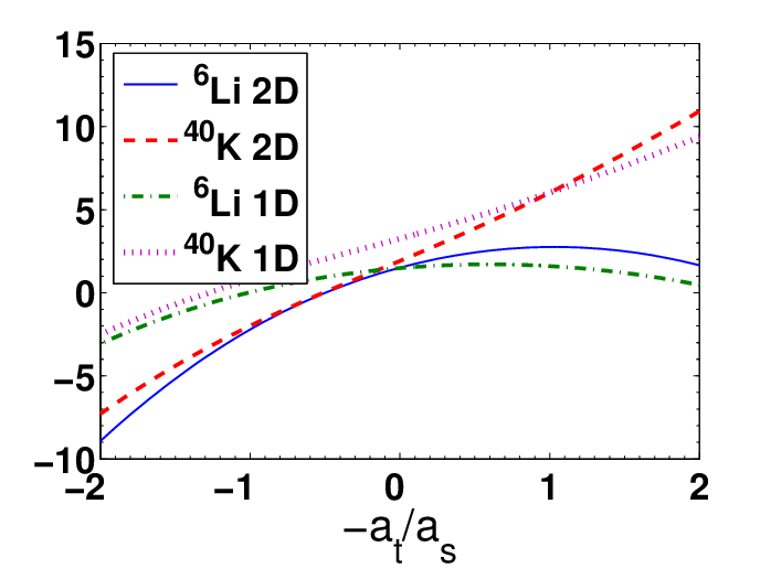
Thus, Eqs. (14, 15, 16) along with the low-D renormalization procedure in Eq. (8) fix the parameters of the effective Hamiltonian as functions of the two-body binding energy, $E_{2B}$, which is connected to the physical detuning $\nu_{p}$ through Eq. (11). The detuning-dependent parameters are plotted in Fig. 1 across resonance, assuming the same typical 3D parameters as in Ref. Kestner. The difference in the sign of $U_{p}$ between ⁶Li and ⁴⁰K gives rise to quite different looking effective parameters. However, the relevant combination of parameters for mean-field calculations, $V_{p}^{\text{eff}}$, is very nearly universal. We plot $V_{p}^{\text{eff}}\left(2\mu\right)$ across resonance with $\mu=E_{2B}/2+\mu_{\rho}$ for small values of $\mu_{\rho}$ ($\mu$ has the meaning of the total chemical potential including the per-particle binding energy $E_{2B}/2$). The slight difference between the ⁶Li and ⁴⁰K curves stems from the slight difference in binding energies as a function of the 3D scattering length. In the low density limit $\mu_{\rho}\rightarrow 0$, $V_{p}^{\text{eff}}$ can approach infinity in 2D on the BEC side where $\lambda_{p}=E_{2B}$, but in 1D $V_{p}^{\text{eff}}$ is always attractive since we have $\lambda_{p}>E_{2B}$ at any detuning. The 2D resonance-like behavior ($V_{p}^{\text{eff }}\left(E\right)\rightarrow\infty$) around energy $E\sim E_{2B}$ should not be confused, however, with the confinement induced resonance discussed in Ref. 3 around energy $E\sim 0$. Due to the existence of the two-body bound state with $E_{2B}<0$, the resonance discussed in 3 is not for the ground-state configuration of the system. Moreover, the relevant quantity for a typical many-body calculation is $1/V_{p}^{\text{eff}}\left(E\right)$, which is continuous.

In summary, we have derived an effective low-dimensional Hamiltonian for strongly interacting atomic gas trapped in one or two dimensions and free in the other dimensions. Excited trap modes are important to the bound state physics, requiring the effective parameters to assume a highly nontrivial magnetic field dependence. All the parameters in the Hamiltonian have been fixed from two-body considerations. This effective Hamiltonian can provide a starting point to understand the low-dimensional many-body physics when the system is near its ground state configuration (with the chemical potential close to the per-particle binding energy $E_{2B}/2$).

This work was supported by the MURI, the DARPA, the NSF award (0431476), the DTO under ARO contracts, and the A. P. Sloan Foundation. J.P.K. gratefully acknowledges many helpful discussions with Wei Zhang and G.-D. Lin.

Below we derive the center-of-mass two-body T-matrix between atoms in arbitrary trap modes from the 3D Hamiltonian $H$ in Eq. (1). We use $|\mathbf{mnk}\rangle$ to denote an atomic pair state in trap modes $\mathbf{m}$ and $\mathbf{n}$ having relative momentum $\mathbf{k}$, and $|\mathbf{p}\rangle$ to denote a molecule in trap mode $\mathbf{p}$. With the definition $T=H_{I}+H_{I}G_{0}T$, we evaluate the propagator at energy $E$ and obtain

$$\langle\mathbf{mnk}|T|\mathbf{m^{\prime}n^{\prime}k^{\prime}}\rangle=U_{b}\gamma_{\mathbf{mn}}^{\mathbf{m^{\prime}n^{\prime}}}\!+\sum_{\mathbf{p}}\frac{g_{b}\gamma_{\mathbf{mnp}}\langle\mathbf{p}|T|\mathbf{m^{\prime}n^{\prime}k^{\prime}}\rangle}{E-\varepsilon_{\mathbf{p}}-\nu_{b}}\\ +\sum_{\mathbf{m^{\prime\prime}n^{\prime\prime}k^{\prime\prime}}}\frac{U_{b}\gamma_{\mathbf{mn}}^{\mathbf{m^{\prime\prime}n^{\prime\prime}}}\langle\mathbf{m^{\prime\prime}n^{\prime\prime}k^{\prime\prime}}|T|\mathbf{m^{\prime}n^{\prime}k^{\prime}}\rangle}{E-2\epsilon_{\mathbf{k^{\prime\prime}}}-\varepsilon_{\mathbf{m^{\prime\prime}}}-\varepsilon_{\mathbf{n^{\prime\prime}}}}$$

(18)

$$\langle\mathbf{p}|T|\mathbf{mnk}\rangle=g_{b}\gamma_{\mathbf{mnp}}+\!\!\!\!\!\sum_{\mathbf{m^{\prime\prime}n^{\prime\prime}k^{\prime\prime}}}\!\!\!\!\frac{g_{b}\gamma_{\mathbf{m^{\prime\prime}n^{\prime\prime}p}}\langle\mathbf{m^{\prime\prime}n^{\prime\prime}k^{\prime\prime}}|T|\mathbf{mnk}\rangle}{E-2\epsilon_{\mathbf{k^{\prime\prime}}}-\varepsilon_{\mathbf{m^{\prime\prime}}}-\varepsilon_{\mathbf{n^{\prime\prime}}}}$$

(19)

Substituting Eq. (19) into Eq. (18), we get

$$\langle\mathbf{mnk}|T|\mathbf{m^{\prime}n^{\prime}k^{\prime}}\rangle=\sum_{\mathbf{p}}U_{b}^{\text{eff}}\left(E-\varepsilon_{\mathbf{p}}\right)\gamma_{\mathbf{mnp}}\biggl[\gamma_{\mathbf{m^{\prime}n^{\prime}p}}\\ +\sum_{\mathbf{m^{\prime\prime}n^{\prime\prime}k^{\prime\prime}}}\frac{\gamma_{\mathbf{m^{\prime\prime}n^{\prime\prime}p}}}{E-2\epsilon_{\mathbf{k^{\prime\prime}}}-\varepsilon_{\mathbf{m^{\prime\prime}}}-\varepsilon_{\mathbf{n^{\prime\prime}}}}\langle\mathbf{m^{\prime\prime}n^{\prime\prime}k^{\prime\prime}}|T|\mathbf{m^{\prime}n^{\prime}k^{\prime}}\rangle\biggr]$$

(20)

where $U_{b}^{\text{eff}}\left(E\right)$ is defined in the text. Note that we can separate out the final state dependence

$$\langle\mathbf{mnk}|T|\mathbf{m^{\prime}n^{\prime}k^{\prime}}\rangle=\sum_{\mathbf{p}}U_{b}^{\text{eff}}\left(E-\varepsilon_{\mathbf{p}}\right)\gamma_{\mathbf{mnp}}\tilde{T}_{\mathbf{m^{\prime}n^{\prime}k^{\prime}}}^{\mathbf{p}}$$

(21)

Substituting this form into Eq. (20), we get

$$\tilde{T}_{\mathbf{m^{\prime}n^{\prime}k^{\prime}}}^{\mathbf{p}}=\gamma_{\mathbf{m^{\prime}n^{\prime}p}}+\sum_{\mathbf{p^{\prime}}}U_{b}^{\text{eff}}\left(E-\varepsilon_{\mathbf{p^{\prime}}}\right)\tilde{T}_{\mathbf{m^{\prime}n^{\prime}k^{\prime}}}^{\mathbf{p^{\prime}}}\\ \times\sum_{\mathbf{m^{\prime\prime}n^{\prime\prime}k^{\prime\prime}}}\frac{\gamma_{\mathbf{m^{\prime\prime}n^{\prime\prime}p}}\gamma_{\mathbf{m^{\prime\prime}n^{\prime\prime}p^{\prime}}}}{E-2\epsilon_{\mathbf{k^{\prime\prime}}}-\varepsilon_{\mathbf{m^{\prime\prime}}}-\varepsilon_{\mathbf{n^{\prime\prime}}}}$$

(22)

The inner sum is equal to $S\left(E-\varepsilon_{\mathbf{p}}\right)\delta_{\mathbf{p^{\prime}}\mathbf{p}}$ sum note, where $S\left(E\right)\equiv S_{p}\left(E\right)-U_{c}^{-1}$ and $S_{p}\left(E\right)$ is defined as in Eq. (10), so we can solve Eq. (22) to obtain

$$\tilde{T}_{\mathbf{m^{\prime}n^{\prime}k^{\prime}}}^{\mathbf{p}}=\frac{\gamma_{\mathbf{m^{\prime}n^{\prime}p}}}{1-U_{b}^{\text{eff}}\left(E-\varepsilon_{\mathbf{p}}\right)S\left(E-\varepsilon_{\mathbf{p}}\right)}$$

(23)

and

$$\langle\mathbf{mnk}|T|\mathbf{m^{\prime}n^{\prime}k^{\prime}}\rangle=\sum_{\mathbf{p}}\frac{\gamma_{\mathbf{mnp}}\gamma_{\mathbf{m^{\prime}n^{\prime}p}}}{\left[U_{p}^{\text{eff}}\left(E-\varepsilon_{\mathbf{p}}\right)\right]^{-1}-S_{p}\left(E-\varepsilon_{\mathbf{p}}\right)}$$

(24)

$$\langle\mathbf{p}|T|\mathbf{mnk}\rangle=\frac{g_{b}\gamma_{\mathbf{mnp}}}{1-U_{b}^{\text{eff}}\left(E-\varepsilon_{\mathbf{p}}\right)S\left(E-\varepsilon_{\mathbf{p}}\right)}$$

(25)

For the special case of atoms asymptotically in the lowest mode of the trap, $\mathbf{m}=\mathbf{n}=\mathbf{m^{\prime}}=\mathbf{n^{\prime}}=\mathbf{0}$, we use the fact that $\gamma_{\mathbf{00p}}\propto\delta_{\mathbf{p},\mathbf{0}}$ to obtain Eq. (9) from Eq. (24).

References

- (1) H. Moritz, T. Stöferle, K. Günter, M. Köhl, and T. Esslinger, Phys. Rev. Lett. 94, 210401 (2005); T. Stöferle, H. Moritz, K. Günter, M. Köhl, and T. Esslinger, ibid. 96, 030401 (2006); J. K. Chin, D. E. Miller, Y. Liu, C. Stan, W. Setiawan, C. Sanner, K. Xu, and W. Ketterle, Nature (London) 443, 961 (2006).
- (2) B. Paredes et al., Nature 429, 277 (2004); T. Kinoshita, T. Wenger, and D. Weiss, Science 305, 5687 (2004); Z. Hadzibabic, P. Kruger, M. Cheneau, B. Battelier, and J. Dalibard, Nature 441,1118 (2006).
- (3) M. Olshanii, Phys. Rev. Lett. 81, 938 (1998); T. Bergeman, M. G. Moore, M. Olshanii, Phys. Rev. Lett. 91, 163201 (2003).
- (4) D.S. Petrov, M. Holzmann, and G.V. Shlyapnikov, Phys. Rev. Lett 84, 2551 (2000); D.S. Petrov and G.V. Shlyapnikov, Phys. Rev. A 64, 012706 (2001).
- (5) E.L. Bolda, E. Tiesinga, and P.S. Julienne, Phys. Rev. A 68, 032702 (2003).
- (6) T. Busch, B. G. Englert, K. Rzazewski, and M. Wilkens, Found. Physics 28, 549 (1998).
- (7) V.A. Yurovsky, Phys. Rev. A 73, 052709 (2006).
- (8) J.P. Kestner and L.-M. Duan, Phys. Rev. A 74, 053606 (2006).
- (9) L.-M. Duan, Phys. Rev. Lett. 95, 243202 (2005); arXiv:0706.2161.
- (10) M. Holland, S.J.J.M.F Kokkelmans, M.L. Chiofalo, and R. Walser, Phys. Rev. Lett. 87, 120406 (2001); E. Timmermans, P. Tommasini, M. Hussein, and A. Kerman, Phys. Rep. 315, 199 (1999).
- (11) D. Blume and C.H. Greene, Phys. Rev. A 65, 043613 (2002).
- (12) We first differentiate the summand in Eq. (10), then sum.
- (13) Rewriting the numerator with the explicit definitions (4) and (6) and using the identity , valid for , to rewrite the denominator, the sum can be written as a []-dimensional integral of a more convenient sum which can be done analytically using Mehler’s Hermite polynomial formula. The spatial integrals can then be performed, giving rise to the Kronecker delta. Finally, after integrating over the dummy variable , the results can be analytically continued to .