In two recent papers [1], Georgi has proposed to look seriously at the possibility that a conformal sector with a non-trivial fixed point might be realized in nature and couple to our standard world of particles. He has shown how such sector would have very unconventional features and, at least in the appropriate energy range, will behave unlike a common particle sector. These two seminal papers have been followed by a deluge of work [2, 3] in all sorts of phenomenological implications that such an unparticle sector could have.

In this paper we consider how unparticles could affect one of the central issues of contemporary particle physics: the breaking of the electroweak symmetry and the nature of the Higgs sector. After a brief reminder of some aspects of unparticles relevant for this discussion we show in section 2 how unparticles, if coupled to the Higgs operator $|H|^{2}$ as recently considered in [4], can have a dramatic impact on electroweak symmetry breaking already at tree-level. In section 3 we study the mixed unparticle-Higgs propagator and spectral function and show: i) How unparticles can shift the Higgs mass away from its Standard Model (SM) value, $2\lambda v^{2}$, and, conversely; ii) How electroweak symmetry breaking affects the unparticle sector by breaking its conformal symmetry and generating a mass gap. For Higgs masses above that gap we also show that unparticles can also affect significantly the Higgs width.

We will consider the ultraviolet (UV) coupling of an operator of dimension $d_{UV}$ in the unparticle sector to the SM dimension-two operator $|H|^{2}$ as

$\displaystyle\mathcal{L}=-\frac{1}{\mathcal{M}_{U}^{d_{UV}-2}}|H|^{2}\mathcal{O}_{UV}\ ,$

(1.1)

which flows in the infrared (IR) to

$\displaystyle\mathcal{L}=-C_{U}\left(\frac{\Lambda_{U}}{\mathcal{M}_{U}}\right)^{d_{UV}-2}\Lambda_{U}^{2-d_{U}}|H|^{2}\mathcal{O}_{U}\equiv-\kappa_{U}|H|^{2}\mathcal{O}_{U}\ ,$

(1.2)

where $d_{U}$ is the scaling dimension of the unparticle operator $\mathcal{O}_{U}$ (usually considered in the interval $1<d_{U}<2$), $C_{U}$ is a dimensionless constant (whose value can be absorbed in the definition of the scales $\Lambda_{U}$ and $\mathcal{M}_{U}$ and so it will be fixed to one) and $\kappa_{U}$ has mass dimension $2-d_{U}$.

We take the tree-level Higgs potential

$\displaystyle V_{0}=m^{2}|H|^{2}+\lambda|H|^{4}\ ,$

(1.3)

where the squared mass parameter can have either sign or even vanish and the quartic coupling $\lambda$ is related in the SM to the Higgs mass at tree level by $m_{h0}^{2}=2\lambda v^{2}$ (for $m^{2}<0$). We write the Higgs real direction as $Re(H^{0})=(h^{0}+v)/\sqrt{2}$, with $v=246$ GeV.

The unparticle operator $\mathcal{O}_{U}$ coupled to $|H|^{2}$ in Eq. (1.2) has spin zero and its propagator is [1, 2]

$\displaystyle P_{U}(p^{2})=\frac{A_{d_{U}}}{2\sin(\pi d_{U})}\frac{i}{(-p^{2}-i\epsilon)^{2-d_{U}}},\quad A_{d_{U}}\equiv\frac{16\pi^{5/2}}{(2\pi)^{2d_{U}}}\frac{\Gamma(d_{U}+1/2)}{\Gamma(d_{U}-1)\Gamma(2d_{U})}\ .$

(1.4)

The spectral function representation for this propagator

$\displaystyle-iP_{U}(p^{2})=\int_{0}^{\infty}\frac{\rho_{U}(s)}{p^{2}-s+i\epsilon}\ ds\ ,$

(1.5)

gives

$\displaystyle\rho_{U}(s)=\frac{A_{d_{U}}}{2\pi}s^{d_{U}-2}\ ,$

(1.6)

with no poles and an essential singularity at $s=0$.

We are interested in the possible effects of the unparticle sector on the Higgs sector through the coupling (1.2) and, in particular, in examining the possible impact of unparticle effects on electroweak symmetry breaking, in the spirit of [5], which analyzed this issue for standard hidden sectors.

The first observation, to which this paper is devoted, is that important effects of the unparticle sector on the Higgs physics already appear at tree level. When the Higgs field develops a non zero vacuum expectation value (VEV) the conformal symmetry of the unparticle sector is broken [4]. From (1.2) we immediately see that in this non-zero Higgs background the physical Higgs field will mix with the unparticle operator ${\cal O}_{U}$ and moreover, a tadpole will appear for the operator ${\cal O}_{U}$ itself which will therefore develop a non-zero VEV also.

In order to study these issues it is convenient to use a deconstructed version of the unparticle sector, as discussed in [6]. One considers an infinite tower of scalars $\varphi_{n}$, ($n=1,...,\infty$), with masses squared $M_{n}^{2}=\Delta^{2}n$. The mass parameter $\Delta$ is small and eventually taken to zero, limit in which one recovers a (conformal) continuous mass spectrum. It can be shown [6] that the deconstructed form of the operator ${\cal O}_{U}$ is

$\displaystyle{\cal O}\equiv\sum_{n}F_{n}\varphi_{n}\ ,$

(2.1)

where

$\displaystyle F_{n}^{2}=\frac{A_{d_{U}}}{2\pi}\Delta^{2}(M_{n}^{2})^{d_{U}-2}\ ,$

(2.2)

so that the two-point correlator of ${\cal O}$ matches that of ${\cal O}_{U}$ in the $\Delta\to 0$ limit. In the deconstructed theory then, the unparticle scalar potential, including the coupling (1.2) to the Higgs field, reads

$\displaystyle\delta{V}=\frac{1}{2}\sum_{n}M_{n}^{2}\varphi_{n}^{2}+\kappa_{U}|H|^{2}\sum_{n}F_{n}\varphi_{n}\ .$

(2.3)

A non-zero VEV, $\langle|H|^{2}\rangle=v^{2}/2$, would trigger then a VEV for the fields $\varphi_{n}$:

$\displaystyle v_{n}\equiv\langle\varphi_{n}\rangle=-\frac{\kappa_{U}v^{2}}{2M_{n}^{2}}F_{n}\ ,$

(2.4)

thus implying

$\displaystyle\langle{\cal O}\rangle=\left\langle\sum_{n}F_{n}\varphi_{n}\right\rangle=-\frac{\kappa_{U}v^{2}}{2}\sum_{n}\frac{F_{n}^{2}}{M_{n}^{2}}\ .$

(2.5)

In the continuum limit this gives

$\displaystyle\langle{\cal O}_{U}\rangle=-\frac{\kappa_{U}v^{2}}{2}\int_{0}^{\infty}\frac{F^{2}(M^{2})}{M^{2}}dM^{2}\ ,$

(2.6)

where

$\displaystyle F^{2}(M^{2})=\frac{A_{d_{U}}}{2\pi}(M^{2})^{d_{U}-2}\ ,$

(2.7)

is the continuum equivalent of (2.2). We immediately see that $\langle{\cal O}_{U}\rangle$ has an IR divergence. This is due to the fact that for $M\to 0$ the tadpole diverges while the mass itself, that should stabilize the unparticle VEV, goes to zero.

As a possible cure for this divergence problem one can envisage several possibilities. One might try to introduce quartic couplings $(1/4)\lambda_{n}\varphi_{n}^{4}$. A finite non-zero continuum limit requires that $\lambda_{n}$ scales with $\Delta$ as $\lambda_{n}\sim\mu_{\lambda}^{2}/\Delta^{2}$, where $\mu_{\lambda}$ is some mass parameter. Scale invariance requires in fact that $\mu^{2}_{\lambda}\propto M^{2}$ and this again does not solve the IR problem of $\langle{\cal O}_{U}\rangle$. Other alternatives, like introducing an ${\cal O}_{U}^{2}$ term, also fail in this respect. In this paper we consider instead introducing an IR-regulator related to the breaking of the conformal symmetry by the Higgs VEV. We show below that this indeed stabilizes $\langle{\cal O}_{U}\rangle$.

One can easily get an IR regulator in (2.7) by including a coupling ¹¹ 1 Notice that this coupling cannot be expressed in terms of ${\cal O}_{U}$ in the continuum limit.

$\displaystyle\delta V=\zeta|H|^{2}\sum_{n}\varphi_{n}^{2}\ ,$

(2.8)

in the deconstructed theory. This coupling respects the conformal symmetry but will break it when $H$ takes a VEV. Now one gets

$\displaystyle v_{n}\equiv\langle\varphi_{n}\rangle=-\frac{\kappa_{U}v^{2}}{2(M_{n}^{2}+\zeta v^{2})}\ F_{n}\ ,$

(2.9)

leading in the continuum limit to

$\displaystyle u(M^{2})\equiv-\frac{\kappa_{U}v^{2}}{2}\frac{F(M^{2})}{M^{2}+\zeta v^{2}}\ ,$

(2.10)

[where $u(M^{2})$ is the continuum version of the unparticle VEV, scaled as $v_{n}=\Delta u_{n}$], and then to

$\displaystyle\langle{\cal O}_{U}\rangle=-\frac{\kappa_{U}v^{2}}{2}\int_{0}^{\infty}\frac{F^{2}(M^{2})}{M^{2}+\zeta v^{2}}\ dM^{2}\ .$

(2.11)

This integral is obviously finite for $1<d_{U}<2$ and yields explicitly

$\displaystyle\langle{\cal O}_{U}\rangle=-\frac{1}{2}\kappa_{U}\frac{A_{d_{U}}}{2\pi}\zeta^{d_{U}-2}v^{2d_{U}-2}\Gamma(d_{U}-1)\Gamma(2-d_{U})\ .$

(2.12)

In the presence of (2.8) the minimization condition for the Higgs VEV $v$ is then

$\displaystyle m^{2}+\lambda v^{2}+\kappa_{U}\sum_{n}F_{n}v_{n}+\zeta\sum_{n}v_{n}^{2}=0\ ,$

(2.13)

or, in the continuum limit,

$\displaystyle m^{2}+\lambda v^{2}+\int_{0}^{\infty}dM^{2}\left[\kappa_{U}F(M^{2})+\zeta u(M^{2})\right]u(M^{2})=0\ ,$

(2.14)

which, using the VEV (2.10), translates into

$\displaystyle m^{2}+\lambda v^{2}-\lambda_{U}(\mu_{U}^{2})^{2-d_{U}}v^{2(d_{U}-1)}=0\ ,$

(2.15)

with

$\displaystyle\lambda_{U}\equiv\frac{d_{U}}{4}\zeta^{d_{U}-2}\Gamma(d_{U}-1)\Gamma(2-d_{U})\ ,$

(2.16)

and

$\displaystyle(\mu_{U}^{2})^{2-d_{U}}\equiv\kappa_{U}^{2}\frac{A_{d_{U}}}{2\pi}\ .$

(2.17)

We see that the effect of the unparticles in the minimization equation (2.15) is akin to having a Higgs term $h^{2d_{U}}$ in the potential, that is, for $1<d_{U}<2$, a term somewhere between $h^{2}$ and $h^{4}$! Notice also that condition (2.15) can be easily satisfied since the term induced by the unparticle VEV is negative. In particular, for $m^{2}=0$ the Higgs VEV is induced by its coupling to unparticles as

$\displaystyle v^{2}=\left(\frac{\lambda_{U}}{\lambda}\right)^{\frac{1}{(2-d_{U})}}\mu_{U}^{2}\ ,$

(2.18)

and it is therefore determined by the mass parameter $\mu_{U}$. In terms of the fundamental scales $\Lambda_{U}$ and $\mathcal{M}_{U}$ in (1.2) this mass parameter reads

$\displaystyle\mu_{U}^{2}\equiv\left(\frac{A_{d_{U}}}{2\pi}\right)^{\frac{1}{2-d_{U}}}\left(\frac{\Lambda_{U}^{2}}{\mathcal{M}_{U}^{2}}\right)^{\frac{d_{UV}-2}{2-d_{U}}}\,\Lambda_{U}^{2}\ ,$

(2.19)

and one can easily get $\mu_{U}\sim v$ from the scales $\Lambda_{U}\gg v$ and $\mathcal{M}_{U}\gg\Lambda_{U}$ provided that $d_{UV}>2$. For later numerical work we will usually take $\kappa_{U}=v^{2-d_{U}}$, which corresponds to $\mu_{U}^{2}=\mu_{v}^{2}\equiv v^{2}[A_{d_{U}}/(2\pi)]^{1/(2-d_{U})}$.

Electroweak symmetry breaking at tree level requires the condition

$\displaystyle m^{2}\leq\lambda_{U}(\mu_{U}^{2})^{2-d_{U}}v^{2(d_{U}-1)}\ ,$

(2.20)

in which case the Higgs potential has a Mexican-hat shape. In the particular case of $m^{2}=0$, condition (2.20) is automatically satisfied. Of course one has to adjust the parameters in (2.15) to have the minimum at the correct value. This requires that the Higgs quartic coupling is chosen as

$\displaystyle\lambda=-\frac{m^{2}}{v^{2}}+\lambda_{U}(\mu_{U}^{2})^{2-d_{U}}v^{2(d_{U}-2)}\ ,$

(2.21)

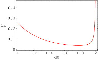
which shows how unparticles modify the usual Standard Model relation. A plot of $\lambda$ as a function of $d_{U}$ is shown in Fig. 1 for the case $m=0$, $\mu_{U}^{2}=\mu_{v}^{2}$ and $\zeta=1$. The scaling of $\lambda$ with $\mu_{U}$ and $\zeta$ can be read off from Eq. (2.21).

Having found a way of stabilizing the unparticle (and Higgs) VEVs keeping $\langle{\cal O}_{U}\rangle$ finite we can move on to the study of the combined Higgs-unparticle propagator. Perhaps the simplest way to obtain this propagator is to start with the deconstructed theory. The neutral component of the Higgs, $h^{0}$, mixes with the $\varphi_{n}$ fields in an infinite scalar mass matrix, but the secular equation can easily be obtained. Taking its continuum limit one obtains the corresponding propagator for the coupled Higgs-unparticle system (that re-sums unparticle corrections):

$\displaystyle iP(p^{2})^{-1}=p^{2}-m_{h0}^{2}+v^{2}(\mu_{U}^{2})^{2-d_{U}}\int_{0}^{\infty}\frac{(M^{2})^{d_{U}-2}}{M_{U}^{2}(M^{2})-p^{2}}r(M^{2})dM^{2}\ ,$

(3.1)

where $M_{U}^{2}(M^{2})$ is the mass distribution of unparticles after conformal symmetry breaking:

$\displaystyle M_{U}^{2}(M^{2})=M^{2}+\zeta v^{2}\ ,\;\;\;\;\;{\rm and}\;\;\;\;\;r(M^{2})=\left(\frac{M^{2}}{M^{2}+\zeta v^{2}}\right)^{2}\ .$

(3.2)

In order to understand the interplay between the Higgs and the unparticle sector after electroweak symmetry breaking it is instructive to examine the spectral representation of this propagator, which can be obtained easily.

There are two qualitatively different cases, depending on whether the Higgs mass squared $m_{h}^{2}$ is larger or smaller than $m_{gap}^{2}\equiv\zeta v^{2}$. Here $m_{h}^{2}$ is the Higgs mass corrected by the interactions to unparticles and implicitly given by the pole equation

$\displaystyle m_{h}^{2}=m_{h0}^{2}-v^{2}(\mu^{2}_{U})^{2-d_{U}}\int_{0}^{\infty}\frac{(M^{2})^{d_{U}-2}}{M_{U}^{2}(M^{2})-m_{h}^{2}}\ r(M^{2})dM^{2}\ .$

(3.3)

1. Let us first consider the case $m_{h}^{2}<\zeta v^{2}$. The analytical equation for $m_{h}^{2}$ can be explicitly written as

	$\displaystyle m_{h}^{2}$	$\displaystyle=$	$\displaystyle m_{h_{0}}^{2}-\frac{v^{2}(\mu^{2}_{U})^{2-d_{U}}}{m_{h}^{4}}\Gamma(d_{U}-1)\Gamma(2-d_{U})\times$		(3.4)
			$\displaystyle\times\left[(\zeta v^{2}-m_{h}^{2})^{d_{U}}+d_{U}m_{h}^{2}(\zeta v^{2})^{d_{U}-1}-(\zeta v^{2})^{d_{U}}\right]\ .$

Notice that the last term in (3.4) goes to zero in the (particle) limit $d_{U}\to 1$ and therefore in this limit the pole mass is the standard one, $m_{h}^{2}=m_{h_{0}}^{2}$.

The spectral function is explicitly given by

$\displaystyle\rho(s)=\frac{1}{K^{2}(m_{h}^{2})}\delta(s-m_{h}^{2})+\theta(s-\zeta v^{2})\frac{Q^{2}_{U}(s)}{\mathcal{D}^{2}(s)+\pi^{2}Q_{U}^{4}(s)}\ ,$

(3.5)

with

$\displaystyle Q^{2}_{U}(s)\equiv v^{2}(\mu_{U}^{2})^{2-d_{U}}\frac{(s-\zeta v^{2})^{d_{U}}}{s^{2}}\ ,$

(3.6)

and

$\displaystyle\mathcal{D}(s)\equiv{\mathrm{P}.V.}\left[iP(s)^{-1}\right]=s-m_{h0}^{2}+v^{2}(\mu_{U}^{2})^{2-d_{U}}\mathchoice{{\vbox{\hbox{$\textstyle-$}}\kern-4.86108pt}}{{\vbox{\hbox{$\scriptstyle-$}}\kern-3.43057pt}}{{\vbox{\hbox{$\scriptscriptstyle-$}}\kern-2.908pt}}{{\vbox{\hbox{$\scriptscriptstyle-$}}\kern-2.76045pt}}\!\int_{0}^{\infty}\frac{(M^{2})^{d_{U}-2}}{M_{U}^{2}(M^{2})-s}r(M^{2})dM^{2}\ ,$

(3.7)

where the slash in the integral denotes that its principal value should be taken. An explicit expression for $\mathcal{D}(s)$ can also be obtained analytically from (3.4). Finally,

$\displaystyle K^{2}(m_{h}^{2})\equiv\left.\frac{d}{ds}\mathcal{D}(s)\right|_{s=m_{h}^{2}}\ ,$

(3.8)

which in this case reads

$\displaystyle K^{2}(m_{h}^{2})=1+v^{2}(\mu_{U}^{2})^{2-d_{U}}\int_{0}^{\infty}\frac{(M^{2})^{d_{U}-2}}{\left[M_{U}^{2}(M^{2})-m_{h}^{2}\right]^{2}}r(M^{2})dM^{2}\ .$

(3.9)

We first notice from Eq. (3.4) that the Higgs mass at tree level is no longer simply given by $m_{h0}^{2}$ but it is shifted by a negative amount by the effect of the coupling to unparticles ²² 2 It is easy to prove that the function in the square brackets in (3.4) is positive definite for $m_{h}^{2}<m_{gap}^{2}$.. In Fig. 2 we plot the pole mass $m_{h}$ as a function of $d_{U}$ for $\mu_{U}^{2}=\mu_{v}^{2}$, $\zeta=1$ and compare it with $m_{h_{0}}$. In this case we observe that $m_{h}^{2}<m_{gap}^{2}$ for all values of $d_{U}$.

On the other hand, the coupling of the unparticle sector to the Higgs sector, that breaks the conformal symmetry, results in a modification of the “unparticle part” of the spectral function [the second term in (3.5)]. It still has no poles but now there is a mass gap, $m_{gap}$. The shape of the spectral function (3.5) is shown in Fig. 3, where we have chosen $\mu_{U}^{2}=\mu_{v}^{2}$, $\zeta=1$ and $d_{U}=1.2$, and the Higgs masses obtained from Fig. 2 are $m_{h}=115$ GeV and $m_{h_{0}}=130$ GeV. All dimensional quantities are made dimensionless by scaling them with $\zeta v^{2}$. This result for the spectral function has some similarities with that introduced in Refs. [4, 7] although it has been obtained through a different approach and differs from theirs.

Due to this mixing with the unparticles, the Higgs properties will also be affected in a way similar to the usual singlet mixing [8]. It is straightforward to obtain that the Higgs-composition of the isolated resonance at $m_{h}$, call it $R_{h}$, is simply

$\displaystyle R_{h}=\frac{1}{K(m_{h})}\ ,$

(3.10)

where $R_{h}=1$ would correspond to a pure SM Higgs with no unparticle admixture. Conversely, the unparticle continuum gets the Higgs-composition that the Higgs has lost, distributed through the $M^{2}$-dependent function

$\displaystyle R_{U}(M^{2})=-\theta(M^{2}-m_{gap}^{2})\frac{Q_{U}(M^{2})}{(M^{2}-m_{h}^{2})K(m_{h}^{2})}\ .$

(3.11)

Note that, unlike $R_{h}$, the quantity $R_{U}(M^{2})$ is a Higgs-component density and therefore has mass dimension -1. One can check that the following sum rule

$\displaystyle R_{h}^{2}+\int_{0}^{\infty}R_{U}^{2}(M^{2})\ dM^{2}=1\ ,$

(3.12)

holds. The quantities $R_{h}$ and $R_{U}(M^{2})$ play a major role in the phenomenology of Higgs and unparticles after electroweak symmetry breaking.

2. If $m_{h}^{2}>m^{2}_{gap}$, the delta function for the Higgs pole merges with the unparticle continuum. Before showing this explicitly, we first notice that the integrand in (3.3) crosses a pole and the principal value of the integral should be taken. This feature is exhibited in Fig. 4 where we plot the pole mass $m_{h}$

as a function of $d_{U}$, for $\mu_{U}^{2}=\mu_{v}^{2}$ and $\zeta=0.2$, and compare it with $m_{gap}$. We see that in the region $d_{U}\lower 3.0pt\hbox{$\,\mathrel{\mathop{\kern 0.0pt\sim}\limits^{<}}\,$}1.4$ ($d_{U}\lower 3.0pt\hbox{$\,\mathrel{\mathop{\kern 0.0pt\sim}\limits^{>}}\,$}1.4$) $m_{h}^{2}\lower 3.0pt\hbox{$\,\mathrel{\mathop{\kern 0.0pt\sim}\limits^{>}}\,$}m^{2}_{gap}$ ($m_{h}^{2}\lower 3.0pt\hbox{$\,\mathrel{\mathop{\kern 0.0pt\sim}\limits^{<}}\,$}m^{2}_{gap}$). At the value $d_{U}\simeq 1.4$ there is a kink in the integral (3.3) because the principal value has been taken. The analytical equation for $m_{h}^{2}$ now reads:

	$\displaystyle m_{h}^{2}$	$\displaystyle=$	$\displaystyle m_{h_{0}}^{2}-\frac{v^{2}(\mu^{2}_{U})^{2-d_{U}}}{m_{h}^{4}}\Gamma(d_{U}-1)\Gamma(2-d_{U})\times$		(3.13)
			$\displaystyle\times\left[(m_{h}^{2}-\zeta v^{2})^{d_{U}}\cos(\pi d_{U})+d_{U}m_{h}^{2}(\zeta v^{2})^{d_{U}-1}-(\zeta v^{2})^{d_{U}}\right]\ .$

One can also show that it is possible to have a positive shift in the Higgs mass, getting $m_{h}>m_{h0}$, for sufficiently large $m_{h}/m_{gap}$ and small enough $d_{U}$. The sign of the Higgs mass shift is shown in Fig. 5 where the positive sign corresponds to the region connected with the lower right corner.

The spectral function in this case simply reads

$\displaystyle\rho(s)=\theta(s-\zeta v^{2})\frac{Q^{2}_{U}(s)}{\mathcal{D}^{2}(s)+\pi^{2}Q_{U}^{4}(s)}\ ,$

(3.14)

with $Q^{2}_{U}(s)$ as given in (3.6). Near the Higgs pole one can approximate

$\displaystyle\mathcal{D}(s)\simeq(s-m_{h}^{2})K^{2}(m_{h}^{2})\ ,$

(3.15)

where $K^{2}(m_{h}^{2})$ is defined in Eq. (3.8). In this case one should be careful about using the principal value definition of $\mathcal{D}(s)$ to calculate properly its derivative at $m_{h}^{2}$. In fact an analytical expression for $K^{2}(m^{2}_{h})$ in this case can be simply obtained by taking the derivative of (3.13).

The shape of this spectral function is shown in Fig. 6 where we have chosen $\mu^{2}_{U}=\mu_{v}^{2}$, $\zeta=0.2$ and $d_{U}=1.2$, and the Higgs masses obtained from Fig. 4 are $m_{h}=240$ GeV and $m_{h_{0}}=245$ GeV. The peak in Fig. 6 is due to the merging of the Higgs with unparticles.

Inserting (3.15) in the spectral function (3.14) we see that the Higgs resonance has a Breit-Wigner shape of width

$\displaystyle\Gamma_{h}=\theta(m_{h}^{2}-m_{gap}^{2})\frac{\pi Q^{2}_{U}(m_{h}^{2})}{m_{h}K^{2}(m_{h}^{2})}\ .$

(3.16)

This width $\Gamma_{h}$ can be extremely wide ($\sim$ 100 GeV) depending on the parameter choices and it is plotted as a function of $d_{U}$ in Fig. 7. We can see from Fig. 7 that (as expected) it is different from zero only in the region where $m_{h}>m_{gap}$. Needless to say this kind of effect can dramatically modify the expectations for Higgs searches.

In this paper we have investigated the possibility of coupling the Higgs boson to a conformal sector of unparticles, of the type recently proposed by Georgi. A first consequence of that coupling is that electroweak symmetry breaking generates a tadpole for the unparticles. That tadpole would destabilize the theory in the absence of new interaction terms that keep the unparticle VEV finite. We have introduced for that purpose a new interaction between the Higgs and the unparticle sector using a deconstructed version of the latter.

Having stabilized the unparticle VEV we have a consistent framework in which to study the mutual influence between the Higgs and the unparticle sectors. We find changes in the properties of the Higgs (like its mass and its width) already at tree level, making the Higgs and the unparticles a mixed sector. Studying the propagator and the spectral function of this sector we find that there is a single pole, corresponding to the Higgs, with the pole mass no longer given just by the SM value, $2\lambda v^{2}$. We also find a mass gap in the formerly continuous spectral function for the unparticles, clearly indicating that the conformal symmetry has been broken. This was expected from previous work in the literature but we are able to discuss this breaking explicitly.

When the Higgs mass is greater than the unparticle mass gap, the Higgs can decay into unparticles and acquires a width which can be, in principle, very large. This can have dramatic consequences for Higgs searches at the LHC since it will mean that the Higgs will decay invisibly unless these unparticles are also coupled to the SM sector and have a sufficiently short decay length. As a last comment we can say that this is another example of how the Higgs can be the window to new sectors which would be completely hidden to us otherwise.

References

- [1] H. Georgi, Phys. Rev. Lett. 98 (2007) 221601 [hep-ph/0703260]; [hep-ph/0704.2457].
- [2] K. Cheung, W. Y. Keung and T. C. Yuan, arXiv:0704.2588 [hep-ph]
- [3] M. Luo and G. Zhu, arXiv:0704.3532 [hep-ph]; C. H. Chen and C. Q. Geng, arXiv:0705.0689 [hep-ph]; G. J. Ding and M. L. Yan, arXiv:0705.0794 [hep-ph]; Y. Liao, arXiv:0705.0837 [hep-ph]; T. M. Aliev, A. S. Cornell and N. Gaur, arXiv:0705.1326 [hep-ph]; X. Q. Li and Z. T. Wei, arXiv:0705.1821 [hep-ph]; M. Duraisamy, arXiv:0705.2622 [hep-ph]; C. D. Lu, W. Wang and Y. M. Wang, arXiv:0705.2909 [hep-ph]; N. Greiner, arXiv:0705.3518 [hep-ph]; H. Davoudiasl, arXiv:0705.3636 [hep-ph]; D. Choudhury, D. K. Ghosh and Mamta, arXiv:0705.3637 [hep-ph]; S. L. Chen and X. G. He, arXiv:0705.3946 [hep-ph]; T. M. Aliev, A. S. Cornell and N. Gaur, arXiv:0705.4542 [hep-ph]; P. Mathews and V. Ravindran, arXiv:0705.4599 [hep-ph]; S. Zhou, arXiv:0706.0302 [hep-ph]; G. J. Ding and M. L. Yan, arXiv:0706.0325 [hep-ph]; C. H. Chen and C. Q. Geng, arXiv:0706.0850 [hep-ph]; Y. Liao and J. Y. Liu, arXiv:0706.1284 [hep-ph]; M. Bander, J. L. Feng, A. Rajaraman and Y. Shirman, arXiv:0706.2677 [hep-ph]; T. G. Rizzo, arXiv:0706.3025 [hep-ph]; K. Cheung, W. Y. Keung and T. C. Yuan, arXiv:0706.3155 [hep-ph]; H. Goldberg and P. Nath, arXiv:0706.3898 [hep-ph]; S. L. Chen, X. G. He and H. C. Tsai, arXiv:0707.0187 [hep-ph]; R. Zwicky, arXiv:0707.0677 [hep-ph]; T. Kikuchi and N. Okada, arXiv:0707.0893 [hep-ph]; R. Mohanta and A. K. Giri, arXiv:0707.1234 [hep-ph]; C. S. Huang and X. H. Wu, arXiv:0707.1268 [hep-ph]; A. Lenz, arXiv:0707.1535 [hep-ph]; D. Choudhury and D. K. Ghosh, arXiv:0707.2074 [hep-ph]; H. Zhang, C. S. Li and Z. Li, arXiv:0707.2132 [hep-ph]; X. Q. Li, Y. Liu and Z. T. Wei, arXiv:0707.2285 [hep-ph]; Y. Nakayama, arXiv:0707.2451 [hep-ph]; N. G. Deshpande, X. G. He and J. Jiang, arXiv:0707.2959 [hep-ph]; T. A. Ryttov and F. Sannino, arXiv:0707.3166 [hep-th]; R. Mohanta and A. K. Giri, arXiv:0707.3308 [hep-ph].
- [4] P. J. Fox, A. Rajaraman and Y. Shirman, arXiv:0705.3092 [hep-ph].
- [5] J. R. Espinosa and M. Quirós, [hep-ph/0701145].
- [6] M. A. Stephanov, arXiv:0705.3049 [hep-ph]; N. V. Krasnikov, arXiv:0707.1419 [hep-ph].
- [7] J. Terning, G. Cacciapaglia and G. Marandella, work in progress presented at the Eötvös-Cornell 2007 Summer Workshop on Particle Physics, June 2007, Budapest.
- [8] J. R. Espinosa and J. F. Gunion, Phys. Rev. Lett. 82 (1999) 1084 [hep-ph/9807275]; J. J. van der Bij and S. Dilcher, arXiv:0707.1817 [hep-ph].