Charmonium excited state spectrum in lattice QCDPreprint: JLAB-THY-07-689
Abstract
Working with a large basis of covariant derivative-based meson interpolating fields we demonstrate the feasibility of reliably extracting multiple excited states using a variational method. The study is performed on quenched anisotropic lattices with clover quarks at the charm mass. We demonstrate how a knowledge of the continuum limit of a lattice interpolating field can give additional spin-assignment information, even at a single lattice spacing, via the overlap factors of interpolating field and state. Excited state masses are systematically high with respect to quark potential model predictions and, where they exist, experimental states. We conclude that this is most likely a result of the quenched approximation.
pacs
12.38.Gc, 12.39.Pn, 12.39.Jh, 12.40.Yx, 14.40.Gx, 11.15.HaI Introduction
In this paper we discuss an application of the variational method for extraction of spectroscopic information from lattice QCD two-point functions. We focus on the use of a large set of interpolating fields allowing access to all with sufficient redundancy to consider several excited states in each channel. As well as the usual extraction of mass information, we are also interested in the overlaps of interpolating fields on to states in the spectrum. This information is required if one wishes to extract matrix elements between hadron states from three-point or higher correlators, an example being the radiative transitions considered in Dudek et al. 2006. We find in this paper that these overlaps are also useful in aiding the spin-identification of states provided one has established the continuum behavior of the interpolating fields.
Our application of the variational method utilizes the orthogonality of states to extract excited state information. This is particularly powerful when a number of excited states are close to being degenerate - conventional multi-exponential fitting methods are not good at resolving such states. We are able to collect high statistics by the use of a small spatial volume and by confining our study to a large pseudoscalar mass , corresponding to charmonium. This volume is known to be sufficient to house the ground state for most , as illustrated for the “charge” radii extracted in Dudek et al. 2006, but we might expect it to be insufficient for radially excited states and those of high spin. We will study the volume dependence of a number of correlators and find, somewhat surprisingly, that there seems to be no meaningful difference between a box and a box.
A resurgence of interest in charmonium physics is underway, spurred by new results from BaBar, Belle and CLEO. This is reflected in increased theoretical effort, in particular there have been recent efforts to apply lattice QCD techniques to computation of quantities previously the reserve of potential models and sum-rules, such as radiative transitionsDudek et al. 2006 and two-photon decaysDudek and Edwards 2006. In this paper we extract information about the excited state and high spin spectrum, which is both interesting in its own right, and vital for concurrent attempts to extract excited state radiative transitions.
We begin in section II with a discussion of the lattice action and other computational details before in section III outlining our choice of a broad set of interpolating fields constructed to be irreducible representations of the lattice symmetry group at zero momentum and to have simple, known continuum properties. The variational method used to describe the data is explained in section IV with focus on ensuring that the solution accurately describes the input data. Spectrum results are then shown in section V, with some discussion of how continuum spin assignments can be aided by considering overlap factors. In three appendices we display properties of our interpolating fields and show an application of the variational method to toy data.
II Computational Details
The computations were performed in the quenched approximation to QCD, using the Chroma software system Edwards and Joo 2005. We employed 1000 configurations on a lattice generated using an anisotropic Wilson gauge action Klassen 1998
| (1) |
defined in terms of simple plaquettes . Here, is the bare coupling, the time component is labeled by , the spatial indices run from to , and is the bare anisotropy. We tune to the desired renormalized anisotropy where and are the spatial and temporal lattice spacings, respectively and find . The temporal lattice spacing obtained from the static quark-antiquark potential is . This gauge action is expected to have discretization errors. A smaller set of 807 configurations on a lattice were used to study finite volume effects.
Anisotropic lattices as applied to charmonium exploit the fact that while the quark mass scale demands a cut-off above , the internal three-momentum scale is typically much lower, . On our lattice, we can have both and reasonably small and a spatial length without requiring very many spatial lattice sites. Most of the work presented uses one volume, while a limited comparison is made with a large volume ; previous charmonium spectrum studies indicate that there are no significant finite volume effects for lattices of this size or largerChoe et al. 2003; Drummond et al. 2000.
The quark propagators were computed using an anisotropic version of the tadpole-improved Clover action Sheikholeslami and Wohlert 1985; Klassen 1999; Chen 2001. The Clover action we used has the “mass” form with spatial fermion tuning. Defining a lattice spacing where and , we can express this fermion action in terms of dimensionless variables , and as
| (2) |
The factor is the bare value of the fermion anisotropy. For the field strength tensor , we adopt the standard clover leaf definition. Here, the “Wilson” operator has the projector property
| (3) |
where
| (4) | |||||
| (5) |
The projector property ensures that no doubler states are present in the determined mass spectrum. We have tuned so as to yield the desired quark mass and such that the speed of light obtained from the meson dispersion relations be one, as discussed later.
We have used the tree-level conditions on and as described in Ref. Chen 2001. In particular, we will choose
| (6) |
where the ratio is set to the desired renormalized gauge anisotropy. The tadpole factors and come from the fourth-root of the spatial and temporal plaquettes, respectively, and take the values and .
The charm mass is determined by tuning the bare quark mass non-perturbatively such that the spin average of the lowest -wave mesons coincides with its experimental value, i.e. , such that . We tune non-perturbatively to satisfy the lattice dispersion relation
| (7) |
Keeping all other parameters fixed, we tune to satisfy the above relation to within and find .
We have used Dirichlet boundary conditions in the temporal direction placing the source five time-slices from the wall. All subsequent time-slice plots are with respect to this source position.
For comparison purposes, we have also used an anisotropic version of the domain-wall fermion (DWF) action Shamir 1993; Dudek et al. 2006 with a domain-wall height , a fifth dimensional extent , and a quark mass . The kernel of the domain action is the same as in Eq. 2 except without the clover terms, i.e., and set to . As in the clover case, the domain-wall quark mass and fermion anisotropy are chosen to yield the desired S-wave mass and such that the speed of light obtained from the meson dispersion relations is one.
We have computed smeared-local correlators on a subset of the same quenched lattices using both tadpole Clover and domain wall fermion quark actions. The effective masses are shown in figure 1 where we see that apart from the domain wall fermion oscillations at small times there is essentially perfect agreement between the two actions. Since the domain wall action should be improved automatically we infer that, at least for the ground state spectrum, the tadpole Clover is also improved to a good approximation.

In this study we used quenched lattices. In the spectrum of heavy quark states, where unitarity violation due to the absence of closed charm quark loops can be neglected, there are likely to be two main effects of this approximation. Firstly there are no virtual mesons in this theory and hence no thresholds for OZI-allowed decay and secondly there is the known issue of the incorrect running of the coupling and an associated ambiguity in the setting of the lattice scale. In all cases we compute only the connected contributions to correlators - the effects of disconnected contributions in charmonium are believed to be smallMcNeile and Michael 2004; de Forcrand et al. 2004.
III Interpolating Fields
It is common in meson spectroscopy calculations to focus on the simplest meson interpolating fields, namely the local fermion bilinears, . By appropriately smearing the operator over space, a large overlap on to the ground state of a given quantum number can be obtained. These operators are, however, limited in the with which they have overlap. In addition, with only these operators, while one might try various different smearings Burch et al. 2006, it is not possible to explore higher spin states. For these reasons we opt to extend the operator basis by including non-local operators, in particular ones constructed from a number of covariant derivatives acting on the quark fields. On a discretised lattice covariant derivatives become finite displacements of quark fields connected by links.
In the continuum one can construct operators which transform in a particular way under the rotation group, giving overlap only on to certain spins. On a discretized lattice the full rotation group is broken down to a smaller group of cubic rotations with a limited number of irreducible representations (irreps). The operators used in this paper are constructed to be both irreps of the lattice rotation group (at zero momentum) and to have definite, simple forms in the continuum limit. In this way we have some information about how these operators will behave in the continuum limit - we will see that this potentially aides in the interpretation of the lattice data if we are close enough to restoring rotational symmetry.
Our operators are based upon those in Liao and Manke 2002. The principal differences are that we extend the basis to include all possible zero, one and two derivative operators11 1 although not all of these are actually used in this calculation, generalize the derivatives so that the operators have definite charge-conjugation at finite momentum and correct a projection operator to ensure orthogonality within a lattice irrep. Finally we develop the continuum overlap formalism expressed in appendix A.
III.1 Derivative-based operators
In Liao and Manke 2002 single derivative operators of the type were utilized where 1 and 2 signify the flavor. The right-facing arrow indicates that the covariant derivative acts only on . For the case of a single flavor we would like the operators to be of definite charge-conjugation - it is easy to see using an integration by parts that the above operators do not achieve this at finite momentum:
| (8) |
The first term on the right-hand side has the same charge-conjugation as the left-hand side but the second term, lacking the derivative, has the opposite . This can be fixed by replacing the derivative by the quark-antiquark symmetrised . The same integration by parts as above will now not yield a term proportional to the three-momentum.
At the two-derivative level, Ref. Liao and Manke 2002 construct two combinations, and . In the -type case we ensure definite charge-conjugation at non-zero momentum by redefining . The -type case does not actually require this extension as one can easily see by expressing the pair of derivatives as the sum of a commutator and an anticommutator:
| (9) |
Clearly the -type operator is so named because it corresponds to the chromomagnetic component of the field-strength tensor. We complete the two-derivative set by adding ( is a Clebsch-Gordan coefficient as defined in the next section) and the Laplacian .
In the continuum, Lorentz symmetry along with parity and charge-conjugation specify the form of the overlap of an operator with a state of given . In appendix A we tabulate the forms, valid for all three-momenta in Minkowski space-time, for the operators we use in this paper.
We approximate covariant derivatives using finite displacements, including the appropriate links. In the results presented below we displaced only by one site, displacing by two sites was found to give correlators that did not differ considerably. Our implementation takes the form:
| (10) |
III.2 Projection onto lattice irreducible representations
Our method will be much aided by having a basis of operators that transforms irreducibly under the cubic group . The irreducible representations of O, together with their continuum spin contents, are shown in Table 1 Johnson 1982. The operators are constructed as products of gamma matrices and derivatives as outlined above, and therefore we need to project these products to their irreducible components. For operators and transforming according to the irreps and respectively, the product transforms under an element of the cubic group as
| (11) |
where is the representation matrix for the element in the irrep of dimension . The essential tool in constructing the irreps is the projection formula
| (12) |
where is a basis of operators that is reducible under the cubic group, is the representation of the rotation on that basis, and are a set of operators transforming irreducibly under the cubic group. The indices and refer to the rows of the irreducible representation, and the final step in the procedure is to identify a set of linearly independent operators as a basis for the irreducible representation.
| 1 | ||
| 1 | ||
| 2 | ||
| 3 | ||
| 3 |
Applying the projection formula 12 to the operator product of eqn. 11, we obtain
| (13) |
Identifying a set of linearly independent operators from the set , we obtain the Clebsch-Gordon coefficients for obtaining the irreducible representation in the product of operators transforming according to the irreps and :
| (14) |
In Ref. Liao and Manke 2002, the and operators are constructed via Clebsch-Gordan coefficients of to transform as , irreps respectively. The complete decomposition of is with the missing being the laplacian and the being the operator defined in the previous section. The Clebsch-Gordan coefficients in this case are where all elements are zero except
| (15) |
Examining the zero three-momentum lattice irrep projections of the continuum overlaps in appendix A, we can see that certain operators of, say, type can have overlap with higher spins only at finite with that overlap vanishing as . The simplest example is the local fermion bilinear which, transforming as can have overlap with continuum spins at finite but can only have overlap with spin-1 in the continuum. Several of our operators do retain overlap on to higher spins as , e.g. the projection of : . The non-zero overlaps in the continuum at rest are and which are linear in the spin-2 and spin-3 Minkowski polarization vectors , . None of our operators retain overlap on to spin 4 or higher in the continuum. The full set of lattice irrep projections is displayed in appendix B.
III.3 Quark and link field smearing
Constructing covariant derivatives using finite displacements with link fields can potentially produce rather noisy correlators. Any individual link is subject to large UV fluctuations over the ensemble of gauge fields. A suitable average over links neighboring a given link can help to reduce this fluctuation and providing one does this in a gauge-invariant and rotationally symmetric way, the quantum numbers of the operator will not be changed. This subject is discussed in detail in Lichtl 2006. In figure 2 we show the reduction in correlator noise we were able to obtain by judicious choice (, ) of stout-link smearing parameters.

Quark bilinear operators that are local or almost local (e.g. single site displacements) tend to have considerable overlap with a tower of states. While this can be helpful in a study like this one attempting to consider excited states, it is also useful to be able to emphasize the lower states in the spectrum. This can be achieved by smearing the quark fields over space with a gauge-invariant cubic approximation to a rotationally symmetric gaussian with any derivatives applied subsequently,
| (16) |
As well as producing improved plateaus, optimizing the quark smearing parameters does in some cases reduce noise. We show in figure 3 two representative cases. Our final parameter selection was for the local, and operators and for the operators.


IV Variational Method
Our spectrum results follow from application of a variational method to matrices of correlators. This method takes advantage of the orthogonality of state vectors on a basis of interpolating operators. The basic numerical problem to be solved is of generalized eigenvalue type
| (17) |
In this expression is the matrix of correlators at timeslice , i.e. . We transform all our operators to Minkowski space (but retain imaginary time) and in doing so ensure that this matrix is Hermitian (more detailed discussion of this point can be found in Appendix B). The generalized eigenvectors are orthonormal on the metric , . The principal correlators are the generalized eigenvalues on a given timeslice - they can be shown to behave at large times like Michael 1985; Luscher and Wolff 1990
| (18) |
where is the mass of a state labeled by and is the mass gap to the nearest state to .
Performing a Cholesky decomposition on the Hermitian matrix , where is lower diagonal, one can cast this as a conventional eigenvalue problem
| (19) |
where the eigenvectors are . These eigenvectors form a unitary matrix that transforms our “trial” operators into the optimum linear combinations to overlap with the lightest states accessible to them. The eigenvectors should be time-independent to the extent that the correlator is saturated by states; in practice we solve the eigenvalue problem on each timeslice and obtain eigenvectors that can vary with .
Clearly from the principal correlators one can extract information about the mass spectrum. There is also useful information in the eigenvectors. The conventional spectral decomposition of a two-point correlator (at zero momentum) has the form
| (20) |
where the overlap factor, . Examining the form of the generalized eigenvalue equation with substitution of the spectral decomposition one finds that
| (21) |
The inverse of the eigenvector matrix is trivial to compute owing to the orthonormality property .
In practice we work with a finite space of operators and in this case the parameter plays an important role. The eigenvectors are forced by the solution procedure to be orthogonal on the metric - this will only be a good approximation to the true orthogonality (which in the continuum is defined with an infinite number of states and operators) if the correlator at is dominated by the lightest states. As such one should choose large enough that you believe the above statement to be true. We demonstrate this using toy data in Appendix C.
In choosing a value for a given there are two factors to take into account - the above discussion suggests we should push out to larger values, where the contributions of higher excited states have decayed exponentially; however, as we do so we get into a region where the correlator data are typically noisier. As we can see from equation 19, the noise on will enter into the solution of the eigenvalue problem at all timeslices and as such we do not want to make too large. We need a criterion to decide upon an optimum value of - our choice was to define a chi-squared-like quantity gauging how well the generalized eigenvalue solution (with time-independent values) describes the correlators. At a given we solve the eigenvalue problem to yields masses (from fits to the principal correlators - details of the fitting follow later) and ’s. With these in hand we can reconstruct any correlator matrix element using equation 20. A suitable chi-squared-like quantity can be defined as
| (22) |
where and where is the data correlation matrix for the correlator computed with jackknife statistics.
The optimum value of is chosen to be that which minimizes the chi-squared-like quantity. In fact, since we solve the eigenvalue problem on each timeslice we actually get ; we choose to take the values (for a given ) from a fixed timeslice such that the chi-squared-like quantity is minimized at this . Since the are reasonably flat the chi-squared variation with is fairly mild. Insisting that the ’s are time independent for is a reflection of the fact that the only time-dependence in the spectral representation 20 is in the exponentials.
There are some subtleties that arise because we are numerically solving the generalized eigenvalue problem multiple times. One is that the phase of the eigenvector for a given state is not a quantity that can be determined with only two-point correlator information. From equation 20, it is clear that one could multiply all for a fixed by the same phase and equation 20 would be unchanged. We solve the eigenvalue problem once for each single elimination jackknife sample of our ensemble. In general the eigenproblem solver we used does not always obtain the same phase for each jackknife sample, the net effect of which is to make the configuration averages of the ’s appear to be much noisier than they really are. Our fix for this is to apply a phase convention that the largest element of the eigenvector for a given state should be positive and real.
Another subtlety can arise in the case that two (or more) states are degenerate within the level of the configuration fluctuations. In that case the solver may mis-assign a state label on any given jackknife sample (it orders according to the size of the principal correlators). This is not a serious problem for the masses since they are, in this case, equal within the error bar anyway, but for the eigenvectors it can be troublesome. On different jackknife samples one might see the eigenvector flip between two orthogonal choices with the result that the configuration average appears to be noisy. We have examined the data in this study and found that this effect does not occur at any meaningful level on our ensemble of 1000 configurations. We do, on occasion, see a flip of the eigenvector between neighboring timeslices, as we show in an example below. It is for this reason that we do not choose to average over timeslices in the determination of from .
The principal correlators are fitted using either a single exponential or a sum of two exponentials with the constraint that . The final timeslice used in the fit is chosen by the requirement that the fractional error be below and the first is selected by maximizing a fit criterion. This fit criterion also decides between the one or two exponential hypotheses.


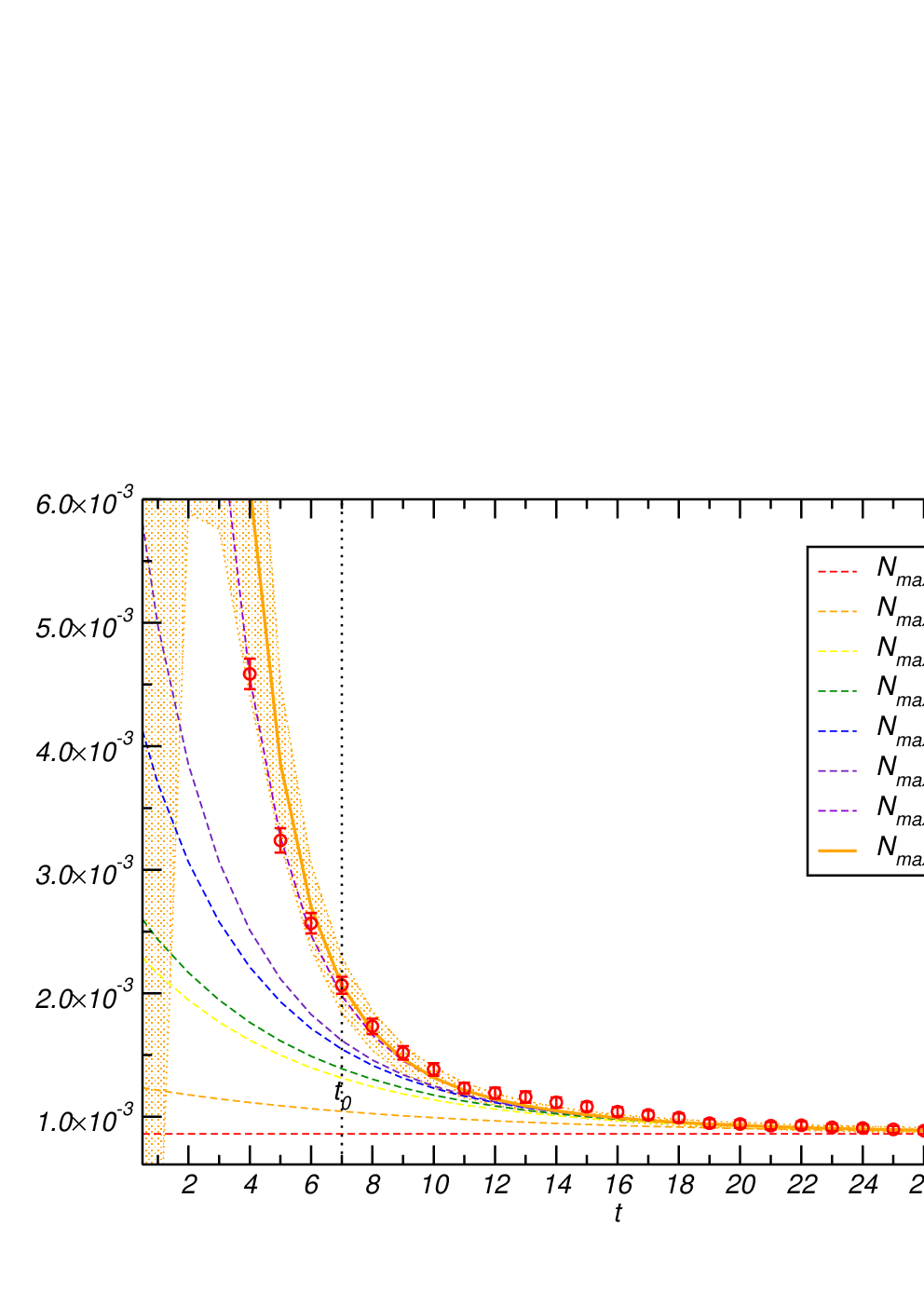

As a concrete example of our solution scheme, consider the channel in which we use the following operator basis: 22 2 Where sm and us indicate smeared and unsmeared, respectively. We solve the generalized eigenvalue problem for all between and - the -like parameter so determined is shown in figure 4, with a clear minimum being observed at . We show in figure 5 the reconstructed diagonal correlators obtained using the solution at (and ). For comparison in figure 6 we show a reconstructed diagonal correlator from the solution with . This variational method is only reliable if the eigenvectors of are orthogonal on the metric of , which only occurs if is saturated by states. In the case is not saturated by the eight states available33 3 which can also be seen in the shortfall at in the solution, indicating the need for additional states to fully describe the data at all values, and we subsequently force the eigenvectors of to be orthogonal on the “wrong” metric, a truncated metric belonging to a larger Hilbert space - this shows up at larger times as a poor description of the data. See also appendix C where this effect is investigated using toy data.
Returning to the reconstructed correlators with , we can see the power of this variational method over more conventional multi-exponential fits. Considering for example the final correlator plotted, we see that even at timeslice 7 there are at least 6 states contributing considerably to the correlator. It is unlikely that a multi-exponential fitter would converge to a solution with a sum of 6 exponentials fitting over the range 7-32. There are approximate degeneracies in the extracted spectrum and in this case the only distinguishing feature of the states are the ’s or equivalently the eigenvectors. Without enforcing orthogonality it is hard to see how one would extract meaningful information on these degenerate states.
In figure 7 we display the fits to the principal correlators of the lightest 6 states. Shown is the effective mass although we remind the reader that the correlator itself is fitted.


In figure 8 we display the extracted values for the lightest four states for the smeared operator (points with very large noise have been removed). The chi-squared-like parameter is minimized at the point which is seen to be consistent with the general trend of the data. Between timeslices 19 and 20 we see a possible example of the effect mentioned earlier that the eigenvalues for two near-degenerate states (2nd and 3rd) can flip assignment.

We note that there is not significant curvature for even though in general there can be, corresponding to higher mass states having their time-dependence placed in by the variational solver.
V Spectrum Results
In this study at zero three-momentum we opt to average correlators over diagonal directions,
| (23) | |||||
| (24) | |||||
| (25) |
It is easy to show that for the orthogonalised lattice irreps constructed these are the only non-zero entries. In general if one does not average in this way one will extract approximately degenerate states corresponding to different spin-projections ( in Appendix A) of a single state.
In the following we will discuss each combination separately.
V.1
In figure 9 we display the states extracted. The lowest band of states, at around 3500 MeV, can be identified with the near-degenerate states. In a potential model interpretation these states have an internal -wave and are split by a small spin-orbit interaction. In principle, given the continuum spin content of the lattice irreps, these states could all belong to a single state. There are a number of reasons for disfavoring such an assignment. In the channel we use only the smeared and unsmeared versions of the operator. In the continuum, the lowest dimension operator that has overlap with a spin-4 meson has three covariant derivatives - at finite lattice spacing such an operator can mix with , but must be suppressed by three powers of the lattice spacing. We expect that this is sufficient suppression relative to overlaps on to spin-0 states that we can neglect it. In fact none of the operators used in the channels have any overlap with in the continuum limit (see Appendix A), but the finite overlap is not always as suppressed as in the point-like case.
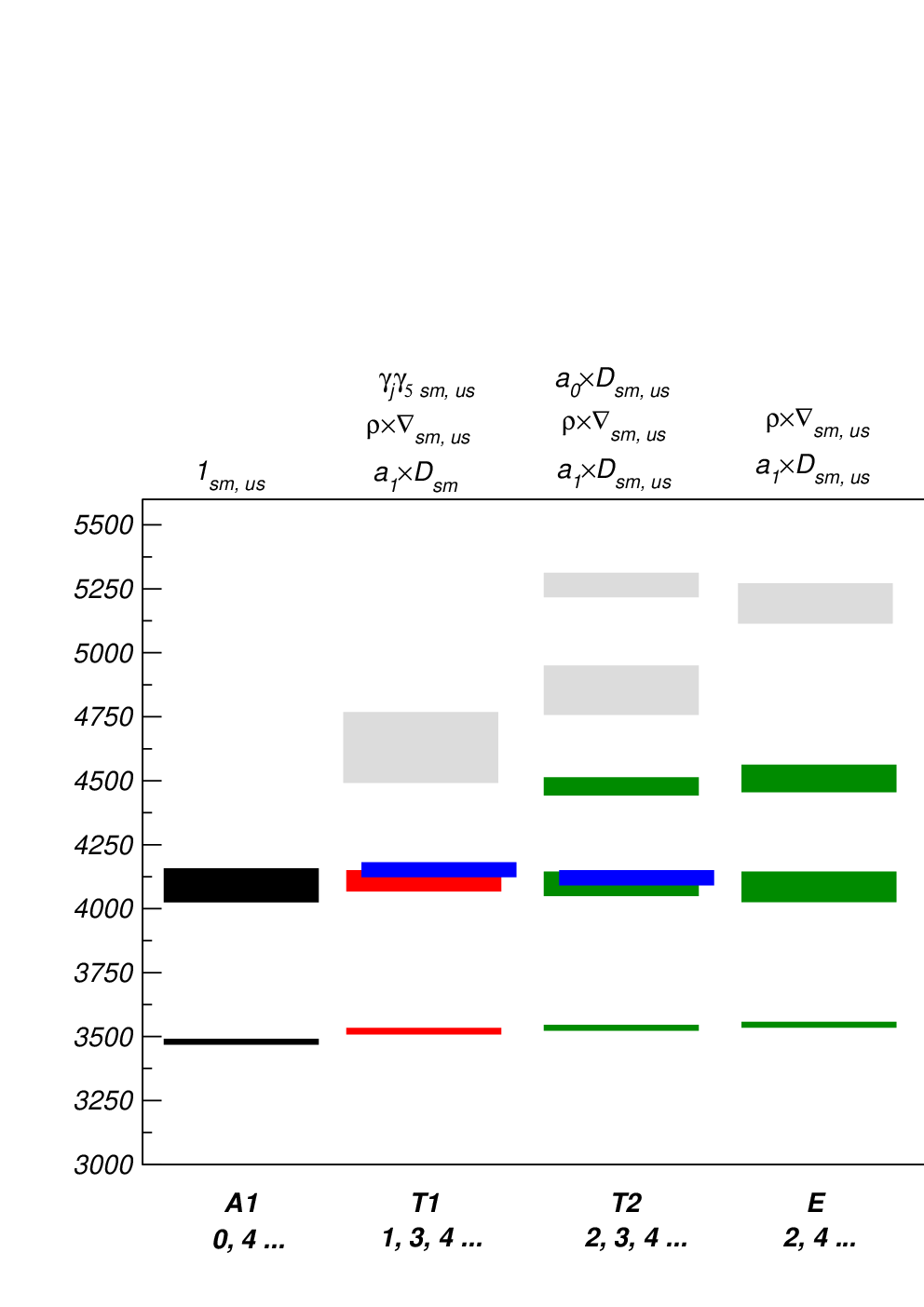

| 3477(5), 4091(61) | |
| 3523(5), 4109(36), 4152(24), 4630(133) | |
| 3534(6), 4097(42), 4121(24), 4478(30), 4854(91) | |
| 3546(6), 4085(54), 4509(48) | |
| 4170(18) |
Support beyond simply mass degeneracy for the common assignment of the lightest state in and comes from the extracted -values. Consider for example the operator - this has overlap in the continuum limit, at zero three-momentum, on to a state as follows:
| (26) |
Now, while we might think of the and irreps as being independent on a discrete lattice, their particle content is clearly related in the continuum limit, e.g. they share a common -value:
| (27) | |||||
| (28) |
We might reasonably expect that if our simulation can be considered to be “close” to the continuum limit, the -values extracted from the and channels would be related as above, up to hopefully small corrections in powers of . This is in fact what we find to a high accuracy. As a result of the correlator direction averaging described above, the relation of the extracted ’s to the defined above is . For the lightest state in we find for the smeared operator that . We take this as evidence that these states are rather close to being components of the same state.
In addition, for the unsmeared operators we find . An equivalent analysis can be applied to the operator yielding for smeared and for unsmeared, all of which appear to be compatible with a common state assignment.
The second band of states (around 4100 MeV) features a state in the irrep, which we associate with a spin-3 state in the continuum (neglecting spin-6 or higher possibilities). This state should be partnered by nearby states in the and irreps for which there are candidates being either the first or second excited states in each channel. We can use the fact that in the continuum, the and projections of the operator share a common -overlap onto the spin-3 state:
| (29) | |||||
| (30) |
With the direction averaging used we find that and . The extracted -values for the smeared operator give
| (31) |
Hence it would appear that the excited state in the channel should be partnered with the ground state in as components of a spin-3 meson. The remaining components should reside in the channel. In fact none of the operators used in that channel have overlap with in the continuum, but overlap can occur at finite through mixing with continuum operators of equal or higher dimension. For example, we have included an operator which can mix with the same-dimension operator which does have overlap with in the continuum. The degree of mixing is presumably related to a power of with at most logarithmic divergence with . At this stage we will assume that one of the states around 4100 in is a component of this spin-3 state.
The remaining states in this band then can either be components of a spin-4 meson or a nearly degenerate set. As before an argument against the option is that none of the operators used has overlap with spin-4 in the continuum - while this is likely to be a strong constraint in the , case, it is less convincing in the other channels where we include operators featuring two derivatives. Here the spin-4 overlap may only be suppressed by one power of . Explicitly we find that the overlap of the unsmeared operator onto the first excited state in is of the same magnitude as the overlap onto the ground state.
We can take the alternate route of looking for support for the hypothesis. We have already seen that there should be a definite relation between the ’s in and if the state corresponds to components of a spin-2 meson. From the fact that we have already assigned the excited state in the channel to a spin-3 meson, we’d expect that the excited states in and would have matching. In fact we find
| (32) |
While not as convincing as the ground state, we do at least see that these numbers are not inconsistent with the spin-2 hypothesis.
Giving spin assignments to higher states becomes increasingly difficult. It is no longer possible to find complete sets of components of a given spin across lattice irreps, since in certain channels we have insufficient operators to extract further states (e.g. only two operators in and hence only two states). Additionally both masses and ’s get noisier as we go higher in the spectrum. We can tentatively assign the states at around 4300 MeV in and to a on the basis of their where .
We summarize our assignments in figure 9 where they are compared to experimental charmonium states and the potential model states of Barnes et al. 2005. Discussion will follow in the next section.
V.2
Results are displayed in figure 10. The isolated lightest state in the channel can be identified as the . In this channel, there is then a large gap to the first excited state which is close to two nearly degenerate states. We anticipate the explanation of these levels as being two states and a state. In this case we believe that this is the first time that a lattice QCD calculation has observed something like the experimental pair. The extraction of such nearly degenerate states is made possible by the orthogonality properties of the variational method.


| 6106(91) | |
| 3109(2), 3722(24), 3855(12), 3843(18), 4472(79), 4442(48), 4721(42), 4957(48), 4902(85), 5126(73) | |
| 3904(36), 3904(30), 4600(42), 4933(42) | |
| 3861(24), 4817(115), 4805(42) | |
| 3861(18), 4848(54) |
The band of states around 3800 MeV has a natural explanation as a nearly degenerate set containing a state, a state and two states. The first excited state in the channel is associated with the ground state in as a meson using the -relation since .
The ground state in can be associated with the ground state in on the basis of mass degeneracy. The -relation is at the three-sigma edge of validity, . It is quite possible that this discrepancy is a discretisation effect, after all the -relations are only supposed to hold precisely in the continuum limit. To complete the we associate one of the levels in - since none of the operators we used have overlap with in the continuum we cannot apply any analysis here, although we do expect to get overlap through mixing with which has overlap with in the continuum.
A small overlap onto the unsmeared operator might be taken as signal for spin-3 nature owing to the suppression of such an overlap at , however there are also good continuum physics reasons why a spin-1 meson might have a small value of this overlap. In the non-relativistic limit this overlap measures the wavefunction at the origin of a quark-antiquark pair - while this can be considerable for an -wave state, it is zero for a state. Relativistic corrections convert this zero to a suppression relative to -wave states, see for example the experimental and .
We find that the ground state and first excited state in have comparable decay constants ( MeV and MeV) while the second and third excited states have decay constants consistent with zero ( MeV and MeV). This could be explained if they are dominantly and states. This could be investigated with simulations at smaller where we would expect one to remain finite (but small) while the other went to zero44 4 provided we included an operator with continuum overlap on to , otherwise the state would decouple altogether.
It is worth noting that these decay constants55 5 See Dudek et al. 2006 for details of scale setting of such quantities on an anisotropic lattice are larger than the experimental values. A similar result was seen for the ground state in the preliminary results of di Pierro et al. 2004. We are somewhat surprised that this value is so high considering the relative experimental agreement using domain wall fermions on the same lattices in Dudek et al. 2006. We might propose that since we are not improving our vector current operator we cannot expect the full Clover improvement, however in the improvement scheme proposed in Harada et al. 2001 there is no improvement at .
We have not been able to make spin assignments for the higher states in the spectrum for the reasons outlined in the section above. The only state we were able to extract is rather close to our temporal cutoff scale (and is compatible with the mass reported in Liu and Luo 2006) - such a state could be an exotic , but could equally well be a non-exotic . We will not comment upon it further.
We summarize our assignments in figure 10 where they are compared to experimental charmonium states and the potential model states of Barnes et al. 2005. Note that we only show those states for which we are confident of the spin assignment, the reader may assign the higher states are their own risk.
V.3
The sector has the interesting property that all states in with -even are exotic in the sense of being inaccessible to a fermion-antifermion bound state. Such states can be constructed from higher Fock states and as such are often described as being “multiquarks” (extra quark degrees of freedom) or “hybrids” (extra gluonic degrees of freedom). Adding an extra pair of charm quarks would take the state mass up to around 6 GeV, which is at the scale of our cutoff and where our quenched non-unitarity might be felt. In the physical spectrum it may be possible for light-quarks to play a non-trivial role, in this quenched study we can say nothing about this possibility. If a non-trivial gluonic field produces exotic quantum numbered states we have hope of seeing it here.


| 4521(54), 5707(79) | |
| 3525(5), 4140(42), 4000(79), 4521(48), 4497(48) | |
| 4170(73), 4733(42), 4557(139) | |
| 4593(145), 4963(248) | |
| 4218(24), 5374(91) |
Our results are displayed in figure 11. The lightest state in can be taken to be the since it has no obvious partners in other lattice irreps. We assign the set of states around 4000 MeV to a pair, support for the pairing comes from analysis of the overlaps where . Possible support for the lighter of the states being a component comes from the overlap on the operator which is consistent with zero as might be expected for an suppression. The other state has an overlap which is rather similar to the ground state and we propose that it is a .
The states around 4500 MeV are rendered somewhat non-trivial by our operator-limited knowledge of the channel. There might be other spin-3 states in this channel, but without more operators we cannot tell. If there where to be another state near 4500 MeV in we would have two plausible explanations of the states, either or . We prefer the second choice and have some support for this from the overlaps. The pairing shown in blue satisfies and we identify it with a . The higher state in have a large overlap onto and we propose it is , while the lower is consistent with zero so we tentatively assign it to , partnered by the lower state in and a missing state in . The remaining state in is then proposed to be a .
Our spin-assigned spectrum is compared with experiment and quark models in figure 11. The exotic states are somewhat lighter than the signals reported in Liao and Manke 2002; Liu and Luo 2006.
V.4
The sector again houses exotics, this time in -odd channels. We can safely assign the lowest two states in to . The lightest states in appear to make up a , and comparison appears to confirm this: . Above this spin assignment becomes treacherous. We will work under the assumption that the unexplored channel is in fact empty in our mass range - states are exotic and of high spin and might reasonably be expected to be heavy. With this we are left with two possible assignments of the states near 4300 MeV. The first would be to have two nearly degenerate states, an exotic state and a state. The second possibility is to have a single and a . Analysis of the ’s in indicates the spin-2 interpretation is at the borderline three sigma level: . The overlap of states onto is large for the ground state, the first excited state and the third excited state, but is consistent with zero for the second excited state. This might be evidence for a spin-4 nature for this state, with the overlap suppressed at .
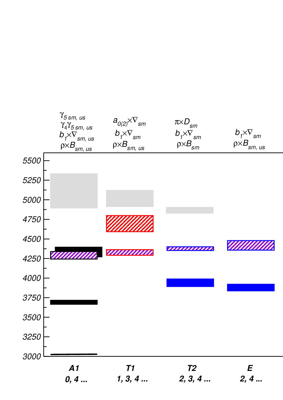


| 3024(2), 3692(24), 4291(48), 4333(61) | |
| 4327(36), 4696(103), 5017(103) | |
| 3946(48), 4376(24), 4920(48) | |
| 3879(42), 4418(61) |
We are not able with the information we have to decisively state which of the two hypothesis above is correct, and as such in figure 12 we show two possible spectrum interpretations of our data.
In figure 13 we show the effective mass of our smeared correlator along with the correlator taken from Liao and Manke 2002 computed on lattices with the same but with different anisotropy (). It is notable that the data are consistent although the fits are not.

V.5 Discussion
In our results we see thatthe masses of many excited states and states of higher spin are high with respect to the quark potential model and, where available, experimental states. We can identify three possible reasons for the systematic difference which are the three approximations in our lattice study: finite volume, non-zero and the quenched approximation66 6 and, in principle, the effect of disconnected contributions to the correlators..
The effects of a finite volume of would seem to be a likely culprit. Within potential models the wavefunction of increasingly excited and higher spin states gets support at larger and larger distances. Estimates from the potential model of Barnes, Godfrey & Swanson Swanson indicate that for example the rms radius of the first excited is already over . In order to consider this possibility we computed a limited set of correlators on a quenched lattice with all parameters identical to the simulation on . In figure 14 we show the ratio of these correlators in several typical cases where it is clear that there is no statistically significant difference, particularly in the region. To be clear we are unable to see any relevant finite-volume differences between the box and the box.


We did not study multiple lattice spacings but we can consider results in the literature for the -dependence of state masses. The studies in Okamoto et al. 2002 and Liao and Manke 2002 use rather similar actions to ours on quenched lattices and see -dependences that are relatively mild if the action is truly improved so that an extrapolation in can be performed. If a non-negligible term remains the dependence may be more significant. There typically appears to be a decrease in state masses as the continuum is approached which may explain part of our high masses.
In comparing to the quark-potential model the effect of thresholds can be neglected since their effect does not appear in this model. Hence we might expect that the principal effect of the quenched approximation would be in the incorrect running of the coupling and the associated scale-setting ambiguity. The ambiguity in scale-setting can be clearly seen in the three graphs of figure 13 in Okamoto et al. 2002. Since the wavefunctions of higher and higher excited states sample larger distances we might expect to feel even larger effects in our study. We suspect that quenching may be a major contributor to our systematically high masses.
VI Conclusions
We have investigated the use of a large basis of interpolating fields on the extraction of excited charmonium meson states in many channels. We propose an application of a variational method that systematically selects the parameter to ensure the best possible description of the data at all times greater than . We use the eigenvalues (principal correlators) to determine the mass spectrum and the eigenvectors to determine the overlaps of our interpolating fields on to the states extracted. These numbers are used herein to aid continuum spin assignment and are required quantities for study of three-point functions with the aim of extracting transition matrix elements.
The variational method has the important feature of using the orthogonality in a space of interpolating fields of different states - this is a powerful lever-arm in the extraction of near-degenerate states. In principle the method can miss states that appear in the spectrum if no linear combination of the interpolating fields used has a sufficient overlap on to the state in question; however, this is equally true of any “fitting” method and simply suggests the use of the broadest set of interpolating fields possible. With perfect statistics this analysis method should not produce any “false”, additional states in the spectrum as can happen in simple non-linear exponential fitting schemes where one adds states to minimize a chi-squared. With finite statistics and a simple ordering of eigenvalues there is the possibility that configuration-by-configuration there is state mis-assignment which can appear as several levels appearing to be degenerate within large errors. We did not observe effects like this on our sample of 1000 configurations, but with a smaller ensemble and the consequent larger fluctuations of the jackknife bins it might be expected to occur. The effect would be partnered by large fluctuations, configuration-by-configuration, of the eigenvectors, and a possible mechanism to control it would be to order the levels not simply by the size of the eigenvalue but by the similarity (via a dot-product, say) to some established basis of eigenvectors (for example comparing each single-elimination bin to the eigenvectors on the entire ensemble average).
Our interpolating fields are designed so that they have relatively simple and known overlap structures in the continuum limit, this was used to aid in the continuum spin identification of states. Supplemented with analysis at more than one lattice spacing we believe this will remove much of the possible spin ambiguity of working on a cubic lattice.
We observe in our results that our excited state masses are systematically high with respect to experiment (where it is measured) and to the potential models of Barnes et al. 2005. Our best guess is that this is a combination of not having extrapolated to the continuum limit and the effect of the quenched approximation. Both these issues can be remedied with further computation now that the efficacy of the fitting model has been demonstrated.
Arguably the most intriguing channel considered in this study is . The lowest spin contributing to this is the exotic which has been the subject of several analyses Juge et al. 2006; Mei and Luo 2003; McNeile et al. 1999; Manke et al. 1999; Liu and Luo 2006. In this study we found that we could not determine whether the lightest state in this channel (at MeV) is exotic spin-1 or non-exotic spin-4. In the potential models of Barnes et al. 2005, a non-exotic state is expected in this mass region. With the uncontrolled systematics related to quenching in this work we can have only limited bearing on phenomenology, but we lay out here the potential for misinterpretation in this channel and look forward to a relevant discussion of these matters in a future analysis with improved systematics. We note that an analysis varying the lattice spacing using the same operator set might shed light on the spin-assignment - no operators are used with have overlap on to spin-4 in the continuum, any overlap with such a state is suppressed by powers of that will reduce as . Thus a rapidly reducing would suggest a spin-4 interpretation.
Acknowledgements.
We thank Eric Swanson for his results solving a charmonium potential model in a finite box. Notice: Authored by Jefferson Science Associates, LLC under U.S. DOE Contract No. DE-AC05-06OR23177. The U.S. Government retains a non-exclusive, paid-up, irrevocable, world-wide license to publish or reproduce this manuscript for U.S. Government purposes. Computations were performed on clusters at Jefferson Laboratory as part of the USQCD collaboration.Appendix A Continuum overlaps
In this appendix we tabulate the Lorentz covariant kinematic structures corresponding to overlap of fermion bilinear interpolating fields with a limited number of Lorentz indices and states of definite . In all cases the fermion fields should be considered to be evaluated at the origin of Minkowski space time.
A.1 No Lorentz Indices
A.2 One Lorentz index
A.3 Two Lorentz indices
A.4 Three Lorentz indices
A.5 Four Lorentz indices
Here we limit ourselves to the case where the first two indices are antisymmetric and the final two have definite symmetry.
A.6 Minkowski hermitian operators
The following operators are hermitian in Minkowski space. Using these operators one is guaranteed a hermitian correlator matrix which is a requirement for the variational method.
| . |
| . |
| . |
| . |
| . |
Appendix B Lattice irrep operators at
Third column indicates the quantum numbers accessible in the continuum limit.
| op. | name | cont. | op. | name | cont. | op. | name | cont. |
|---|---|---|---|---|---|---|---|---|
| op. | name | cont. |
|---|---|---|
are the Clebsch-Gordan coefficients for . We find the non-zero values
| (33) |
Appendix C Variational analysis of toy data
In this section we consider the variational method applied to a finite spectrum of ten states when using a set of only five operators.
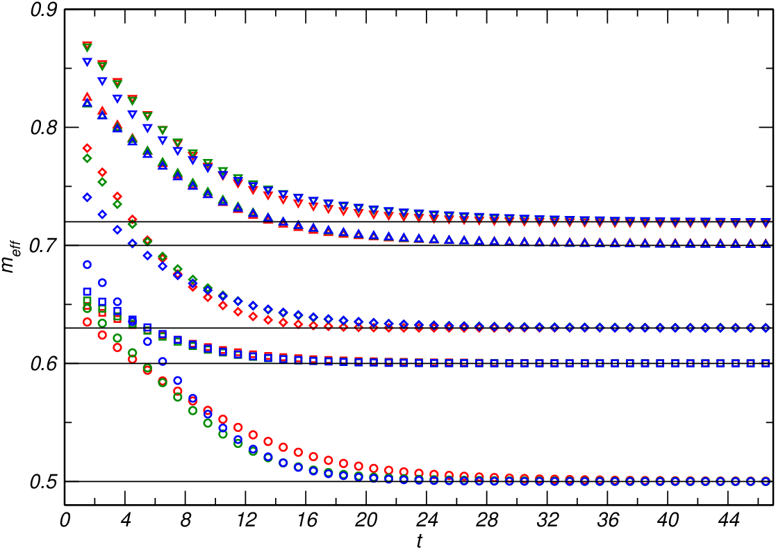
We use the mass spectrum (0.5, 0.6, 0.63, 0.7, 0.72, 0.8, 0.83, 0.9, 0.91, 1.04) proposing that there exist ideal operators which have unit-normalized overlap on to only one state, i.e. there are . We build a model analogous to a set of ’trial’ operators (linear combinations of the ideal operators) by multiplying by a random orthogonal matrix, . We construct a non-diagonal correlator matrix with elements
| (34) |
Application of the variational method to the full matrix of correlators solves the problem exactly for any value of . The situation we deal with in practice is not like this - we do not have anything like a ’complete’ basis of operators, we can model this by truncating the correlator matrix down to a submatrix.
With a selection of random orthogonal rotations () we observe a range of behaviors in the solution to the variational problem, here we show two such cases.
C.1 Case 1
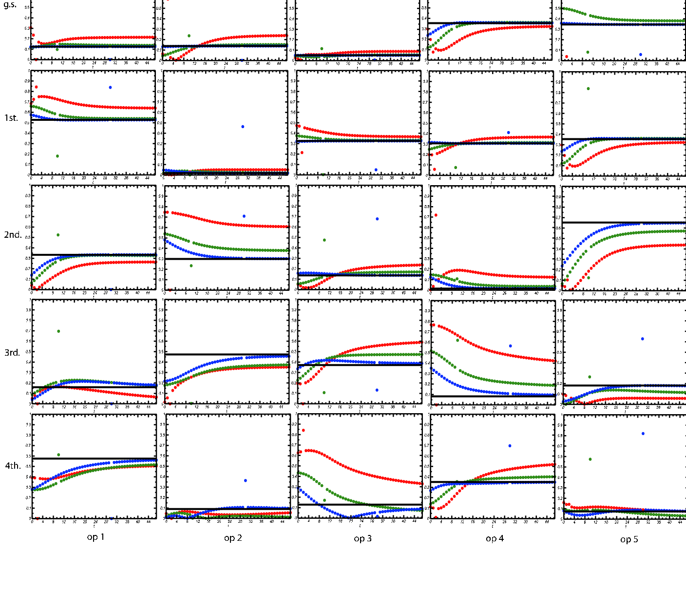
In figure 15 we show the effective masses of the principal correlators for the choices . We see that there is relatively little sensitivity in this case to the value of . On the other hand we see considerable sensitivity to in the values shown in figure 16 and only approach accurate determination of the for the largest value.
C.2 Case 2
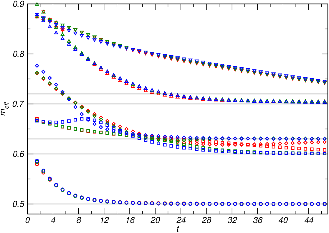
In figure 17 we show the effective masses of the principal correlators for the choices , note the qualitative differences with respect to the previous case including a flip in level ordering and the lack of a plateau in the 4th excited state. The plateaus of the first and second excited states clearly improve as is increased.
References
- Dudek et al. (2006) J. J. Dudek, R. G. Edwards, and D. G. Richards, Phys. Rev. D73, 074507 (2006), eprint hep-ph/0601137.
- Dudek and Edwards (2006) J. J. Dudek and R. G. Edwards, Phys. Rev. Lett. 97, 172001 (2006), eprint hep-ph/0607140.
- Edwards and Joo (2005) R. G. Edwards and B. Joo (SciDAC), Nucl. Phys. Proc. Suppl. 140, 832 (2005), eprint hep-lat/0409003.
- Klassen (1998) T. R. Klassen, Nucl. Phys. B533, 557 (1998), eprint hep-lat/9803010.
- Choe et al. (2003) S. Choe et al. (QCD-TARO), JHEP 08, 022 (2003), eprint hep-lat/0307004.
- Drummond et al. (2000) I. T. Drummond, N. A. Goodman, R. R. Horgan, H. P. Shanahan, and L. C. Storoni, Phys. Lett. B478, 151 (2000), eprint hep-lat/9912041.
- Sheikholeslami and Wohlert (1985) B. Sheikholeslami and R. Wohlert, Nucl. Phys. B259, 572 (1985).
- Klassen (1999) T. R. Klassen, Nucl. Phys. Proc. Suppl. 73, 918 (1999), eprint hep-lat/9809174.
- Chen (2001) P. Chen, Phys. Rev. D64, 034509 (2001), eprint hep-lat/0006019.
- Shamir (1993) Y. Shamir, Nucl. Phys. B406, 90 (1993), eprint hep-lat/9303005.
- McNeile and Michael (2004) C. McNeile and C. Michael (UKQCD), Phys. Rev. D70, 034506 (2004), eprint hep-lat/0402012.
- de Forcrand et al. (2004) P. de Forcrand et al. (QCD-TARO), JHEP 08, 004 (2004), eprint hep-lat/0404016.
- Burch et al. (2006) T. Burch et al., Phys. Rev. D74, 014504 (2006), eprint hep-lat/0604019.
- Liao and Manke (2002) X. Liao and T. Manke (2002), eprint hep-lat/0210030.
- Johnson (1982) R. C. Johnson, Phys. Lett. B114, 147 (1982).
- Lichtl (2006) A. C. Lichtl (2006), eprint hep-lat/0609019.
- Michael (1985) C. Michael, Nucl. Phys. B259, 58 (1985).
- Luscher and Wolff (1990) M. Luscher and U. Wolff, Nucl. Phys. B339, 222 (1990).
- Barnes et al. (2005) T. Barnes, S. Godfrey, and E. S. Swanson, Phys. Rev. D72, 054026 (2005), eprint hep-ph/0505002.
- di Pierro et al. (2004) M. di Pierro et al., Nucl. Phys. Proc. Suppl. 129, 340 (2004), eprint hep-lat/0310042.
- Harada et al. (2001) J. Harada, A. S. Kronfeld, H. Matsufuru, N. Nakajima, and T. Onogi, Phys. Rev. D64, 074501 (2001), eprint hep-lat/0103026.
- Liu and Luo (2006) Y. Liu and X.-Q. Luo, Phys. Rev. D73, 054510 (2006), eprint hep-lat/0511015.
- (23) E. Swanson, private Communication.
- Okamoto et al. (2002) M. Okamoto et al. (CP-PACS), Phys. Rev. D65, 094508 (2002), eprint hep-lat/0112020.
- Juge et al. (2006) K. J. Juge et al., PoS LAT2006, 193 (2006), eprint hep-lat/0610124.
- Mei and Luo (2003) Z.-H. Mei and X.-Q. Luo, Int. J. Mod. Phys. A18, 5713 (2003), eprint hep-lat/0206012.
- McNeile et al. (1999) C. McNeile et al., Nucl. Phys. Proc. Suppl. 73, 264 (1999), eprint hep-lat/9809087.
- Manke et al. (1999) T. Manke et al. (CP-PACS), Phys. Rev. Lett. 82, 4396 (1999), eprint hep-lat/9812017.