跳到论文正文
W Papers独立论文阅读器 arXiv:0707.4083 论文正文 计算阅读时间 · 0%
引用这篇论文根据当前论文元数据生成,正式投稿前建议核对。


License: Assumed arXiv.org perpetual non-exclusive license
arXiv:0707.4083v1 [cs.IT] 27 Jul 2007

Chain of Separable Binary Goppa Codes and their Minimal Distance

Sergey Bezzateev    Natalia Shekhunova Thanks: S. Bezzateev and N. Shekhunova are with the Department of Information Systems and Security , Saint Petersburg State University of Airspace Instrumentation, Saint-Petersburg, Russia, e-mail: bsv@aanet.ru, sna@delfa.net
Abstract

It is shown that subclasses of separable binary Goppa codes , Γ⁡(L,G)\Gamma(L,G) - codes, with L={α∈G​F​(22​l):G⁡(α)≠0}L=\{\alpha\in GF(2^{2l}):G(\alpha)\neq 0\} and special Goppa polynomials G⁡(x)G(x) can be presented as a chain of embedded codes. The true minimal distance has been obtained for all codes of the chain.

Index Terms: 
Goppa codes, quasi-cyclic Goppa codes, minimal distance of separable binary codes.

I Introduction

A ny qq-ary Goppa code Γ⁡(L,G)\Gamma(L,G) -code can be defined by two objects: Goppa polynomial G⁡(x)G(x) where G⁡(x)G(x) is a polynomial of a degree tt over G​F​(qm)GF(q^{m}) and location set LL where L={α∈G​F​(qm):G⁡(α)≠0}L=\{\alpha\in GF(q^{m}):G(\alpha)\neq 0\}.

Definition 1

A qq-ary vector a=(a1​…​an)a=(a_{1}...a_{n}) of a length nn where nn is a cardinality of the set L=(α1,…,αn),αi∈G​F​(qm)L=(\alpha_{1},...,\alpha_{n}),\alpha_{i}\in GF(q^{m}) is a codeword of the Γ⁡(L,G)\Gamma(L,G) Goppa code if and only if the following equation is satisfied:

∑i=1nai​1x−αi≡0​m​o​d​G​(x)\sum\limits_{i=1}^{n}a_{i}\frac{1}{x-\alpha_{i}}\equiv 0\>modG(x).

The parity check matrix of the Γ⁡(L,G)\Gamma(L,G) -code can be presented in the following form:

H=[1G⁡(α1)...1G⁡(αn)α1G⁡(α1)...αnG⁡(αn)...α1t−1G⁡(α1)...αnt−1G⁡(αn)].H=\left[\begin{array}[]{ccc}\frac{1}{G(\alpha_{1})}&...&\frac{1}{G(\alpha_{n})}\\ \frac{\alpha_{1}}{G(\alpha_{1})}&...&\frac{\alpha_{n}}{G(\alpha_{n})}\\ .&.&.\\ \frac{\alpha_{1}^{t-1}}{G(\alpha_{1})}&...&\frac{\alpha_{n}^{t-1}}{G(\alpha_{n})}\end{array}\right].

It is known that the Γ⁡(L,G)\Gamma(L,G) -code has following parameters [1]:

the length of the code is equal to the cordinality nn of the location set LL, n≤qmn\leq q^{m}

the dimension is k≥n−t​mk\geq n-tm and

the true minimal distance is d≥t+1d\geq t+1.

The Γ⁡(L,G)\Gamma(L,G)-code is a binary Goppa code if q=2q=2.

The Γ⁡(G,L)\Gamma(G,L)- code is a separable Goppa code if all roots of its Goppa polynomial GG are different.

The following estimation of the true minimal distance for binary separable (L,G)-codes is valid [1]:

d≥2​t+1d\geq 2t+1.

Binary separable Goppa codes have been studied by many authors. The binary separable codes with the location set over G​F​(2s​l)GF(2^{sl}) where s=2,3,…s=2,3,... are of the greatest interest.

M. Loeloeian and J. Conan were the first who considered the code of this class. In 1984 they presented[2] the best known (55,16,19)- Goppa code with the Goppa polynomial:

G(x)=(x−α9)(˙x−α12)(˙x−α30)(˙x−α34)(˙x−α42)(˙x−α43)(˙x−α50)(˙x−α54)G(x)=(x-\alpha^{9})\dot{(}x-\alpha^{12})\dot{(}x-\alpha^{30})\dot{(}x-\alpha^{34})\dot{(}x-\alpha^{42})\dot{(}x-\alpha^{43})\dot{(}x-\alpha^{50})\dot{(}x-\alpha^{54})

where α\alpha is a primitive element of G​F​(26).GF(2^{6}).

In 1986 we considered [3] this code as a code from a subclass of Goppa codes with the Goppa polynomial:
G⁡(x)=xt+1+Vt​xt+V​x+1G(x)=x^{t+1}+V^{t}x^{t}+Vx+1
where V∈G​F​(22​l)V\in GF(2^{2l}) , t=2lt=2^{l} , L⊂G​F​(22​l)L\subset GF(2^{2l}) and n=22​l−t−1n=2^{2l}-t-1.
We have proved [3], [4] that the dimension of these codes is
k≥n−2​l​(t−32)k\geq n-2l(t-\frac{3}{2}).

In 1987 M. Loeloeian and J. Conan [5] considered a subclass of Goppa codes with the Goppa polynomial:
G⁡(x)=xt+xG(x)=x^{t}+x
where t=2lt=2^{l} ,L⊂G​F​(22​l)L\subset GF(2^{2l}) and n=22​l−tn=2^{2l}-t.
They also gave the estimation for the dimension of these codes:
k≥n−2​l​(t−32)−1.k\geq n-2l(t-\frac{3}{2})-1.

The same estimation for the dimension of these codes was obtained by A.M.Roseiro, J.I.Hall, J.E.Adney and M.Siegel in [6] by using the kernel of an associated trace map. In this paper, the subclass of codes with polynomial G⁡(x)=xt+xG(x)=x^{t}+x was called as quadratic trace Goppa codes.

In 1995 we described [7] the subclass of Goppa codes with the polynomial G⁡(x)=xt−1+1G(x)=x^{t-1}+1 and we have proved that the minimal distance of these codes is equal to their design distance.

In 2001 P. Veron [8] investigated the structure of trace Goppa codes and proved that the true dimension for these codes is equal to the estimation obtained previously:
k≥n−2​l​(t−32)−1k\geq n-2l(t-\frac{3}{2})-1

In 2005 P. Veron [9] proved that the estimation of the code dimension for Goppa codes with G⁡(x)=xt+1+Vt​xt+V​x+1G(x)=x^{t+1}+V^{t}x^{t}+Vx+1 and G⁡(x)=xt−1+1G(x)=x^{t-1}+1 is the true dimension for the codes from this subclasses [10].

In [11] and also in [12] (G. Bommer and F. Blanchet) and in [13] (P. Veron) it was proved that all the mentioned above codes are a quasi-cyclic binary Goppa codes.

In 2007 G.Maatouk, A.Shokrollahi and M.Cheraghchi [14] tried to prove that the class of codes which was described in [7] achieved the GV bound.

In this paper, we present all codes that were mentioned above as a chain of embedded codes. We obtain the true minimal distance for these codes. The rest of the paper is organized as follows.

Section 2 describes the chain of Goppa codes subclasses.

Section 3 gives several Lemmas for the true minimal distance for subfield subcodes:
G5​(x)=C​xt+1+At​xt+A​xG_{5}(x)=Cx^{t+1}+A^{t}x^{t}+Ax,
G6​(x)=R​xt+1+Vt​xt+V​x+1G_{6}(x)=Rx^{t+1}+V^{t}x^{t}+Vx+1
where R∈G​F​(2l),V∈G​F​(22​l)R\in GF(2^{l}),V\in GF(2^{2l}) and G7​(x)=xt+1+1.G_{7}(x)=x^{t+1}+1.

In Section 4 similar Lemmas are presented for quadratic trace Goppa codes:
G2​(x)=At​xt+A​xG_{2}(x)=A^{t}x^{t}+Ax and
G3​(x)=At​xt+A​x+CG_{3}(x)=A^{t}x^{t}+Ax+C,
where A∈G​F​(22​l)A\in GF(2^{2l}) and C∈G​F​(2l)C\in GF(2^{l})).

In Section 5 we obtain the true minimal distance for codes that are not subfield or trace codes: these new codes with a Goppa polynomial
G4​(x)=At​xt+At−1​xt−1+1G_{4}(x)=A^{t}x^{t}+A^{t-1}x^{t-1}+1
have not been described before.

In Conclussion a table with parameters of codes from the code chain and table of binary quasi-cyclic codes from this chain are presented.

II Code chain

Let us show how to obtain one code from another and to create a family of embedded codes, a so-called chain of codes.

Definition 2

Let matrix H1∗H_{1}^{\ast} be a parity check matrix of the binary Goppa code with a location set L1∗={αi1,αi2,…,αin}L_{1}^{\ast}=\{\alpha_{i_{1}},\alpha_{i_{2}},...,\alpha_{i_{n}}\} of different nonzero elements from G​F​(22​l)GF(2^{2l}) such that αijt−1≠1\alpha_{i_{j}}^{t-1}\neq 1 for all j=1,..,nj=1,..,n and Goppa polynomial G1​(x)=xt−1+1,t=2lG_{1}(x)=x^{t-1}+1,t=2^{l} :

H1∗=[1αi1t−1+1...1αint−1+1αi1αi1t−1+1...αinαint−1+1...αi1t−1αi1t−1+1...αint−1αint−1+1].H_{1}^{\ast}=\left[\begin{array}[]{ccc}\frac{1}{\alpha_{{}_{i_{1}}}^{t-1}+1}&...&\frac{1}{\alpha_{i_{{}_{n}}}^{t-1}+1}\\ \frac{\alpha_{i_{1}}}{\alpha_{i_{1}}^{t-1}+1}&...&\frac{\alpha_{i_{n}}}{\alpha_{i_{{}_{n}}}^{t-1}+1}\\ .&.&.\\ \frac{\alpha_{i_{1}}^{t-1}}{\alpha_{i_{1}}^{t-1}+1}&...&\frac{\alpha_{i_{n}}^{t-1}}{\alpha_{i_{{}_{n}}}^{t-1}+1}\end{array}\right].

Lemma 1

A row [1αi1(αi1t−1+1)...1αin(αint−1+1)]\left[\begin{array}[]{ccc}\frac{1}{\alpha_{i_{1}}(\alpha_{{}_{i_{1}}}^{t-1}+1)}&...&\frac{1}{\alpha_{i_{{}_{n}}}(\alpha_{i_{n}}^{t-1}+1)}\end{array}\right] can be represented as a linear combination of corresponding rows from the matrix H1∗H_{1}^{\ast}.

Proof:

For any α∈L1∗\alpha\in L_{1}^{\ast}

α2l−1−1αt−1+1=α2l−1−1α(t−1)​(α−(t−1)+1)=1α2l−1​(α−(t−1)+1)=1α2l−1​(αt−1+1)2l=(1α​(αt−1+1)2)2l−1.\frac{\alpha^{2^{l-1}-1}}{\alpha^{t-1}+1}=\frac{\alpha^{2^{l-1}-1}}{\alpha^{(t-1)}(\alpha^{-(t-1)}+1)}=\frac{1}{\alpha^{2^{l-1}}(\alpha^{-(t-1)}+1)}=\frac{1}{\alpha^{2^{l-1}}(\alpha^{t-1}+1)^{2^{l}}}=\left(\frac{1}{\alpha(\alpha^{t-1}+1)^{2}}\right)^{2^{l-1}}.

Therefore the row [1αi1(αi1t−1+1)2...1αin(αint−1+1)2]\left[\begin{array}[]{ccc}\frac{1}{\alpha_{i_{1}}(\alpha_{{}_{i_{1}}}^{t-1}+1)^{2}}&...&\frac{1}{\par\alpha_{i_{{}_{n}}}(\alpha_{i_{{}_{n}}}^{t-1}+1)^{2}}\end{array}\right] can be obtained from the row [αi12l−1−1αi1t−1+1...αin2l−1−1αint−1+1]\left[\begin{array}[]{ccc}\frac{\alpha_{i_{1}}^{2^{l-1}-1}}{\alpha_{i_{1}}^{t-1}+1}&...&\frac{\alpha_{i_{n}}^{2^{l-1}-1}}{\alpha_{i_{{}_{n}}}^{t-1}+1}\end{array}\right] of the matrix H1∗H_{1}^{\ast} .

For any α∈L1∗\alpha\in L_{1}^{\ast}

1α​(αt−1+1)2+(α2l−1−1(αt−1+1))2=1α​(αt−1+1)2+α2l−2(αt−1+1)2=1α​(αt−1+1)2+α2l−1α​(αt−1+1)2=1α⁡(αt−1+1)\frac{1}{\alpha(\alpha^{t-1}+1)^{2}}+\left(\frac{\alpha^{2^{l-1}-1}}{(\alpha^{t-1}+1)}\right)^{2}=\frac{1}{\alpha(\alpha^{t-1}+1)^{2}}+\frac{\alpha^{2^{l}-2}}{(\alpha^{t-1}+1)^{2}}=\frac{1}{\alpha(\alpha^{t-1}+1)^{2}}+\frac{\alpha^{2^{l}-1}}{\alpha(\alpha^{t-1}+1)^{2}}=\frac{1}{\alpha(\alpha^{t-1}+1)} .

Therefore the row [1αi1(αi1t−1+1)...1αin(αint−1+1)]\left[\begin{array}[]{ccc}\frac{1}{\alpha_{i_{1}}(\alpha_{{}_{i_{1}}}^{t-1}+1)}&...&\frac{1}{\alpha_{i_{{}_{n}}}(\alpha_{i_{{}_{n}}}^{t-1}+1)}\end{array}\right] can be obtained from the row [αi12l−1−1αi1t−1+1...αin2l−1−1αint−1+1]\left[\begin{array}[]{ccc}\frac{\alpha_{i_{1}}^{2^{l-1}-1}}{\alpha_{i_{1}}^{t-1}+1}&...&\frac{\alpha_{i_{n}}^{2^{l-1}-1}}{\alpha_{i_{{}_{n}}}^{t-1}+1}\end{array}\right] of the matrix H1∗H_{1}^{\ast}. ∎

Corollary 1

By using the result of Lemma 1 we can rewrite the matrix H1∗H_{1}^{\ast} in the following form:

H1∗=[1αi1(αi1t−1+1)...1αin(αint−1+1)1αi1t−1+1...1αint−1+1αi1αi1t−1+1...αinαint−1+1...αi1t−1αi1t−1+1...αint−1αint−1+1].H_{1}^{\ast}=\left[\begin{array}[]{ccc}\frac{1}{\alpha_{{}_{i_{1}}}\left(\alpha_{{}_{i_{1}}}^{t-1}+1\right)}&...&\frac{1}{\alpha_{i_{{}_{n}}}\left(\alpha_{i_{{}_{n}}}^{t-1}+1\right)}\\ \frac{1}{\alpha_{{}_{i_{1}}}^{t-1}+1}&...&\frac{1}{\alpha_{i_{{}_{n}}}^{t-1}+1}\\ \frac{\alpha_{i_{1}}}{\alpha_{i_{1}}^{t-1}+1}&...&\frac{\alpha_{i_{n}}}{\alpha_{i_{{}_{n}}}^{t-1}+1}\\ .&.&.\\ \frac{\alpha_{i_{1}}^{t-1}}{\alpha_{i_{1}}^{t-1}+1}&...&\frac{\alpha_{i_{n}}^{t-1}}{\alpha_{i_{{}_{n}}}^{t-1}+1}\end{array}\right].

Now let us obtain the parity check matrix H1H_{1} for a code Γ⁡(L1,G1)\Gamma(L_{1},G_{1}) with G1​(x)=xt−1+1,t=2lG_{1}(x)=x^{t-1}+1,\ t=2^{l} and L1={α1,α2,…,αn1−1,0},n1=22​l−2l+1:L_{1}=\{\alpha_{1},\alpha_{2},...,\alpha_{n_{1}-1},0\},\ n_{1}=2^{2l}-2^{l}+1:

H1=[1α1t−1+1...1αn1−1t−1+11α1α1t−1+1...αn1−1αn1−1t−1+10....α1t−1α1t−1+1...αn1−1t−1αn1−1t−1+10].H_{1}=\left[\begin{array}[]{cccc}\frac{1}{\alpha_{1}^{t-1}+1}&...&\frac{1}{\alpha_{n_{1}-1}^{t-1}+1}&1\\ \frac{\alpha_{1}}{\alpha_{1}^{t-1}+1}&...&\frac{\alpha_{n_{1}-1}}{\alpha_{n_{1}-1}^{t-1}+1}&0\\ .&.&.&.\\ \frac{\alpha_{1}^{t-1}}{\alpha_{1}^{t-1}+1}&...&\frac{\alpha_{n_{1}-1}^{t-1}}{\alpha_{n_{1}-1}^{t-1}+1}&0\end{array}\right].

By using the power 2l2^{l} of the first row from H1H_{1} we obtain:

[α1t−1α1t−1+1...αn1−1t−1αn1−1t−1+11].\left[\begin{array}[]{cccc}\frac{\alpha_{1}^{t-1}}{\alpha_{1}^{t-1}+1}&...&\frac{\alpha_{n_{1}-1}^{t-1}}{\alpha_{n_{1}-1}^{t-1}+1}&1\end{array}\right].

The sum of this row and the first row from the matrix H1H_{1} gives us

[α1t−1α1t−1+1...αn1−1t−1αn1−1t−1+11]+[1α1t−1+1...1αn1−1t−1+11]=[1...10].\left[\begin{array}[]{cccc}\frac{\alpha_{1}^{t-1}}{\alpha_{1}^{t-1}+1}&...&\frac{\alpha_{n_{1}-1}^{t-1}}{\alpha_{n_{1}-1}^{t-1}+1}&1\end{array}\right]+\left[\begin{array}[]{cccc}\frac{1}{\alpha_{1}^{t-1}+1}&...&\frac{1}{\alpha_{n_{1}-1}^{t-1}+1}&1\end{array}\right]=\left[\begin{array}[]{cccc}1&...&1&0\end{array}\right].

Therefore the parity check matrix H1H_{1} can be rewritten:

H1=[1α1t−1+1...1αn1−1t−1+11α1α1t−1+1...αn1−1αn1−1t−1+10....α1t−1α1t−1+1...αn1−1t−1αn1−1t−1+101...10].H_{1}=\left[\begin{array}[]{cccc}\frac{1}{\alpha_{1}^{t-1}+1}&...&\frac{1}{\alpha_{n_{1}-1}^{t-1}+1}&1\\ \frac{\alpha_{1}}{\alpha_{1}^{t-1}+1}&...&\frac{\alpha_{n_{1}-1}}{\alpha_{n_{1}-1}^{t-1}+1}&0\\ .&.&.&.\\ \frac{\alpha_{1}^{t-1}}{\alpha_{1}^{t-1}+1}&...&\frac{\alpha_{n_{1}-1}^{t-1}}{\alpha_{n_{1}-1}^{t-1}+1}&0\\ 1&...&1&0\end{array}\right].

Let us define a parity check matrix for a subcode Γ⁡(L1∗,G1)\Gamma(L_{1}^{\ast},G_{1}) of the code Γ⁡(L1,G1)\Gamma(L_{1},G_{1}) ,
L1∗=L1\{0}={α1,α2,…,αn1−1}\qquad L_{1}^{\ast}=L_{1}\backslash\{0\}=\{\alpha_{1},\alpha_{2},...,\alpha_{n_{1}-1}\}, n1∗=n1−1.n_{1}^{\ast}=n_{1}-1.

[1α1t−1+1...1αn1−1t−1+1α1α1t−1+1...αn1−1αn1−1t−1+1...α1t−1α1t−1+1...αn1−1t−1αn1−1t−1+11...1]=[H1∗1​…​1].\left[\begin{array}[]{ccc}\frac{1}{\alpha_{1}^{t-1}+1}&...&\frac{1}{\alpha_{n_{1}-1}^{t-1}+1}\\ \frac{\alpha_{1}}{\alpha_{1}^{t-1}+1}&...&\frac{\alpha_{n_{1}-1}}{\alpha_{n_{1}-1}^{t-1}+1}\\ .&.&.\\ \frac{\alpha_{1}^{t-1}}{\alpha_{1}^{t-1}+1}&...&\frac{\alpha_{n_{1}-1}^{t-1}}{\alpha_{n_{1}-1}^{t-1}+1}\\ 1&...&1\end{array}\right]=\left[\begin{array}[]{c}H_{1}^{\ast}\\ 1...1\end{array}\right].

Lemma 2

Γ⁡(L1∗,G1)≡Γ⁡(L2,G2)\Gamma(L_{1}^{\ast},G_{1})\equiv\Gamma(L_{2},G_{2}) where G1​(x)=xt−1+1G_{1}(x)=x^{t-1}+1 and G2​(x)=At​xt+A​x,t=2l,G_{2}(x)=A^{t}x^{t}+Ax,\ t=2^{l}, AA ∈G​F​(22​l)\in GF(2^{2l}).

Proof:

Obviously, Γ⁡(L1,G2)≡Γ⁡(L2,G2∗)\Gamma(L_{1},G_{2})\equiv\Gamma(L_{2},G_{2}^{\ast}) where G2∗​(x)=xt+x=x∗G1​(x)G_{2}^{\ast}(x)=x^{t}+x=x\ast G_{1}(x) and the Goppa polynomial G2​(x)=At​xt+A​xG_{2}(x)=A^{t}x^{t}+Ax can be obtained from G2∗​(x)G_{2}^{\ast}(x) by using the A​xAx substitution for a variable xx, AA ∈G​F​(22​l)\in GF(2^{2l}).

A parity check matrix H2H_{2} for the code Γ⁡(L2,G2∗)\Gamma(L_{2},G_{2}^{\ast}) with G2∗​(x)=xt+x,t=2lG_{2}^{\ast}(x)=x^{t}+x,\ t=2^{l} and L2={α1,α2,…,αn2},n2=22​l−2lL_{2}=\{\alpha_{1},\alpha_{2},...,\alpha_{n_{2}}\},\ n_{2}=2^{2l}-2^{l} is :

H2=[1α1t+α1...1αn2t+αn2α1α1t+α1...αn2αn2t+αn2...α1t−1α1t+α1...αn2t−1αn2t+αn2].H_{2}=\left[\begin{array}[]{ccc}\frac{1}{\alpha_{1}^{t}+\alpha_{1}}&...&\frac{1}{\alpha_{n_{2}}^{t}+\alpha_{n_{2}}}\\ \frac{\alpha_{1}}{\alpha_{1}^{t}+\alpha_{1}}&...&\frac{\alpha_{n_{2}}}{\alpha_{n_{2}}^{t}+\alpha_{n_{2}}}\\ .&.&.\\ \frac{\alpha_{1}^{t-1}}{\alpha_{1}^{t}+\alpha_{1}}&...&\frac{\alpha_{n_{2}}^{t-1}}{\alpha_{n_{2}}^{t}+\alpha_{n_{2}}}\end{array}\right].

It is easy to see that this matrix can be rewritten in the following form:

H2=[1α1​(α1t−1+1)...1αn2​(αn2t−1+1)1α1t−1+1...1αn2t−1+1...α1t−2α1t−1+1...αn2t−2αn2t−1+1]H_{2}=\left[\begin{array}[]{ccc}\frac{1}{\alpha_{1}\left(\alpha_{1}^{t-1}+1\right)}&...&\frac{1}{\alpha_{n_{2}}\left(\alpha_{n_{2}}^{t-1}+1\right)}\\ \frac{1}{\alpha_{1}^{t-1}+1}&...&\frac{1}{\alpha_{n_{2}}^{t-1}+1}\\ .&.&.\\ \frac{\alpha_{1}^{t-2}}{\alpha_{1}^{t-1}+1}&...&\frac{\alpha_{n_{2}}^{t-2}}{\alpha_{n_{2}}^{t-1}+1}\end{array}\right]

From Corollary 1 the matrix H2\ H_{2} is equal to the matrix H1∗H_{1}^{\ast} , therefore Γ⁡(L1∗,G1)≡Γ⁡(L2,G2∗)≡Γ⁡(L2,G2).\Gamma(L_{1}^{\ast},G_{1})\equiv\Gamma(L_{2},G_{2}^{\ast})\equiv\Gamma(L_{2},G_{2}). ∎

(This statement has been proved by P.Veron in [13],[9] by using another approach.)

Lemma 3

Γ⁡(L2,G2)≡Γ⁡(L3,G3)\Gamma(L_{2},G_{2})\equiv\Gamma(L_{3},G_{3}) where G3​(x)=At​xt+A​x+CG_{3}(x)=A^{t}x^{t}+Ax+C, C∈G​F​(2l)C\in GF(2^{l}) and AA ∈G​F​(22​l)\in GF(2^{2l}).

Proof:

Using the x+βx+\beta substitution for a variable xx where β∈G​F​(22​l)\beta\in GF(2^{2l}) and β≠A−(t−1)\beta\neq A^{-(t-1)} we obtain:

G2​(x+β)=At​(x+β)t+A⁡(x+β)=At​xt+A​x+(At​βt+A​β)G_{2}(x+\beta)=A^{t}(x+\beta)^{t}+A(x+\beta)=A^{t}x^{t}+Ax+(A^{t}\beta^{t}+A\beta)
where (At​βt+A​β)2l=(A​β+At​βt)(A^{t}\beta^{t}+A\beta)^{2^{l}}=(A\beta+A^{t}\beta^{t}) follows from the conditions of Lemma 3. Therefore C=At​βt+A​βC=A^{t}\beta^{t}+A\beta , CC ∈G​F​(2l)\in GF(2^{l}) and G2​(x+β)=At​xt+A​x+C=G3​(x)G_{2}(x+\beta)=A^{t}x^{t}+Ax+C=G_{3}(x) . ∎

Lemma 4

All codewords of the code Γ⁡(L4,G4)\Gamma(L_{4},G_{4}) with G4​(x)=At​xt+At−1​xt−1+1G_{4}(x)=A^{t}x^{t}+A^{t-1}x^{t-1}+1 have the zero value on the position correspondig to the element 00 from L4={α1,α2,…,αn4−1,0}L_{4}=\{\alpha_{1},\alpha_{2},...,\alpha_{n_{4}-1},0\}.

Proof:

Obviously, by substituting xx to A−1​xA^{-1}x in G4​(x)G_{4}(x) we obtain the same Γ⁡(L4,G4)\Gamma(L_{4},G_{4}) code with a more simple Goppa polynomial: G4​(x)=xt+xt−1+1.G_{4}(x)=x^{t}+x^{t-1}+1.

Let us consider the parity check matrix of this code:

H4=[1α1t+α1t−1+1...1αn4−1t+αn4−1t−1+11α1α1t+α1t−1+1...αn4−1αn4−1t+αn4−1t−1+10....α1t−1α1t+α1t−1+1...α1t−1αn4−1t+αn4−1t−1+10].H_{4}=\left[\begin{array}[]{cccc}\frac{1}{\alpha_{1}^{t}+\alpha_{1}^{t-1}+1}&...&\frac{1}{\alpha_{n_{4}-1}^{t}+\alpha_{n_{4}-1}^{t-1}+1}&1\\ \frac{\alpha_{1}}{\alpha_{1}^{t}+\alpha_{1}^{t-1}+1}&...&\frac{\alpha_{n_{4}-1}}{\alpha_{n_{4}-1}^{t}+\alpha_{n_{4}-1}^{t-1}+1}&0\\ .&.&.&.\\ \frac{\alpha_{1}^{t-1}}{\alpha_{1}^{t}+\alpha_{1}^{t-1}+1}&...&\frac{\alpha_{1}^{t-1}}{\alpha_{n_{4}-1}^{t}+\alpha_{n_{4}-1}^{t-1}+1}&0\end{array}\right].

By using the t−t-th degree of the first row of this parity check matrix we can obtain the following parity check row for Γ⁡(L4,G4):\Gamma(L_{4},G_{4}):

rr=[α1t−1α1t+α1t−1+1...α1t−1αn4−1t+αn4−1t−1+11]\left[\begin{array}[]{cccc}\frac{\alpha_{1}^{t-1}}{\alpha_{1}^{t}+\alpha_{1}^{t-1}+1}&...&\frac{\alpha_{1}^{t-1}}{\alpha_{n_{4}-1}^{t}+\alpha_{n_{4}-1}^{t-1}+1}&1\end{array}\right].

For this row and for the last row of the parity check matrix H4H_{4} and parity check row rr for any codeword a=(a1​…​an4)a=(a_{1}...a_{n_{4}}) of the code Γ⁡(L4,G4)\Gamma(L_{4},G_{4}) the following expressions are valid:

∑i=1n4−1ai​αit−1αit+αit−1+1=0\sum\limits_{i=1}^{n_{4}-1}a_{i}\frac{\alpha_{i}^{t-1}}{\alpha_{i}^{t}+\alpha_{i}^{t-1}+1}=0 and ∑i=1n4−1ai​αit−1αit+αit−1+1=an4.\sum\limits_{i=1}^{n_{4}-1}a_{i}\frac{\alpha_{i}^{t-1}}{\alpha_{i}^{t}+\alpha_{i}^{t-1}+1}=a_{n_{4}}.

It is possible only in case when an4=0a_{n_{4}}=0 for all codewords of the code Γ⁡(L4,G4).\Gamma(L_{4},G_{4}). ∎

Corollary 2

The code Γ⁡(L4,G4)\Gamma(L_{4},G_{4}) is equal to the code Γ⁡(L4∗,G4)\Gamma(L_{4}^{\ast},G_{4}) with n4∗=n4−1n_{4}^{\ast}=n_{4}-1, k4∗=k4k_{4}^{\ast}=k_{4} and L4∗={α1,α2,…,αn4−1}L_{4}^{\ast}=\{\alpha_{1},\alpha_{2},...,\alpha_{n_{4}-1}\}.

The parity check matrix H4∗H_{4}^{\ast}of the code Γ⁡(L4∗,G4)\Gamma(L_{4}^{\ast},G_{4}) is:

H4∗=[1α1t+α1t−1+1...1αn4−1t+αn4−1t−1+1α1α1t+α1t−1+1...αn4−1αn4−1t+αn4−1t−1+1...α1t−1α1t+α1t−1+1...α1t−1αn4−1t+αn4−1t−1+1]H_{4}^{\ast}=\left[\begin{array}[]{ccc}\frac{1}{\alpha_{1}^{t}+\alpha_{1}^{t-1}+1}&...&\frac{1}{\alpha_{n_{4}-1}^{t}+\alpha_{n_{4}-1}^{t-1}+1}\\ \frac{\alpha_{1}}{\alpha_{1}^{t}+\alpha_{1}^{t-1}+1}&...&\frac{\alpha_{n_{4}-1}}{\alpha_{n_{4}-1}^{t}+\alpha_{n_{4}-1}^{t-1}+1}\\ .&.&.\\ \frac{\alpha_{1}^{t-1}}{\alpha_{1}^{t}+\alpha_{1}^{t-1}+1}&...&\frac{\alpha_{1}^{t-1}}{\alpha_{n_{4}-1}^{t}+\alpha_{n_{4}-1}^{t-1}+1}\end{array}\right].

Lemma 5

A row [1αi1​(α1t+α1t−1+1)...1αin(α1t+α1t−1+1)]\left[\begin{array}[]{ccc}\frac{1}{\alpha_{i_{1}}(\alpha_{1}^{t}+\alpha_{1}^{t-1}+1)}&...&\frac{1}{\alpha_{i_{{}_{n}}}(\alpha_{1}^{t}+\alpha_{1}^{t-1}+1)}\end{array}\right] can be represented as a linear combination of the corresponding rows from the matrix H4∗H_{4}^{\ast}.

Proof:

For any α∈L4∗\alpha\in L_{4}^{\ast}

α2l−1−1(αt+αt−1+1)=α2l−1−1α(t−1)​(α+α−(t−1)+1)=1α2l−1​(α+α−(t−1)+1)=1α2l−1​(αt+αt−1+1)2l=(1α​(αt+αt−1+1)2)2l−1\frac{\alpha^{2^{l-1}-1}}{(\alpha^{t}+\alpha^{t-1}+1)}=\frac{\alpha^{2^{l-1}-1}}{\alpha^{(t-1)}(\alpha+\alpha^{-(t-1)}+1)}=\frac{1}{\alpha^{2^{l-1}}(\alpha+\alpha^{-(t-1)}+1)}=\frac{1}{\alpha^{2^{l-1}}(\alpha^{t}+\alpha^{t-1}+1)^{2^{l}}}=\left(\frac{1}{\alpha(\alpha^{t}+\alpha^{t-1}+1)^{2}}\right)^{2^{l-1}}.

Therefore a row

[1α1​(α1t+α1t−1+1)2...1αn4​(αn4−1t+αn4−1t−1+1)2]\left[\begin{array}[]{ccc}\frac{1}{\alpha_{1}(\alpha_{1}^{t}+\alpha_{1}^{t-1}+1)^{2}}&...&\frac{1}{\alpha_{n_{4}}(\alpha_{n_{4}-1}^{t}+\alpha_{n_{4}-1}^{t-1}+1)^{2}}\end{array}\right]

can be obtained from the row

[α12l−1−1α1t+α1t−1+1...αn42l−1−1αn4−1t+αn4−1t−1+1]\left[\begin{array}[]{ccc}\frac{\alpha_{1}^{2^{l-1}-1}}{\alpha_{1}^{t}+\alpha_{1}^{t-1}+1}&...&\frac{\alpha_{n_{4}}^{2^{l-1}-1}}{\alpha_{n_{4}-1}^{t}+\alpha_{n_{4}-1}^{t-1}+1}\end{array}\right]

of the matrix H4∗H_{4}^{\ast} .

For any α∈L4∗\alpha\in L_{4}^{\ast}

1α​(αt+αt−1+1)2+(α2l−1−1(αt+αt−1+1))2=1α​(αt+αt−1+1)2+α2l−2(αt+αt−1+1)2=1α​(αt+αt−1+1)2+α2l−1α​(αt+αt−1+1)2=1α⁡(αt+αt−1+1)+α2lα​(αt+αt−1+1)2\frac{1}{\alpha(\alpha^{t}+\alpha^{t-1}+1)^{2}}+\left(\frac{\alpha^{2^{l-1}-1}}{(\alpha^{t}+\alpha^{t-1}+1)}\right)^{2}=\frac{1}{\alpha(\alpha^{t}+\alpha^{t-1}+1)^{2}}+\frac{\alpha^{2^{l}-2}}{(\alpha^{t}+\alpha^{t-1}+1)^{2}}=\frac{1}{\alpha(\alpha^{t}+\alpha^{t-1}+1)^{2}}+\frac{\alpha^{2^{l}-1}}{\alpha(\alpha^{t}+\alpha^{t-1}+1)^{2}}=\frac{1}{\alpha(\alpha^{t}+\alpha^{t-1}+1)}+\frac{\alpha^{2^{l}}}{\alpha(\alpha^{t}+\alpha^{t-1}+1)^{2}} .

For any α∈L4∗\alpha\in L_{4}^{\ast}

α2lα​(αt+αt−1+1)2=α2l−1(αt+αt−1+1)2=(α2l−1(αt+αt−1+1))2+(1(αt+αt−1+1))2+1(αt+αt−1+1)\frac{\alpha^{2^{l}}}{\alpha(\alpha^{t}+\alpha^{t-1}+1)^{2}}=\frac{\alpha^{2^{l}-1}}{(\alpha^{t}+\alpha^{t-1}+1)^{2}}=\left(\frac{\alpha^{2^{l-1}}}{(\alpha^{t}+\alpha^{t-1}+1)}\right)^{2}+\left(\frac{1}{(\alpha^{t}+\alpha^{t-1}+1)}\right)^{2}+\frac{1}{(\alpha^{t}+\alpha^{t-1}+1)} .

Therefore a row [1α1​(α1t+α1t−1+1)...1αn4​(αn4−1t+αn4−1t−1+1)]\left[\begin{array}[]{ccc}\frac{1}{\alpha_{1}(\alpha_{1}^{t}+\alpha_{1}^{t-1}+1)}&...&\frac{1}{\alpha_{n_{4}}(\alpha_{n_{4}-1}^{t}+\alpha_{n_{4}-1}^{t-1}+1)}\end{array}\right] can be obtained from the rows

[α12l−1−1α1t+α1t−1+1...αn42l−1−1αn4−1t+αn4−1t−1+1]\left[\begin{array}[]{ccc}\frac{\alpha_{1}^{2^{l-1}-1}}{\alpha_{1}^{t}+\alpha_{1}^{t-1}+1}&...&\frac{\alpha_{n_{4}}^{2^{l-1}-1}}{\alpha_{n_{4}-1}^{t}+\alpha_{n_{4}-1}^{t-1}+1}\end{array}\right] ,

[α12l−1α1t+α1t−1+1...αn42l−1αn4−1t+αn4−1t−1+1]\left[\begin{array}[]{ccc}\frac{\alpha_{1}^{2^{l-1}}}{\alpha_{1}^{t}+\alpha_{1}^{t-1}+1}&...&\frac{\alpha_{n_{4}}^{2^{l-1}}}{\alpha_{n_{4}-1}^{t}+\alpha_{n_{4}-1}^{t-1}+1}\end{array}\right]

and

[1α1t+α1t−1+1...1αn4−1t+αn4−1t−1+1]\left[\begin{array}[]{ccc}\frac{1}{\alpha_{1}^{t}+\alpha_{1}^{t-1}+1}&...&\frac{1}{\alpha_{n_{4}-1}^{t}+\alpha_{n_{4}-1}^{t-1}+1}\end{array}\right]

of the matrix H4∗H_{4}^{\ast}. ∎

Corollary 3

By using the result of Lemma 5 we can rewrite matrix H4∗H_{4}^{\ast} in the following form:

H4∗=[1α1​(α1t+α1t−1+1)...1αn4​(αn4−1t+αn4−1t−1+1)1α1t+α1t−1+1...1αn4−1t+αn4−1t−1+1α1α1t+α1t−1+1...αn4−1αn4−1t+αn4−1t−1+1...α1t−1α1t+α1t−1+1...α1t−1αn4−1t+αn4−1t−1+1]H_{4}^{\ast}=\left[\begin{array}[]{ccc}\frac{1}{\alpha_{1}(\alpha_{1}^{t}+\alpha_{1}^{t-1}+1)}&...&\frac{1}{\alpha_{n_{4}}(\alpha_{n_{4}-1}^{t}+\alpha_{n_{4}-1}^{t-1}+1)}\\ \frac{1}{\alpha_{1}^{t}+\alpha_{1}^{t-1}+1}&...&\frac{1}{\alpha_{n_{4}-1}^{t}+\alpha_{n_{4}-1}^{t-1}+1}\\ \frac{\alpha_{1}}{\alpha_{1}^{t}+\alpha_{1}^{t-1}+1}&...&\frac{\alpha_{n_{4}-1}}{\alpha_{n_{4}-1}^{t}+\alpha_{n_{4}-1}^{t-1}+1}\\ .&.&.\\ \frac{\alpha_{1}^{t-1}}{\alpha_{1}^{t}+\alpha_{1}^{t-1}+1}&...&\frac{\alpha_{1}^{t-1}}{\alpha_{n_{4}-1}^{t}+\alpha_{n_{4}-1}^{t-1}+1}\end{array}\right] .

Now consider a code Γ⁡(L3,G3)\Gamma(L_{3},G_{3}) with G3​(x)=At​xt+A​x+C,t=2lG_{3}(x)=A^{t}x^{t}+Ax+C,\ t=2^{l} and L1={α1,α2,…,αn3−1,0},n3=22​l−2l.L_{1}=\{\alpha_{1},\alpha_{2},...,\alpha_{n_{3}-1},0\},\ n_{3}=2^{2l}-2^{l}. Obviously, by substituting xx to A−1​C​xA^{-1}Cx in G3​(x)G_{3}(x) we obtain the same Γ⁡(L3,G3)\Gamma(L_{3},G_{3}) code with a more simple Goppa polynomial G3​(x)=xt+x+1.G_{3}(x)=x^{t}+x+1. The parity check matrix for this code is:

H3=[1α1t+α1+1...1αn3−1t+αn3−1+11α1α1t+α1+1...αn3−1αn3−1t+αn3−1+10.........0α1t−1α1t+α1+1...αn3−1t−1αn3−1t+αn3−1+10]H_{3}=\left[\begin{array}[]{cccc}\frac{1}{\alpha_{1}^{t}+\alpha_{1}+1}&...&\frac{1}{\alpha_{n_{3}-1}^{t}+\alpha_{n_{3}-1}+1}&1\\ \frac{\alpha_{1}}{\alpha_{1}^{t}+\alpha_{1}+1}&...&\frac{\alpha_{n_{3}-1}}{\alpha_{n_{3}-1}^{t}+\alpha_{n_{3}-1}+1}&0\\ ...&...&...&0\\ \frac{\alpha_{1}^{t-1}}{\alpha_{1}^{t}+\alpha_{1}+1}&...&\frac{\alpha_{n_{3}-1}^{t-1}}{\alpha_{n_{3}-1}^{t}+\alpha_{n_{3}-1}+1}&0\end{array}\right] .

It is easy to show that if we have a row r1r_{1} in the parity check matrix H3H_{3} :

r1=[α1α1t+α1+1...αiαit+αi+1...αn3−1αn3t+αn3+10],r_{1}=\left[\begin{array}[]{cccccc}\frac{\alpha_{1}}{\alpha_{1}^{t}+\alpha_{1}+1}&...&\frac{\alpha_{i}}{\alpha_{i}^{t}+\alpha_{i}+1}&...&\frac{\alpha_{n_{3}-1}}{\alpha_{n_{3}}^{t}+\alpha_{n_{3}}+1}&0\end{array}\right],

then the row

rt=[α1tα1t+α1+1...αitαit+αi+1...αn3−1tαn3−1t+αn3−1+10]r_{t}=\left[\begin{array}[]{cccccc}\frac{\alpha_{1}^{t}}{\alpha_{1}^{t}+\alpha_{1}+1}&...&\frac{\alpha_{i}^{t}}{\alpha_{i}^{t}+\alpha_{i}+1}&...&\frac{\alpha_{n_{3}-1}^{t}}{\alpha_{n_{3}-1}^{t}+\alpha_{n_{3}-1}+1}&0\end{array}\right]

is in the parity check matrix of this code, too.

Therefore we obtain the following row:

r∗=[1...1...1]r^{\ast}=\left[\begin{array}[]{ccccc}1&...&1&...&1\end{array}\right]

from these two rows and the first row of matrix H3:H_{3}:

r0=[1α1t+α1+1...1αit+αi+1...1αn3−1t+αn3−1+11].r_{0}=\left[\begin{array}[]{cccccc}\frac{1}{\alpha_{1}^{t}+\alpha_{1}+1}&...&\frac{1}{\alpha_{i}^{t}+\alpha_{i}+1}&...&\frac{1}{\alpha_{n_{3}-1}^{t}+\alpha_{n_{3}-1}+1}&1\end{array}\right].

By using the substitution αi⟶αi−1\alpha_{i}\longrightarrow\alpha_{i}^{-1} the matrix H3H_{3} will become:

H3=[α1t−1α1t+α1t−1+1...αn3−1t−1αn3−1t+αn3−1t−1+11α1i−2α1t+α1t−1+1...αn3−1t−2αn3−1t+αn3−1t−1+10.........0α1α1t+α1t−1+1αn3−1αn3−1t+αn3−1t−1+11α1t+α1t−1+1...1αn3−1t+αn3−1t−1+10]H_{3}=\left[\begin{array}[]{cccc}\frac{\alpha_{1}^{t-1}}{\alpha_{1}^{t}+\alpha_{1}^{t-1}+1}&...&\frac{\alpha_{n_{3}-1}^{t-1}}{\alpha_{n_{3}-1}^{t}+\alpha_{n_{3}-1}^{t-1}+1}&1\\ \frac{\alpha_{1}^{i-2}}{\alpha_{1}^{t}+\alpha_{1}^{t-1}+1}&...&\frac{\alpha_{n_{3}-1}^{t-2}}{\alpha_{n_{3}-1}^{t}+\alpha_{n_{3}-1}^{t-1}+1}&0\\ ...&...&...&0\\ \frac{\alpha_{1}}{\alpha_{1}^{t}+\alpha_{1}^{t-1}+1}&&\frac{\alpha_{n_{3}-1}}{\alpha_{n_{3}-1}^{t}+\alpha_{n_{3}-1}^{t-1}+1}&\\ \frac{1}{\alpha_{1}^{t}+\alpha_{1}^{t-1}+1}&...&\frac{1}{\alpha_{n_{3}-1}^{t}+\alpha_{n_{3}-1}^{t-1}+1}&0\end{array}\right]

and the row rtr_{t} will be rewritten as:

rt=[α1tα1t+α1t−1+1...αitαit+αit−1+1...αn3−1tαn3−1t+αn3−1t−1+10]r_{t}=\left[\begin{array}[]{cccccc}\frac{\alpha_{1}^{t}}{\alpha_{1}^{t}+\alpha_{1}^{t-1}+1}&...&\frac{\alpha_{i}^{t}}{\alpha_{i}^{t}+\alpha_{i}^{t-1}+1}&...&\frac{\alpha_{n_{3}-1}^{t}}{\alpha_{n_{3}-1}^{t}+\alpha_{n_{3}-1}^{t-1}+1}&0\end{array}\right].

The first row of the new matrix H3H_{3} will be the sum of its last row, the row rtr_{t} and row r∗.r^{\ast}.

For the i-th element of the first row we will obtain:

αit−1αit+αit−1+1=αitαit+αit−1+1+1αit+αit−1+1+1\frac{\alpha_{i}^{t-1}}{\alpha_{i}^{t}+\alpha_{i}^{t-1}+1}=\frac{\alpha_{i}^{t}}{\alpha_{i}^{t}+\alpha_{i}^{t-1}+1}+\frac{1}{\alpha_{i}^{t}+\alpha_{i}^{t-1}+1}+1

and for the element in the last column of the first row:

1=0+0+11=0+0+1.

Consequently, it is possible to rewrite the matrix H3H_{3}:

H3=[1...11α1i−1α1t+α1t−1+1...αn3−1t−1αn3−1t+αn3−1t−1+10α1i−2α1t+α1t−1+1...αn3−1t−2αn3−1t+αn3−1t−1+10............α1α1t+α1t−1+1...αn3−1αn3−1t+αn3−1t−1+101α1t+α1t−1+1...1αn3−1t+αn3−1t−1+10]=[1..11H4∗0].H_{3}=\left[\begin{array}[]{cccc}1&...&1&1\\ \frac{\alpha_{1}^{i-1}}{\alpha_{1}^{t}+\alpha_{1}^{t-1}+1}&...&\frac{\alpha_{n_{3}-1}^{t-1}}{\alpha_{n_{3}-1}^{t}+\alpha_{n_{3}-1}^{t-1}+1}&0\\ \frac{\alpha_{1}^{i-2}}{\alpha_{1}^{t}+\alpha_{1}^{t-1}+1}&...&\frac{\alpha_{n_{3}-1}^{t-2}}{\alpha_{n_{3}-1}^{t}+\alpha_{n_{3}-1}^{t-1}+1}&0\\ ...&...&...&...\\ \frac{\alpha_{1}}{\alpha_{1}^{t}+\alpha_{1}^{t-1}+1}&...&\frac{\alpha_{n_{3}-1}}{\alpha_{n_{3}-1}^{t}+\alpha_{n_{3}-1}^{t-1}+1}&0\\ \frac{1}{\alpha_{1}^{t}+\alpha_{1}^{t-1}+1}&...&\frac{1}{\alpha_{n_{3}-1}^{t}+\alpha_{n_{3}-1}^{t-1}+1}&0\end{array}\right]=\left[\begin{array}[]{cc}1..1&1\\ H_{4}^{\ast}&0\end{array}\right].

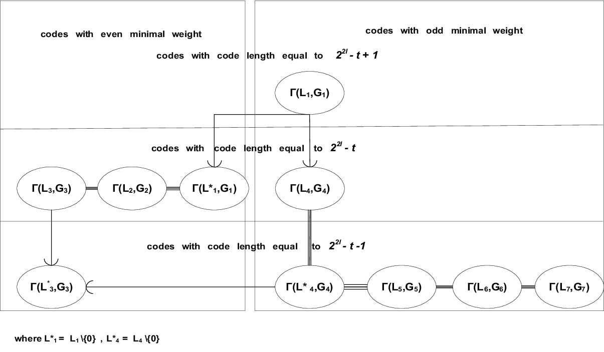
Refer to caption
Fig. 1: Code chain
Definition 3

Let us define a subcode Γ⁡(L3∗,G3)\Gamma(L_{3}^{\ast},G_{3}) of the code Γ⁡(L3,G3)\Gamma(L_{3},G_{3}) as shortened by a position corresponding to the element 00 from L3={α1,α2,…,αn3−1,0}L_{3}=\{\alpha_{1},\alpha_{2},...,\alpha_{n_{3}-1},0\}. Hence Γ⁡(L3∗,G3)⊂Γ⁡(L3,G3)\Gamma(L_{3}^{\ast},G_{3})\subset\Gamma(L_{3},G_{3}) and n3∗=n3−1n_{3}^{\ast}=n_{3}-1 , k3∗=k3−1k_{3}^{\ast}=k_{3}-1 and L3∗=L3\{0}L_{3}^{\ast}=L_{3}\backslash\{0\} .

Lemma 6

Γ⁡(L3∗,G3)⊂Γ⁡(L4,G4)\Gamma(L_{3}^{\ast},G_{3})\subset\Gamma(L_{4},G_{4}) where G4​(x)=At​xt+At−1​xt−1+1G_{4}(x)=A^{t}x^{t}+A^{t-1}x^{t-1}+1, AA ∈G​F​(22​l)\in GF(2^{2l}).

Proof:

It follows directly from the above presentation of the matrix H3.H_{3}. ∎

Corollary 4

[H1∗11...1]\left[\begin{array}[]{c}H_{1}^{\ast}\\ \begin{array}[]{cccc}1&1&...&1\end{array}\end{array}\right]= [H4∗01​…​11].\left[\begin{array}[]{cc}H_{4}^{\ast}&0\\ 1...1&1\end{array}\right].

Proof:

It follows directly from Lemma 3 where we have proved the equivalence of two codes: Γ⁡(L2,G2)\Gamma(L_{2},G_{2}) andΓ⁡(L3,G3)\ \Gamma(L_{3},G_{3}) . ∎

Lemma 7

Γ⁡(L4,G4)≡Γ⁡(L5,G5)\Gamma(L_{4},G_{4})\equiv\Gamma(L_{5},G_{5}) where G5​(x)=C​xt+1+At​xt+A​xG_{5}(x)=Cx^{t+1}+A^{t}x^{t}+Ax,C∈G​F​(2l),\ C\in GF(2^{l}), and AA ∈G​F​(22​l)\in GF(2^{2l}) .

Proof:

It is easy to show that G5​(x)=x∗G4​(x)G_{5}(x)=x\ast G_{4}(x)\ and L5=L4\{0}L_{5}=L_{4}\backslash\{0\}.

Obviously, by substiting xx to A−1​C​xA^{-1}Cx in G5​(x)G_{5}(x) we obtain the same Γ⁡(L5,G5∗)\Gamma(L_{5},G_{5}^{\ast}) code with a more simple G5∗​(x)=xt+1+xt+x.G_{5}^{\ast}(x)=x^{t+1}+x^{t}+x.

The parity-check matrix for this code is:

H5=[1α1t+1+α1t+α1...1αn5t+1+αn5t+αn5α1α1t+1+α1t+α1...αn5αn5t+1+αn5t+αn5...α1tα1t+1+α1t+α1...αn5tαn4−1t+1+αn4−1t+αn5]=[1α1​(α1t+αt−1+1)...1αn5​(αn5t+αn5t−1+1)1α1t+α1t−1+α1...αn5t+αn5t−1+αn5...α1t−1α1t+α1t−1+α1...αn5t−1αn4−1t+αn4−1t−1+αn5].H_{5}=\left[\begin{array}[]{ccc}\frac{1}{\alpha_{1}^{t+1}+\alpha_{1}^{t}+\alpha_{1}}&...&\frac{1}{\alpha_{n_{5}}^{t+1}+\alpha_{n_{5}}^{t}+\alpha_{n_{5}}}\\ \frac{\alpha_{1}}{\alpha_{1}^{t+1}+\alpha_{1}^{t}+\alpha_{1}}&...&\frac{\alpha_{n_{5}}}{\alpha_{n_{5}}^{t+1}+\alpha_{n_{5}}^{t}+\alpha_{n_{5}}}\\ .&.&.\\ \frac{\alpha_{1}^{t}}{\alpha_{1}^{t+1}+\alpha_{1}^{t}+\alpha_{1}}&...&\frac{\alpha_{n_{5}}^{t}}{\alpha_{n_{4}-1}^{t+1}+\alpha_{n_{4}-1}^{t}+\alpha_{n_{5}}}\end{array}\right]=\left[\begin{array}[]{ccc}\frac{1}{\alpha_{1}(\alpha_{1}^{t}+\alpha^{t-1}+1)}&...&\frac{1}{\alpha_{n_{5}}(\alpha_{n_{5}}^{t}+\alpha_{n_{5}}^{t-1}+1)}\\ \frac{1}{\alpha_{1}^{t}+\alpha_{1}^{t-1}+\alpha_{1}}&...&\frac{{}}{\alpha_{n_{5}}^{t}+\alpha_{n_{5}}^{t-1}+\alpha_{n_{5}}}\\ .&.&.\\ \frac{\alpha_{1}^{t-1}}{\alpha_{1}^{t}+\alpha_{1}^{t-1}+\alpha_{1}}&...&\frac{\alpha_{n_{5}}^{t-1}}{\alpha_{n_{4}-1}^{t}+\alpha_{n_{4}-1}^{t-1}+\alpha_{n_{5}}}\end{array}\right].

Therefore H5=H4∗H_{5}=H_{4}^{\ast} according to Corollary 2 . ∎

Lemma 8

Γ⁡(L5,G5)≡Γ⁡(L6,G6)\Gamma(L_{5},G_{5})\equiv\Gamma(L_{6},G_{6}) where G6​(x)=R​xt+1+Vt​xt+V​x+1G_{6}(x)=Rx^{t+1}+V^{t}x^{t}+Vx+1, R∈G​F​(2l),R\in GF(2^{l}), and VV ∈G​F​(22​l)\in GF(2^{2l}) .

Proof:

Using the x+βx+\beta substitution for a variable xx we obtain:

G5​(x+β)=G_{5}(x+\beta)= C​xt+1+(At+C​β)​xt+(A+C​βt)​x+(C​βt+1+At​βt+A​β)Cx^{t+1}+(A^{t}+C\beta)x^{t}+(A+C\beta^{t})x+(C\beta^{t+1}+A^{t}\beta^{t}+A\beta)

where β:\beta: β∈G​F​(22​l)\beta\in GF(2^{2l}) and β≠AtC\beta\neq\frac{A^{t}}{C}. Notice that (A+C​βt)=(At+C​β)t(A+C\beta^{t})=(A^{t}+C\beta)^{t} and

(C​βt+1+At​βt+A​β)t=C​βt+1+A​β+At​βt(C\beta^{t+1}+A^{t}\beta^{t}+A\beta)^{t}=C\beta^{t+1}+A\beta+A^{t}\beta^{t}.

Therefore (C​βt+1+At​βt+A​β)∈G​F​(2l).(C\beta^{t+1}+A^{t}\beta^{t}+A\beta)\in GF(2^{l}).

G6​(x)=1C​βt+1+At​βt+A​β​G5​(x+β)=C(C​βt+1+At​βt+A​β)​xt+1+(At+C​β)(C​βt+1+At​βt+A​β)​xt+(A+C​βt)(C​βt+1+At​βt+A​β)​x+1,G_{6}(x)=\frac{1}{C\beta^{t+1}+A^{t}\beta^{t}+A\beta}G_{5}(x+\beta)=\frac{C}{(C\beta^{t+1}+A^{t}\beta^{t}+A\beta)}x^{t+1}+\frac{(A^{t}+C\beta)}{(C\beta^{t+1}+A^{t}\beta^{t}+A\beta)}x^{t}+\frac{(A+C\beta^{t})}{(C\beta^{t+1}+A^{t}\beta^{t}+A\beta)}x+1,

G6​(x)=R​xt+1+Vt​xt+V​x+1G_{6}(x)=Rx^{t+1}+V^{t}x^{t}+Vx+1

where R=C(C​βt+1+At​βt+A​β)R=\frac{C}{(C\beta^{t+1}+A^{t}\beta^{t}+A\beta)} and V=(A+C​βt)(C​βt+1+At​βt+A​β)V=\frac{(A+C\beta^{t})}{(C\beta^{t+1}+A^{t}\beta^{t}+A\beta)}.

This means that Γ⁡(L5,G5)≡Γ⁡(L6,G6)\Gamma(L_{5},G_{5})\equiv\Gamma(L_{6},G_{6}). ∎

Lemma 9

Γ⁡(L6,G6)≡Γ⁡(L7,G7)\Gamma(L_{6},G_{6})\equiv\Gamma(L_{7},G_{7}) where G7​(x)=B​xt+1+1G_{7}(x)=Bx^{t+1}+1, B=α2l−1,B=\alpha^{2^{l}-1}, and α\alpha is a primitive element of G​F​(22​l)GF(2^{2l}).

Proof:

It can be proved in the same way as the previous Lemma by using the x+βx+\beta substitution for a variable xx where β=VtR\beta=\frac{V^{t}}{R} . ∎

In Figure 1 we present the structure of the code chain. It is possible to define the similar code chain for the codes described in paper [15].

III Minimal distance of subfield subcodes

Lemma 10

The minimal distance of the last Goppa code in the chain Γ⁡(L7,G7)\Gamma(L_{7},G_{7}) exactly equals to its design distance, i.e. d=2​(t+1)+1d=2(t+1)+1.

Proof:

It is easy to show that a polynomial x2l+1−1\ x^{2^{l}+1}-1 can be presented as a product ∏i=12l+1(x−αi⁡(2l−1))\prod\limits_{i=1}^{2^{l}+1}(x-\alpha^{i(2^{l}-1)}) where α\alpha is a primitve element of G​F​(22​l)GF(2^{2l}). Choose some element AA from G​F​(22​l)GF(2^{2l}) such that A2l+1A^{2^{l}+1} ≠1\neq 1 and let B=A−1.B=A^{-1}. Thus we can calculate two polynomials with all different roots {A​αi⁡(2l−1)}\{A\alpha^{i(2^{l}-1)}\} and {B​αi⁡(2l−1)}\{B\alpha^{i(2^{l}-1)}\} i=1,..,2l+1.i=1,..,2^{l}+1.

x2l+1−A2l+1=∏i=12l+1(x−A​αi⁡(2l−1)),x^{2^{l}+1}-A^{2^{l}+1}=\prod\limits_{i=1}^{2^{l}+1}(x-A\alpha^{i(2^{l}-1)}),

x2l+1−B2l+1=∏i=12l+1(x−B​αi⁡(2l−1))x^{2^{l}+1}-B^{2^{l}+1}=\prod\limits_{i=1}^{2^{l}+1}(x-B\alpha^{i(2^{l}-1)}).

The result of the multiplication of these two polynomials and xx :

x⁡(x2l+1−A2l+1)​(x2l+1−B2l+1)=x2l+1+3−(A2l+1+B2l+1)​x2l+2−xx(x^{2^{l}+1}-A^{2^{l}+1})(x^{2^{l}+1}-B^{2^{l}+1})=x^{2^{l+1}+3}-(A^{2^{l}+1}+B^{2^{l}+1})x^{2^{l}+2}-x.

A formal derivative of result of this multiplication:

x2l+1+2−1x^{2^{l+1}+2}-1.

Now consider a binary vector a=(a0​a1​…​an)a=(a_{0}a_{1}...a_{n}) with nonzero elements on and only on positions βj\beta_{j}, (j=1,..,(2l+1+3))(j=1,..,(2^{l+1}+3)) from the following subset of LL:

{{Aαi⁡(2l−1)},i=1,..,2l+1}∪{{Bαi⁡(2l−1)},i=1,..,2l+1}∪{0}\{\{A\alpha^{i(2^{l}-1)}\},i=1,..,2^{l}+1\}\cup\{\{B\alpha^{i(2^{l}-1)}\},i=1,..,2^{l}+1\}\cup\{0\} .

From the definition of the Goppa code, this vector will be a codeword of Γ⁡(L7,G7):\Gamma(L_{7},G_{7})\ :

∑j=12l+1+3ai​1x−βj≡x2l+1+2−1x2l+1+3−(A2l+1+B2l+1)​x2l+2−x≡0​m​o​d​x2l+1−1\sum\limits_{j=1}^{2^{l+1}+3}a_{i}\frac{1}{x-\beta_{j}}\equiv\frac{x^{2^{l+1}+2}-1}{x^{2^{l+1}+3}-(A^{2^{l}+1}+B^{2^{l}+1})x^{2^{l}+2}-x}\equiv 0modx^{2^{l}+1}-1

where βj∈{{Aαi⁡(2l−1)},i=1,..,2l+1}∪{{Bαi⁡(2l−1)},i=1,..,2l+1}∪{0}\beta_{j}\in\{\{A\alpha^{i(2^{l}-1)}\},i=1,..,2^{l}+1\}\cup\{\{B\alpha^{i(2^{l}-1)}\},i=1,..,2^{l}+1\}\cup\{0\}.

Therefore the minimal distance of the Goppa code Γ⁡(L7,G7)\Gamma(L_{7},G_{7}) is equal to the design distance 2l+1+32^{l+1}+3. ∎

Corollary 5

The minimal distance of the equivalent Goppa codes Γ⁡(L6,G6)\Gamma(L_{6},G_{6}) and Γ⁡(L5,G5)\Gamma(L_{5},G_{5}) is exactly equal to its design distance, i.e. d=2​(t+1)+1d=2(t+1)+1.

IV Minimal distance of quadratic trace subcodes

Lemma 11

The minimal distance of the equivalent Goppa codes Γ⁡(L2,G2)\Gamma(L_{2},G_{2}) and Γ⁡(L3,G3)\Gamma(L_{3},G_{3}) is exactly equal to the minimal even weight of a codeword of the code Γ⁡(L5,G5)≡Γ⁡(L6,G6)≡Γ⁡(L7,G7)\Gamma(L_{5},G_{5})\equiv\Gamma(L_{6},G_{6})\equiv\Gamma(L_{7},G_{7}) , i.e. d≥2​(t+1)+2d\geq 2(t+1)+2.

Proof:

It follows directly from the parity check matrixes H3,H2H_{3},H_{2} and H5H_{5}. ∎

It is necessary to note that P.Veron in [13] has proved that the Hamming weight of all codewords of these codes is even.

V Minimal distance of the new code

Lemma 12

The minimal distance of the Γ⁡(L4,G4)\Gamma(L_{4},G_{4}) and Γ⁡(L4∗,G4)\Gamma(L_{4}^{\ast},G_{4}) Goppa codes is exactly equal to its design distance, i.e. d=2​(t+1)+1d=2(t+1)+1 .

Proof:

It follows directly from the equivalence of codes Γ⁡(L4,G4)\Gamma(L_{4},G_{4}) and Γ⁡(L5,G5)\Gamma(L_{5},G_{5}) (Lemma 7). ∎

VI Conclusion

Parameters of the codes forming a chain are presented in Table 1.

Table 1 Parameters of the code chain

Γ\Gamma(L, G)-code with
parity check matrix
code length
number of
information symbols
minimal distance
Γ⁡(L1,G1)\Gamma(L_{1},G_{1}), where
G1​(x)=xt−1+1G_{1}(x)=x^{t-1}+1
parity check matrix: H1H_{1}
n1=22​l−t+1n_{1}=2^{2l}-t+1 k1=22​l−t−2​l​(t−32)k_{1}=2^{2l}-t-2l(t-\frac{3}{2})[9] d1=2​t−1d_{1}=2t-1[7]
Γ⁡(L1∗,G1)\Gamma(L_{1}^{\ast},G_{1}) , where
G1​(x)=xt−1+1G_{1}(x)=x^{t-1}+1 , L1∗=L1\{0}L_{1}^{\ast}=L_{1}\backslash\{0\}
parity check matrix: [H1∗1​…​1]\left[\begin{array}[]{c}H_{1}^{\ast}\\ 1...1\end{array}\right]
n1∗=22​l−tn_{1}^{\ast}=2^{2l}-t k1∗=k1−1k_{1}^{\ast}=k_{1}-1
d1∗d_{1}^{\ast} is even
and equals to
the minimal
even weight
of a codeword
from the code
Γ⁡(L1,G1)\Gamma(L_{1},G_{1})
Γ⁡(L2,G2)\Gamma(L_{2},G_{2}), where
G2​(x)=At​xt+A​xG_{2}(x)=A^{t}x^{t}+Ax
parity check matrix: [H1∗1​…​1]\left[\begin{array}[]{c}H_{1}^{\ast}\\ 1...1\end{array}\right]
n2=22​l−tn_{2}=2^{2l}-t
k2=k1−1k_{2}=k_{1}-1 (Lemma 2)
k2=22​l−t−2​l​(t−32)−1k_{2}=2^{2l}-t-2l(t-\frac{3}{2})-1[8]
d2=d1∗d_{2}=d_{1}^{\ast}
Γ⁡(L3,G3)\Gamma(L_{3},G_{3}), where
G3​(x)=At​xt+A​x+CG_{3}(x)=A^{t}x^{t}+Ax+C
parity check matrix:[H4∗01​…​11]\left[\begin{array}[]{cc}H_{4}^{\ast}&0\\ 1...1&1\end{array}\right]
n3=22​l−tn_{3}=2^{2l}-t k3=k2k_{3}=k_{2} (Lemma 3) d3=d1∗d_{3}=d_{1}^{\ast}
Γ⁡(L3∗,G3)\Gamma(L_{3}^{\ast},G_{3}), where
G3​(x)=At​xt+A​x+CG_{3}(x)=A^{t}x^{t}+Ax+C , L3∗=L3\{0}L_{3}^{\ast}=L_{3}\backslash\{0\}
parity check matrix:[H4∗1​…​1]\left[\begin{array}[]{c}H_{4}^{\ast}\\ 1...1\end{array}\right]
n3∗=22​l−t−1n_{3}^{\ast}=2^{2l}-t-1 k3∗=k3−1k_{3}^{\ast}=k_{3}-1 (Definition 2) d3=d1∗d_{3}=d_{1}^{\ast}
Γ⁡(L4,G4)\Gamma(L_{4},G_{4}), where
G4​(x)=At​xt+At−1​xt−1+1G_{4}(x)=A^{t}x^{t}+A^{t-1}x^{t-1}+1
parity check matrix: H4∗H_{4}^{\ast}
n4=22​l−tn_{4}=2^{2l}-t k4=k4∗k_{4}=k_{4}^{\ast} (Corollary 2) d4=d7d_{4}=d_{7}
Γ⁡(L4∗,G4)\Gamma(L_{4}^{\ast},G_{4}) , where
G4​(x)=At​xt+At−1​xt−1+1G_{4}(x)=A^{t}x^{t}+A^{t-1}x^{t-1}+1 , L4∗=L4\{0}L_{4}^{\ast}=L_{4}\backslash\{0\}
parity check matrix: H4∗H_{4}^{\ast}
n4∗=22​l−t−1n_{4}^{\ast}=2^{2l}-t-1 k4∗=k3k_{4}^{\ast}=k_{3} (Lemma 6) d4∗=d7d_{4}^{\ast}=d_{7}
Γ⁡(L5,G5)\Gamma(L_{5},G_{5}), where
G5​(x)=C​xt+1+At​xt+A​xG_{5}(x)=Cx^{t+1}+A^{t}x^{t}+Ax
parity check matrix: H4∗H_{4}^{\ast}
n5=22​l−t−1n_{5}=2^{2l}-t-1 k5=k4k_{5}=k_{4} (Lemma 7) d5=d7d_{5}=d_{7}
Γ⁡(L6,G6)\Gamma(L_{6},G_{6}), where
G6​(x)=R​xt+1+Vt​xt+V​x+1G_{6}(x)=Rx^{t+1}+V^{t}x^{t}+Vx+1
parity check matrix: H4∗H_{4}^{\ast}
n6=22​l−t−1n_{6}=2^{2l}-t-1 k6=k4k_{6}=k_{4} (Lemma 8) d6=d7d_{6}=d_{7}
Γ⁡(L7,G7)\Gamma(L_{7},G_{7}), where
G7​(x)=xt+1+1G_{7}(x)=x^{t+1}+1
parity check matrix: H4∗H_{4}^{\ast}
n7=22​l−t−1n_{7}=2^{2l}-t-1
k7=k4k_{7}=k_{4} (Lemma 9)
k7=22​l−t−2​l​(t−32)−1k_{7}=2^{2l}-t-2l(t-\frac{3}{2})-1[9]
d7=2​t+3d_{7}=2t+3
(Lemma 11)

In Table 2 we present the quasi-cyclic Goppa codes from our chain. It is easy to see that by substituting xx by β​x+γ\beta x+\gamma we will obtain the same code if the Goppa polynomial is invariant to this substitution: α​G​(x)=G⁡(β​x+γ)\alpha G(x)=G(\beta x+\gamma) where α,β,γ∈G​F​(22​l)\alpha,\beta,\gamma\in GF(2^{2l}) .

In Table 2 we present such values of γ\gamma and β\beta for the Goppa codes from our chain.

Table 2 Quasi cyclic Goppa codes

code G(x) γ\gamma β\beta
Γ⁡(L1,G1)\Gamma(L_{1},G_{1}) xt−1+1x^{t-1}+1 00 any nonzero element from G​F​(2l)GF(2^{l})
Γ⁡(L2,G2)\Gamma(L_{2},G_{2}) At​xt+A​xA^{t}x^{t}+Ax A−1​o​rA^{-1}or 00 any nonzero element from G​F​(2l)GF(2^{l})
Γ⁡(L3,G3)\Gamma(L_{3},G_{3}) At​xt+A​x+CA^{t}x^{t}+Ax+C γ∈G​F​(22​l):\gamma\in GF(2^{2l}): At​γt+A​γ=C⁡(1+β)A^{t}\gamma^{t}+A\gamma=C(1+\beta) any nonzero element from G​F​(2l)GF(2^{l})
Γ⁡(L5,G5)\Gamma(L_{5},G_{5}) C​xt+1+At​xt+A​xCx^{t+1}+A^{t}x^{t}+Ax γ∈G​F​(22​l):C​γt+1+At​γt+A​γ=0\gamma\in GF(2^{2l}):C\gamma^{t+1}+A^{t}\gamma^{t}+A\gamma=0 β=γ​CAt+1\beta=\frac{\gamma C}{A^{t}}+1
Γ⁡(L7,G7)\Gamma(L_{7},G_{7}) xt+1+1x^{t+1}+1 00 (α2l−1)i\left(\alpha^{2^{l}-1}\right)^{i} ,i=1,…,2l+1,i=1,...,2^{l}+1

α\alpha is a primitive element of G​F​(22​l)GF(2^{2l}) and A∈G​F​(22​l).A\in GF(2^{2l}).

Therefore these quasi-cyclic codes have indexes 2l−12^{l}-1 and 2l+1.2^{l}+1.

References

  • [1] V. D. Goppa, A new class of linear error correcting codes. Probl. Inform.Transm, Vol. 6, No. 3 , pp. 24-30,1970
  • [2] M.Loeloeian and J.Conan, A (55,16,19) binary Goppa code IEEE Trans. on Information Theory, vol. 30, p.773, 1984.
  • [3] S. V. Bezzateev, E. T. Mironchikov and N. A. Shekhunova, One subclass of binary Goppa codes, Proc. XI Simp. Po Probl. Izbit. v Inform. Syst. pp. 140-141, 1986.
  • [4] S.V.Bezzateev and N.A.Shekhunova , On the designed distance of the best known (55,16,19) Goppa code , Probl.Inform.Transm., vol. 23, No 4, p.352, 1987.
  • [5] M.Loeloeian and J.Conan , A transform approach in Goppa codes, IEEE Trans. on Information Theory, vol. 35, pp.105-115, 1987.
  • [6] A.M.Roseiro, J.I.Hall, J.E.Adney and M.Siegel, The trace operator and redundancy of Goppa codes, IEEE Trans. on Information Theory, vol. 38,No.3, pp. 1130-1133, 1992.
  • [7] S.Bezzateev and N. Shekhunova , Subclass of binary Goppa codes with minimal distance equal to the design distance, IEEE Trans. on Information Theory, vol. 41, pp. 554-555, 1995.
  • [8] P. Veron, True dimension of some binary quadratic trace Goppa codes, Designs, Codes and Cryptography, 24, pp. 81-97, 2001.
  • [9] P. Veron, Proof of conjectures on the true dimension of some binary Goppa codes, Designs, Codes and Cryptography, 36, pp.317-325, 2005.
  • [10] N.A.Shekhunova, S.V.Bezzateev and E.T.Mironchikov, A subclass of binary Goppa codes, Probl.Inform.Transm., vol.25, no.3, pp.98-102, 1989.
  • [11] S.V.Bezzateev and N.A.Shekhunova, Quasi-cyclic Goppa codes, IEEE International Symposium on Information Theory, Canada, p.499, 1995.
  • [12] G. Bommer and F. Blanchet, Binary quasicyclic Goppa codes, Designs, Codes and Cryptography, 20, pp.107-124,2000.
  • [13] P. Veron, Goppa codes and trace operator, IEEE Trans. on Information Theory, vol. 44,No.1, pp. 290-295, 1998.
  • [14] G. Maatouk, A.Shokrollahi and M.Cheraghchi,Good Ensembles of Goppa Codes, Ecole Polytachnique Federale De Lausanne,ALGO Lab, , 2007, www. algo.epfl.ch/contents/output/sempr/Ghid_MAATOUK.pdf
  • [15] S.V.Bezzateev and N.A.Shekhunova , A subclass of binary Goppa codes with improved estimation of the code dimension, Designs, Codes and Cryptography, 14, pp.23-38, 1998